

Sub-hourly forecasting of fire potential using machine learning on time series of surface weather variables
Alberto Ardid A * , Andres Valencia A , Anthony Power B , Matthias M. Boer C , Marwan Katurji D , Shana Gross E and David Dempsey AA
B
C
D
E
Abstract
Rapidly developing pre-fire weather conditions contributing to sudden fire outbreaks can have devastating consequences. Accurate short-term forecasting is important for timely evacuations and effective fire suppression measures.
This study aims to introduce a novel machine learning-based approach for forecasting fire potential and to test its performance in the Sunshine Coast region of Queensland, Australia, over a period of 15 years from 2002 to 2017.
By analysing real-time data from local weather stations at a sub-hourly temporal resolution, we aimed to identify distinct weather patterns occurring hours to days before fires. We trained random forest machine learning models to classify pre-fire conditions.
The models achieved high out-of-sample accuracy, with a 47% higher accuracy than the standard fire danger index for the region. When simulating real forecasting conditions, the model anticipated 75% of the fires (11 out of 15).
This method provides objective, quantifiable information, enhancing the precision and effectiveness of fire warning systems.
The proposed forecasting approach supports decision-makers in implementing timely evacuations and effective fire suppression measures, ultimately reducing the impact of fires.
Keywords: early warning, fire danger, fire potential, fire potential forecasting, fire potential probability, machine learning, surface weather variables, time series feature engineering, weather station data.
Introduction
The role of advanced and adaptive fire forecasting systems
Fires play a significant role in terrestrial ecosystems, influencing the carbon cycle and ecological progression through disturbance and regeneration (Bond and Keeley 2005; Scott and Glasspool 2006; Bowman et al. 2009). However, fires can have adverse effects on humans, particularly where wildland and urban environments intersect, leading to significant impacts on infrastructure, ecosystem services, property and human lives (Pettinari and Chuvieco 2020; Burke et al. 2021). The increasing frequency and intensity of fires highlight the need for improved early warning systems. With projected climate shifts (Klausmeyer and Shaw 2009), these systems become crucial for effective fire adaptation and mitigation.
Forecasting the outbreak and spread of fires is inherently complex owing to the interactions of various drivers across diverse spatial and temporal scales, including climate, weather, topography, vegetation and human activity (Archibald et al. 2009). Traditional indices like the Fire Weather Index (FWI; Van Wagner 1974), Fire Behaviour Index (FBI; Hollis et al. 2024) and the Fire Forest Danger Index (FFDI; Griffiths 1999) predict the likelihood and potential danger of fires over different time scales, from daily forecasts to seasonal outlooks. Accurate short-term predictions are essential for immediate resource allocation and emergency response (Abt et al. 2009).
However, many existing systems are not designed for rapidly changing environmental conditions (Sharples et al. 2009; Fox-Hughes 2015). Their primary limitations include unreliability and lack of validation across different contexts. These indices often struggle with diverse geographic conditions, are sensitive to meteorological inputs and time scales (Brody-Heine et al. 2023), and fail to handle rapidly changing scenarios, leading to inaccurate forecasts (Stocks et al. 1989; Gong et al. 2023). Additionally, the static nature of these indices does not accommodate the dynamic changes in fire drivers, which can vary significantly over short periods.
These limitations underscore the need for time-scale-agnostic models that provide continuous monitoring rather than one-off forecasts. Such systems could lead to more adaptive and reliable fire danger forecasting by continuously integrating new data and adjusting to changing conditions, such as shifts in weather patterns, vegetation growth and human activity (Canadell et al. 2021).
Integrating comprehensive fire drivers into modern fire danger assessments
Fire danger assessments now incorporate vegetation, weather, topography and ignition sources (Beverly et al. 2010; Müller et al. 2020; Kaur 2023; Wang et al. 2023), leading to diverse research on fire susceptibility using expertise-based assessments, statistical methods and machine learning (ML) models (Hong et al. 2018; Leuenberger et al. 2018; Zheng et al. 2020). ML models handle large datasets and uncover complex patterns but require extensive data and can lack transparency. Empirical models are easier to interpret but may not capture physical processes accurately. Physics-based models provide detailed simulations but are computationally intensive and require precise input data. Combining these approaches could enhance model accuracy and informativeness.
Physics-based models provide valuable insights into physical phenomena, whereas data-driven ML models are particularly strong in predictive tasks (Jung et al. 2013; Leuenberger et al. 2018; Zhang et al. 2019, 2021; Huot et al. 2020; Bergado et al. 2021; Bjånes et al. 2021; Le et al. 2021; Kondylatos et al. 2022). With their capacity to process complex datasets and model intricate variable relationships, ML models are well suited for producing fine-scale predictions and adapting to new data in real time. Although full-physics models offer detailed representations, they can be computationally intensive, which can limit real-time processing capabilities in certain contexts. In contrast, simpler surrogate or ML models can produce faster inferences, capturing nuanced, dynamic patterns and enhancing forecast reliability through continuous learning and adaptation.
ML models for short-term fire danger provide monthly, weekly (Bjånes et al. 2021; Le et al. 2021; Zhang et al. 2021) and daily (Huot et al. 2020; Bergado et al. 2021; Kondylatos et al. 2022) forecasts. Fires are influenced by complex, rapidly changing weather patterns. Forecasting models that assimilate continuous data and provide frequent updates have an advantage. Existing ML techniques often rely on static data, so there is a need for models that adapt swiftly to changing conditions to reduce prediction uncertainty, especially in regions with variable weather patterns (e.g. Australian bushfire-prone areas; Bell 2019).
Machine learning framework for short-term fire potential forecasting
In this study, we introduce a ML framework for the forecasting of sub-hourly changes in fire potential that incorporates the extraction of precursor drivers and patterns as detectable changes or anomalies in environmental conditions that precede a fire – from a single weather station’s time series, employing time series feature engineering (Christ et al. 2018). This method, originally developed for volcano eruption forecasting (Dempsey et al. 2020), has been adapted for the fire potential forecasting problem. It involves the development of a classification model to estimate the likelihood of a fire occurring, assuming an ignition event takes place. The model looks for weather conditions that have historically allowed fires to ignite and spread. Whereas typical fire danger metrics indicate potential levels of fire intensity, rate of spread, or overall fire behaviour, our models specifically classify the conditions under which fire ignition occurs more frequently. They also calculate the probability of fire in a future window, usually several days, updated at the frequency of the data resolution, which for this study is every 30 min. While still in the prototype phase, our model identified pre-fire conditions and provided advanced warnings for previously unanticipated fire events. During pseudo prospective testing on one station in the Sunshine Coast (Queensland, Australia), it achieved this for 11 out of 15 recent significant fire events, outperforming standard metrics.
In this study, we distinguish between two important concepts: ‘fire danger’ and ‘fire potential’. Fire danger typically refers to an assessment of the fire environment, combining elements such as weather, fuels and topography to estimate the ease of ignition, potential spread rate, difficulty of control and likely impact of fires. Commonly expressed through indices like the Fire Danger Index (FDI), fire danger ratings support fire management strategies and public warnings. Conversely, ‘fire potential’ in this study specifically denotes the likelihood or probability of fire occurrence under certain environmental conditions, assuming an ignition source is present. Rather than evaluating potential fire behaviour, our fire potential focuses on identifying patterns in weather (and, ideally, fuel conditions, though the latter are not considered in this study) historically associated with fire likelihood, enabling real-time updates to anticipate conditions conducive to fire ignition and spread. This differentiation between fire danger and fire potential is important to developing adaptive forecasting systems that respond dynamically to changing conditions.
Methods
We used 30-min observations from a weather station at Sunshine Coast Airport, Australia (Automatic Weather Station (AWS) no. 40861), to develop our fire potential assessment model. This station represents the Sunshine Coast region and provides records from 15 major fires that collectively burned 1304 ha, including a significant fire on 19 January 2017 that burned over 843 ha (64.6% of the total burned area; Supplementary Table S1). This section provides an overview of our methodology; further details on data processing, feature selection, model training and evaluation are provided in the subsequent sub-sections.
The model predicts fire potential by assessing the likelihood of conditions that could support fire spread over the upcoming days, using real-time weather data. Although it does not directly predict ignition, it evaluates factors that influence fire occurrence. The model processes data streams such as air temperature, relative humidity and wind speed (Fig. 1a). For each data stream, we calculate over 700 time series features within 2, 5 and 10-day windows (Fig. 1a), with the maximum forecast window being 10 days. These features serve as predictor variables, which are ranked by statistical significance through a feature selection process. The selected features are then used as inputs to each decision tree within the Random Forest model. Each data point in the pre-fire window (2, 5, or 10 days before a fire) is labelled as either fire or non-fire, creating a binary response variable indicating fire occurrence (Fig. 1b). This response variable guides the model in differentiating between favourable and non-favourable conditions. However, the model’s predictability may be limited by rapid, short-term weather fluctuations that are not fully captured within these forecast windows, especially when fire conditions change abruptly.
Methodology workflow. (a) Data pre-processing: collect data streams (temperature, relative humidity, wind speed) and calculate time series features. For each data stream in each window, we calculate over 700 time series features (e.g. mean, s.d., number of peaks, Fourier coefficients, entropy, quantiles). (b) Model training and testing: construct a label vector by assigning binary labels (1 for pre-fire data, 0 for non-fire data) based on pre-fire windows of 2, 5, or 10 days. Train multiple decision trees using these features and label vectors, averaging their outputs to form a random forest model. The model’s output, called ‘consensus,’ ranges from 0 to 1. Test the model using leave-one-out cross-validation, where each fire episode (defined as the 8-week period centred on the reported fire date) is excluded once for validation. Aggregate model performance to compute true and false positive rates for all thresholds and plot these in a receiver operator characteristic (ROC) curve. (c) Implementation and early warning: use the trained model to assimilate real-time weather data, running in the cloud or on a local PC, providing a consensus value for each input set, updating every 30 min. Downloading new data, running the trained model and computing the output takes minutes. Based on historical model performance and the current state, compute risk metrics such as the conditional probability of a fire and the hazard ratio, which measures the relative probability of having a fire compared with not having a fire in the next 10 days.
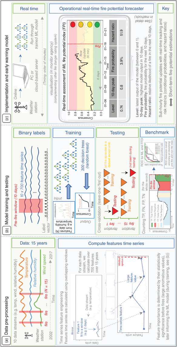
Three separate models were trained on historical weather data to evaluate how far in advance they could identify weather sequences or features indicative of favourable conditions for fire starts. The Random Forest model outputs a consensus value between 0 and 1, reflecting the similarity between current data and pre-fire conditions. This consensus score is derived from the relative frequency of feature usage across all decision trees, though it does not assign specific weights to predictors in the traditional sense. The model updates predictions every 30 min with real-time data to continuously assess fire potential (Fig. 1c). Each 30-min update incorporates information from the past 2, 5 and 10 days, with the 10-day window representing the maximum period of data considered for assessing current conditions, rather than producing a forecast that extends 10 days into the future. In pseudo-prospective forecasting, forecasts are constructed for data withheld during model training (out-of-sample testing). This approach approximates, but does not perfectly replicate, prospective forecasting conditions, providing a better performance assessment than a hindcast. For test data, feature time series are calculated using overlapping windows that advance by 30 min. This set-up mimics real-time fire monitoring. Features from each subsequent window are passed to the trained Random Forest model. The binary outputs of each decision tree are averaged to produce a consensus value ranging from 0 to 1, with values closer to 1 representing higher consensus.
Forecast evaluation aims to determine overall accuracy, including false positive and false negative rates, and the correlation between forecast probabilities and actual outcomes over long periods. Accuracy can be evaluated in both pseudo-prospective and prospective scenarios, with the latter requiring real-time or future data to assess a frozen model. Although pseudo-prospective forecast performance may not perfectly mirror real-time prospective performance, it provides a better assessment than a hindcast.
Data processing
The weather time series spans 15.4 years (1 March 2002 to 31 July 2017) at half-hourly frequency, covering 15 significant fires (Supplementary Table S1). Each weather time series, referred to as a data stream (Fig. 1a), includes variables such as air temperature (T), dew point (DP), relative humidity (RH), wind speed (V), potential air temperature (Theta), Keetch–Byram Drought Index (KBDI), drought factor (DF), saturated vapour pressure (SVP), actual vapour pressure (AVP), vapour pressure deficit (VPD), Fine Fuel Moisture Code (FFMC) and Grass FFMC. These variables indicate fuel dryness and fire weather conditions, relevant for anticipating the likelihood of ignition and subsequent fire spread and behaviour.
For forests and woodlands, these variables are appropriate as they account for conditions influencing fire ignition and spread. In grass-dominated, arid environments, additional predictors such as preceding months of grass growth detected by NDVI (Normalized Difference Vegetation Index), grass curing percentage, or other spectral vegetation indices should ideally be included to reflect different environmental factors influencing fire activity. However, these additional parameters are not used in the current study, as our focus is specifically on fire-prone conditions in forested and woodland areas.
This analysis seeks to identify changes in fire weather that impact fire potential, providing insights for responsive fire management measures. Data time series were divided into 2, 5 and 10-day windows to capture varying temporal patterns indicative of fire potential. The choice of these windows reflects different weather influences on fire risk: the 2-day window captures short-term diurnal variations, which are generally reliable for stable conditions, the 5-day window captures medium-term fluctuations and the 10-day window identifies broader weather trends. This range helps in detecting both rapid and gradual changes in conditions conducive to fire outbreaks. These windows were chosen to account for the cumulative effects of weather patterns on fire-prone conditions rather than immediate, isolated forecasts.
Within each window, over 700 features are calculated using the Python package ‘tsfresh’ (Christ et al. 2018). These features include several key families that contribute to the model’s predictive capability. Statistical measures, such as mean and standard deviation, summarise the overall level and variability of essential weather variables like air temperature, humidity and wind speed. For instance, high mean air temperatures or low relative humidity values can increase likelihood of fire by creating drier fuel conditions, whereas high variability may indicate unstable conditions conducive to fire spread. Frequency-domain features, such as Fourier coefficients, capture periodic patterns in the data, enabling the model to detect cyclical changes, such as daily temperature or humidity cycles. Recognising these cycles is important, as shifts in regular weather patterns – such as prolonged heat during the day – can signal increased fire potential. Data distribution measures, including quantiles and the number of peaks, help identify extreme values and distributional shifts in weather data, highlighting high-risk periods. For example, high quantiles of wind speed may indicate gusty conditions that could accelerate fire spread, whereas low quantiles of humidity might signal particularly dry conditions. Lastly, non-linearity and complexity measures, like entropy, quantify irregular or complex patterns in the data, potentially revealing unpredictable or chaotic weather changes that often correlate with fire-prone conditions. Together, these diverse feature types enable the model to identify subtle and complex precursors to fire potential across multiple timescales.
To prevent data leakage, features are computed based on data up to the current timestamp within each window, a method referred to as ‘looking back’. Mathematically, this means each feature is calculated only using data from times t – w to t, where w is the window length. This backward-only approach ensures that no future information is included in feature calculations, simulating real-time forecasting conditions.
Model training and testing
We define a classification problem that focuses on detecting signals within pre-fire windows (2, 5, or 10 days before fires). Data points within these pre-fire windows are labelled ‘1’ (indicating fire-prone conditions), while all other points are labelled ‘0’ (non-fire conditions). For example, using a 2-day pre-fire window with 75% overlap results in approximately 60 label-1 windows, compared with over 15,000 label-0 windows. This disparity illustrates the class imbalance, where non-fire instances far outnumber pre-fire instances. To address this, later we employ random under-sampling of label-0 windows to achieve a balanced dataset, repeating the sampling process multiple times to mitigate the effects of randomness. This approach ensures that the model learns to distinguish between pre-fire and non-fire conditions effectively, enhancing its predictive accuracy and robustness.
Features are ranked by statistical significance using the Mann–Whitney U test (McKnight and Najab 2010), retaining those with P values below an adjusted Benjamini–Yekutieli threshold (Benjamini and Yekutieli 2001). The top-ranked features are then used to train a Random Forest model consisting of up to 300 decision trees, each trained on different subsets of down-sampled windows. This method outputs a consensus value between 0 and 1, indicating the similarity between current data and pre-fire conditions. Model training is implemented using the scikit-learn Python library (Pedregosa et al. 2011).
We assess model performance using a leave-one-out cross-validation (LOO-CV) approach, specifically designed to simulate realistic out-of-sample conditions for fire events. In this approach, each fire episode is defined as an 8-week period centred on the fire date. For each fire event, all data from the corresponding 8-week period is withheld from model training and feature selection, treating it as an independent testing set. This process is repeated for each fire event, ensuring that each one is tested as a distinct, out-of-sample test case, while the model is trained on the remaining data – including non-fire periods and data from all other fire events. This set-up allows us to test model performance across all fire events individually, while preserving the independence of each validation period.
To address the natural imbalance between fire and non-fire data, we applied an under-sampling technique to the non-fire periods, creating a balanced training set with an equal representation of fire and non-fire instances. Rather than using a class weight adjustment, we opted for under-sampling, which selectively retains non-fire data across subsets to achieve an approximately 1:1 ratio between fire and non-fire instances – a standard metric for class balance. This balanced representation ensures that the model is not biased toward the more frequent non-fire class and can accurately differentiate between fire-prone and non-fire conditions. Additionally, the under-sampling approach captures the variability of non-fire conditions by maintaining a sparse yet diverse set of instances, which helps the model generalise well across both scenarios. This balance reduces the risk of overfitting to specific non-fire patterns, ultimately enhancing the model’s robustness and predictive accuracy across diverse conditions.
For testing, feature time series are calculated using overlapping windows that advance every 30 min. This set-up mimics real-time fire monitoring, with each new feature window sequentially passed to the trained Random Forest model. The individual decision tree outputs are then averaged to produce a consensus score between 0 and 1, where higher values indicate a stronger similarity to pre-fire conditions. This pseudo-prospective forecasting approach, which withholds certain data entirely from model training to simulate out-of-sample conditions, provides a more realistic performance assessment than traditional hindcasting, which uses historical data inclusively and may overlap with training data (Ardid et al. 2023). By approximating real-time forecasting conditions, pseudo-prospective forecasting offers a closer evaluation of model performance in operational settings.
ROC curves evaluate the model’s ability to classify pre-fire and non-fire data. These curves plot the true positive rate (sensitivity) against the false positive rate (1 – specificity) across various thresholds. Models are computed across 100 thresholds from 0 to 1, with the area under the ROC curve (AUC) indicating performance. Steps to construct ROC curves include selecting a threshold, applying it to forecasts, scoring true/false positives and negatives, and calculating true positive rate (TPR) and false positive rate (FPR). This evaluation helps determine the optimal threshold for reliable fire potential forecasting.
For benchmarking, FFDI values are computed at the same frequency as ML models and their ROC curves compared. FFDI forecast consensus is determined by converting FFDI records to percentile values. As with ML models, 100 quantile thresholds are used to compute TPR, FPR and ROC curves, serving as a reference case.
Early warning model
For illustration purposes, we implemented a simple warning model with a 48-h look-forward period. The consensus output, which updates every 30 min, is compared with a predetermined threshold between 0 and 1. If the consensus exceeds this threshold, a fire potential warning is issued for the following 48 h. Each time the consensus score goes above the threshold, the 48-h warning period restarts. The decision to maintain the warning level beyond 48 h is arbitrary at this stage but is based on the rationale that prolonged high consensus scores indicate sustained fire-prone conditions, which should keep the warning active. The warning is rescinded only if the consensus remains at or below the threshold for a consecutive 48-h period. Future implementations of this warning model may adapt the duration and criteria based on specific forecast user needs.
This modified version of the ROC curve is designed for an optimised warning system. It takes into account true positives, false positives, true negatives and false negatives based on the warning model described above. This metric has been explored for volcano eruption forecasting (Dempsey et al. 2022). The warning system becomes active when the forecast model output (y) reaches or exceeds a predetermined trigger threshold (yc). The model is trained to provide a 48-h advance warning, and the warning is cancelled if y falls below yc continuously for 48 h. The parameter yc influences the overall duration of warnings and the number of missed fires (those occurring outside warning periods). By plotting the missed fire rate against the total warning duration for different values of yc, an alternative ROC curve is obtained. This curve helps select an optimal trigger threshold by balancing missed fires (false negatives) and false positives. Different users may choose different thresholds based on their risk tolerance. Therefore, selecting yc involves considering the trade-off between missed fires and false positives, aligning with each user’s specific risk tolerance. Ultimately, the choice depends on the operational requirements and acceptable risk levels of the end user.
For a warning model that has been constructed for M fires, the events are split into subsets of fires occurring inside a warning, Min, and the rest outside, Mout, i.e. Min + Mout = M. The rate of fires when a warning is in effect is:
where τ is the forecast for the look-forward period and Tin is the total length of all warnings. Similarly, the rate of fires outside a warning is:
where Tout is the total length of time not under warning. Assuming a Poisson model of fires, the probability of one or more fires in the forecast period, τ, when a warning is in effect is:
and when a warning is not in effect is:
This assumes that each fire event is independent of others, and the fire rate is constant inside and outside warnings. This necessarily simplified approach is suitable for comparing probabilities in our study. However, more advanced techniques like non-homogeneous Poisson processes could be used to incorporate greater complexity into the probability calculations.
Results
Forecast performance and benchmark
In this research, a good forecasting model is one that outputs a strong positive response (values approaching 1) in the days before a fire and a relatively depressed response (values closer to 0) during the extended periods between fires. The discriminability of these models is quantified by their ROC curve (see Methods) and associated AUC. Discriminability assesses the ability of forecasting models to differentiate between different classes (Ardid et al. 2022), specifically, pre-fire and non-fire data in this context. When discriminability is low, it is probable that forecasts will have unacceptably high rates of false positives.
Fig. 2 provides an overview of the forecast performance of the three models throughout the entire study period, juxtaposed with the reported FFDI values (Fig. 2a). Notably, the values preceding fires from the three models show a distinct separation, or discriminability, from the non-fire data (Fig. 2d, e, f). In contrast, the FFDI values do not display such a clear differentiation (Fig. 2g).
(a–c) The solid lines represent the consensus values of two models, showcasing the output of the trained models over the entire dataset. High values of the models (green and red curves) indicate high fire potential. We test whether the model correctly anticipated fires and examine its values during non-fire periods. The model’s performance over the entire period is evaluated quantitatively later in the histograms (d–g). Additionally, the FFDI values for the entire period are provided. A reference threshold of 0.7 is denoted by a horizontal dashed gray line, while recorded fires in the region are marked by vertical dashed black lines. (d–g) Histograms display the consensus values of three ML models, distinguishing between pre-fire and non-fire values. In panel (f), the same distributions are shown for FFDI values. For these histograms, the greater the separation between the distributions, the more distinct the pre-fire values are from the non-fire values as output by the model and FFDI. This separation is quantified by the Kolmogorov-Smirnov (KS) statistic. A larger split indicates better model performance. Please note that for this histograms, pre-fire values encompass a period of 10 days before the reported fire times, whereas non-fire values cover all days except those within 15 days around the reported fire times.
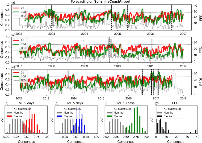
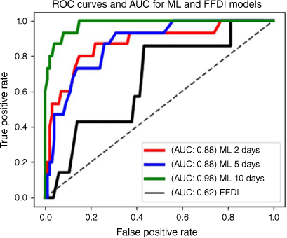
To assess discriminability across various thresholds, we computed ROC curves, which are a graphical measure of the performance of a classification model across all possible thresholds (Fig. 3). As discriminability improves, a ROC curve will depart from the diagonal towards the top left corner, denoting a reduced false positive rate. ROC curves for all forecast models trained on different window size have comparable discriminability, indicating all timescales recover relevant pre-fire patterns information. All models have similar or better discriminability than the existing FFDI (Fig. 3).
ROC curves (receiver operating characteristic) and AUC (area under the curve) illustrating and comparing the performance of three ML forecasting models and a simplified forecaster based on FFDI using thresholds (see Methods). The diagonal line represents a random model (a model that makes predictions with no discrimination between classes), and the AUC in the legends indicates the area under the curve. Each point on the ROC curve corresponds to a threshold (100 evenly spaced thresholds between 0 and 1; see Methods). As the performance of the model improves, the ROC curve departs from the diagonal towards the top left corner, indicating a reduced false positive rate. Using AUC to evaluate performance, we find that ML models improve average performance by 47% compared with the FFDI approach. Among the ML models, the 10-day model outperforms the others regarding discriminability and accuracy.
Although all time windows capture relevant pre-fire patterns, the 10-day window generally performs better than the 2-day window, likely owing to its ability to account for longer-term, cumulative weather conditions that may gradually elevate fire risk. The 2-day window, which focuses on short-term fluctuations, may be more susceptible to rapid weather changes that do not consistently indicate pre-fire conditions, leading to a less stable signal. In some instances, like the fire in 2007 (Fig. 2b), the models trained on different windows may appear anti-correlated. This could be due to short-term weather variations affecting the 2-day model’s predictions while the 10-day model, which averages out short-term noise, maintains a more consistent signal. Thus, the 10-day window may better capture slowly building conditions conducive to fire, providing improved predictive performance in many cases.
Models can be directly compared using the area under the ROC curve (AUC), which is a single numerical measure of average model performance. Using AUC to evaluate performance, we find that ML models improve average performance by 47% over the FFDI approach (Fig. 3).
Interpretability: data streams significance and features that strengthen prior to fires
The combination of time series features engineering with training Random Forest classification models allows us to investigate how the data inform the models. The choice of Random Forest can help to quantify variables’ attribution, interpret models’ predictions and ultimately improve our understanding of the drivers of fires.
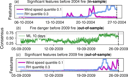
We can identify which data streams and features hold more significance for the accurate forecasting of fire activity. Our ML models exploit this relationship at the time series feature level. For instance, quantile features derived from wind speed and relative humidity data are shown in Fig. 4a before a fire, displaying clear increases and peaks before the event. This and other fires are later used for training a model, where these features were identified as relevant when training the Random Forests among dozens of others. Fig. 4b shows the model output when run over an out-of-sample fire, model that increase before fire, indicating the efficacy of these identified precursors when forecasting an out-of-sample event. This is further emphasised in Fig. 4c, wherein the same features identified as significant when training (Fig. 4a) showed elevated values prior to the 2009 fire.
Illustration of precursor identification and transfer to out-of-sample target fire. The figure demonstrates how significant features identified during model training (in-sample) can be transferred to forecast fire potential in out-of-sample events. The aim here is to show that two features identified during training are triggering the model’s response on out-of-sample data. (a) Wind speed quantile 0.1 (magenta) and relative humidity quantile 0.3 (blue) show elevated levels before the 2004 fire (in-sample). (b) The machine learning model’s fire potential forecast for the 2009 fire (out-of-sample) is shown, with higher consensus values indicating increased fire potential. (c) The same features identified in (a) exhibit elevated levels prior to the 2009 fire (out-of-sample), supporting the transferability of these precursors. Note: the machine learning models developed here exploit learning from weather data at the time series feature level. For example, wind speed quantile 0.1 and relative humidity quantile 0.3 are discriminated in pre-fire sequences from the training ensemble. Later, these same features are seen to strengthen prior to an out-of-sample fire in the target area. This demonstrates the functional basis of precursor transfer among different fire events.
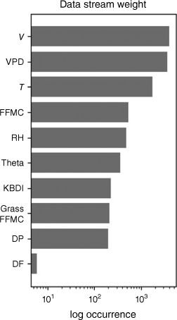
The significance of various data streams within the context of our trained Random Forests provides an extra layer of interpretability, offering insights into the frequency of a data stream’s use in informing decision trees (Fig. 5). Noteworthy trends emerge, with key variables such as temperature (T), RH, wind speed (V), VPD and FFMC being recurrently employed by decision trees. This observation underscores their relevance and role in forecasting fire potential.
Significance of data streams in the trained ML models. This visual depicts the frequency of a data stream’s utilisation in informing all decision trees in the random forest, serving as an indicator of its importance for forecasting fire potential. Higher log occurrences indicate greater importance in the forecasting model. The x-axis represents the log occurrence of each data stream being used in the model’s decision-making process. The data streams include T (temperature), DP (dew point), RH (relative humidity), V (wind speed), Theta (potential temperature), KBDI (Keetch–Byram Drought Index), DF (Drought Factor), VPD (Vapour Pressure Deficit), FFMC (Fine Fuel Moisture Code) and Grass FFMC.
Supporting decisions in warning systems
The objective of natural hazard forecasts is to provide decision-makers with objective, quantitative information regarding the likelihood of an extreme event occurrence within a specified warning period (Sorensen 2000). Here, we consider that warnings could be triggered when the ML model output exceeds a threshold and end once model output has dropped below the threshold for more than 48 h (see Methods).
Fig. 6 shows a modified version of the ROC curve designed specifically for the 10-day optimised warning system that takes into account various metrics such as true positives, false positives, true negatives and false negatives based on a warning window (see Methods). This metric is useful for computing conditional probabilities of having a fire for a certain threshold using historical data and hazard ratios (see Methods). The model applied over the 15.4-year dataset with a threshold of 0.7 accurately forecast 75% of fire potential conditions (11 out of 15; Supplementary Table S1) occurring within the designated warning period, constituting approximately 5% of the total time span, equivalent to 282 days (Fig. 6). This equates to a ~4% probability of fire occurrence in a 48-h period when a warning is in effect, as opposed to a 0.08% chance of a fire during no-warning.
Alternative ROC curve design for an optimised warning system. This figure illustrates the performance of the warning system based on the 10-day ML model tested on the Sunshine Coast record (15.4 years). The ROC curve plots the proportion of fires during alerts (y-axis) against the proportion of days under alert (x-axis) for various threshold values. For a threshold of 0.7 (indicated by the star), the system spends 5.5% of the time under warning, covering 282.6 days, and captures 75.0% of the fires, equating to 11 fires. The calculated rates of fire occurrence are λin = 0.0389 when a warning is in effect and λout = 0.00075 when no warning is active. These translate to probabilities of 3.89 and 0.0749% for fire occurrence in warning and non-warning periods, respectively, yielding a hazard ratio of 51.9. The warning system becomes active when the output of the forecast model reaches or exceeds a predetermined trigger threshold. This system helps to effectively balance the trade-off between missed fires (false negatives) and false alarms (false positives).
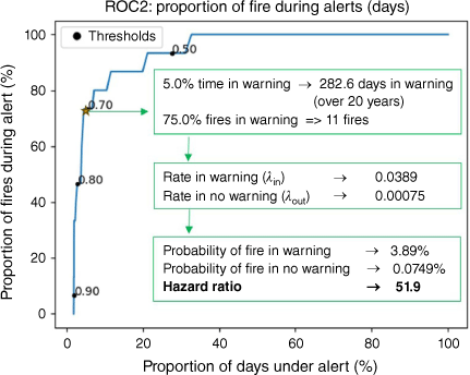
Specifically, the variables indicated in the Methods sections for computing the conditional probabilities and hazard ratio are: Min = 11, Mout = 4, Tin = 282.6 days, Tout = 5369.4 days. The calculated fire rates (per 48 h) are λin = 0.0389 and λout = 0.00075, and the probabilities are Pin = 3.89 and Pout = 0.0749. Finally, the hazard ratio is 51.9 (Fig. 6). Given the inherently low probability of fire events, it is more meaningful to express conditional probabilities as hazard ratios. These ratios quantify forecast accuracy in terms of the relative likelihood of a fire event under different warning conditions. In the example above, fires are predicted to be 50 times more likely during an active warning compared with non-warning conditions.
Discussion
Practical challenges on operational forecasting
Demonstrating the forecasting skill of transferred fire precursors is a necessary but not sufficient step for their operational use. Fire monitoring teams routinely integrate a wide range of signals across disparate time scales (Ghali et al. 2020; Mohapatra and Trinh 2022; Ardid et al. 2024a) and use these to inform mental models (expert judgement) of the evolving fire hazard. If they are to provide complementary input to this process, forecasting models need to be interpretable on a real-time time-series basis. Although this problem remains outstanding, a presentation of individual forecast characteristics is useful here to define its challenging aspects.
A reliable forecast should consistently demonstrate accuracy, free from significant errors or biases, thereby establishing confidence in the forecasting process and its outcomes. In this study, we considered that a fire is anticipated by our forecast fire potential model, i.e. a true positive, if the model output (consensus) surpasses a predetermined threshold the days defined by training window (2, 5, and 10 days) before the recorded fire. Once the model output meets this criterion, it is deemed to have been anticipated. For instance, Fig. 7 shows the out-of-sample performance of the model trained using a 10-day window before the largest fire in our catalogue, which occurred in January 2017. The model’s predictions steadily increase over 2 weeks, reaching a peak a day before the event. The reference threshold is crossed ~4 days before the fire, triggering a warning that continues until the fire occurs. This extended warning period is designed to ensure that high-risk conditions are captured and maintained if fire-prone conditions persist. The warning remains active as long as the model’s output consistently exceeds the threshold, signalling sustained fire potential. If the consensus drops below the threshold for 48 continuous hours, the warning would be cancelled; however, in this instance, conditions remained above the threshold. The FFDI also reaches high values a couple of days before the fire, but its highest values for this period are recorded 2 weeks earlier, over 4 days (7 to 9 January), while the ML model remains low during this period (Fig. 7a). The difference between the consensus model output and FFDI values, despite both using the same weather variables, arises from the time series feature engineering and selection process within our ML approach. This approach allows our model to capture nuanced, longer-term and hidden patterns in the data that may indicate increased fire potential. By identifying these underlying risk factors, our model can provide early indications of fire potential, complementing the FFDI’s real-time responsiveness to immediate conditions.
Performance of the forecasting model trained with a 10-day window prior to the largest fire event in the catalogue, which occurred in January 2017 and burned 843 ha (out-of-sample, i.e. this fire was not considered during training). (a) The model’s consensus output (green line) and FFDI (black line) are plotted against time. The consensus steadily increases over 2 weeks, peaking a day before the fire. The warning threshold (grey dashed line) is crossed approximately 4 days before the fire, triggering a warning period (grey shaded area) that persists until the fire occurs. The fire event is highlighted by a red shaded area. The FFDI also shows increasing values a couple of days before the fire, with the highest values recorded 2 weeks earlier (7 to 9 January), a period during which the ML model remains low. It is important to note that an FFDI of 7 falls into the low/mid category. (b) Time series of wind speed (magenta line), temperature (orange line) and relative humidity (sky blue line) during the same period. The fire event is again highlighted by a red shaded area. This figure illustrates the model’s capability to anticipate fire events by showing a clear increase in the consensus output leading up to the fire, compared with traditional indices like the FFDI.
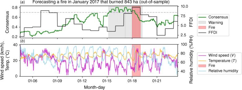
It is notable that the FFDI peaks precisely during the fire event, whereas the event occurs as the consensus from our model begins to decline. This discrepancy may arise from the differences in how FFDI and our model respond to short-term versus accumulated conditions. FFDI is highly sensitive to immediate weather conditions and reflects rapid fluctuations, whereas our model’s consensus score incorporates longer-term fire-prone patterns detected over the prior 10-day period. This approach captures fire risk conditions that build up and signal fire potential in advance rather than aligning with immediate peaks in weather-driven indices. This complementary behaviour between FFDI and our model could provide a large-scale warning system, where early indications from our model can be reinforced by high FFDI values closer to the event, improving operational response.
Across all reported fires, the models exhibit good performance when applied to fires that were not part of the training data, i.e. out-of-sample (Supplementary Figs S1 and S2). Models are effective in forecasting fire potential when there is a significant increase in their output before the fires occur (e.g. Supplementary Fig S1a, d, e, f), but less so when no increase is observed beforehand (Supplementary Fig S1b, c). Nevertheless, the models remain valuable when an elevated value is detected several days before the fires (e.g. Supplementary Fig S1b, c, e, f) as we are estimating fire potential conditions that do not always result in actual fires (see Supplementary Fig S2 for all events). Using a reference threshold of 0.7 (e.g. Fig. 7, Supplementary Fig S1), the highest accuracy achieved by the tested forecasters in predicting out-of-sample fires for the 10-day model was 75% (11 out of 15 fires) (Supplementary Fig S2; Supplementary Table S1). In comparison, the 2 and 5-day models achieved 33 and 20% accuracy, respectively, at this threshold. It is important to note that, by lowering the threshold, it is possible to eventually anticipate all fires. However, it is essential to ensure that the associated false positive rate remains acceptable for the chosen threshold. We explored this balance in previous sections, where we tested a range of thresholds and evaluated different metrics to identify the optimal one (Figs 2, 3).
Assimilating diverse data sources for enhanced fire potential forecasting
Expanding the forecasting framework to include a broader array of time series data, such as remote sensing parameters like drought indices, vegetation health and additional weather variables (Huot et al. 2020), can refine fire potential assessments. Integrating remote sensing data provides a comprehensive environmental view, capturing indicators that may not be discernible through on-site weather station measurements alone. Drought indices reveal soil moisture levels, influencing fuel availability and fire ignition. Vegetation health metrics provide valuable information on landscape flammability, identifying areas prone to rapid fire spread. Including terrain ruggedness is also relevant, as fires in rugged terrain typically escalate owing to topography and the difficulty of early suppression efforts. This diverse data integration allows the model to better understand the complex interplay between environmental conditions and fire behaviour, enhancing accuracy and reliability.
Currently, the model focuses primarily on weather metrics, which does not capture all factors influencing fire behaviour. Understanding the site context is key to evaluating whether weather is the primary driver or if other factors play a significant role, such as fuel properties, fuel connectivity, topographical differences, moisture gradients and atmospheric stability. For example, unanticipated fires might have been influenced by these unaccounted factors. Our data include fires mainly in three areas: Noosa, Mount Coolum and Maroochy River National Parks, each characterised by distinct fuel types – primarily eucalypt, heathland and melaleuca, respectively (Supplementary Table S1). Preliminary analysis suggests that different fuel types may influence fire behaviour and the likelihood of anticipation, with heathland and melaleuca being less likely to be associated with anticipated fires. However, there are not enough data to draw definitive conclusions owing to an unbalanced dataset.
Additionally, live fuel moisture, which refers to the water content in living vegetation, directly impacts flammability and is a significant predictor of fire activity and behaviour (Yebra et al. 2013, 2018). Future work should incorporate complex vegetation and topography (Si et al. 2022), as well as hydrological variables like soil moisture or stream flow data, to improve fire potential forecasts (Farahmand et al. 2020). Factoring in wind direction changes, such as sudden shifts from west to southeast, which are crucial in escalating established fires, could also enhance model precision.
Complementing recent advances in fire danger forecasting
The Australian Fire Danger Rating System (AFDRS) is a new fire danger rating system for Australia calculated daily by the Bureau of Meteorology using forecast weather at hourly intervals on a 1.5 × 1.5 km grid across Australia (Matthews et al. 2019; Hollis et al. 2024). The NSW Rural Fire Service trial of the AFDRS during the 2021–22 bushfire season highlighted the advantages of the new system, despite the need for ongoing adjustments (McCoy and Field 2022). Our study introduces an ML-based framework that uses high-frequency weather data and updates for sub-hourly predictions, improving forecast responsiveness. By leveraging ML models, our framework complements the AFDRS by enhancing the accuracy and timeliness of fire danger forecasts, thus supporting operational responsiveness. This aligns with the goals of the AFDRS to support fire management operations and public communications regarding potential fire danger (Hollis et al. 2024). The modular nature of the AFDRS supports continuous and incremental improvements, incorporating the best available science to estimate fire potential accurately (Hollis et al. 2024). Therefore, our approach could be integrated into the AFDRS framework, allowing improvements in predictive accuracy and operational effectiveness to be evaluated.
Probabilistic forecasting techniques, like those in the Global ECMWF (European Centre for Medium-Range Weather Forecasts) Fire Forecast (GEFF) system (Worsnop et al. 2021), enhance accuracy through statistical post-processing. Our framework aligns with this approach by using ML models to update forecasts in real time. Whereas GEFF focuses on 2-week forecasts for longer-term planning, our model provides immediate, short-term predictions, bridging the gap between long-term and real-time needs. Advancements in deep learning have shown effectiveness in capturing spatio-temporal patterns (Kondylatos et al. 2022). Our framework complements these efforts through time series feature engineering and Random Forest models, which offer some interpretability through feature importance scores. However, the reliance on feature importance from decision trees provides limited insight into causal relationships within the data. To address this, future work could incorporate more advanced interpretability techniques, such as SHAP values (SHapley Additive exPlanations; e.g. Qayyum et al. 2024) or causal inference, to enhance model transparency and improve operational decision-making.
Research in mountainous plateau regions has used logistic regression to address topographical and meteorological complexities (Si et al. 2022). Our framework complements this by capturing fine-scale temporal variations and integrating a broader range of weather variables. However, future work should incorporate complex vegetation and topography to improve precision in challenging environments. The integration of hydrological variables, such as soil moisture, is necessary for enhancing fire danger forecasts (Farahmand et al. 2020). Our current model focuses on weather metrics, but incorporating hydrological data and remote sensing could potentially enhance our predictions. Remote sensing would be particularly beneficial in improving fuels data and accounting for topographic complexity, providing a more comprehensive understanding of the factors influencing fire behaviour.
Multi-station data integration and simplifying the complexity of fire regimes
To improve the accuracy and robustness of fire potential assessments, future work should consider integrating data from multiple stations across diverse eco-regions. This multi-station approach would provide a broader and more comprehensive dataset, allowing the model to capture regional differences in fire occurrence and better adapt to the variability across distinct terrains and ecosystems (Fujioka et al. 2008). Such regional differences are critical, as models developed using data from a single region may not generalise effectively to other eco-regions with unique fire environments – including fire weather, fuels and topography. In areas with complex terrain, individual weather stations may not accurately reflect localised fire–weather interactions. Additionally, fuel type and moisture content are also critical factors influencing ignition and fire spread, further underscoring the importance of a diverse geographic data set.
To simplify the complexity of fire regimes and the diversity of fire-prone ecosystems, we can use the dichotomy between fuel-limited and fuel dryness-limited fire regimes. Fuel-limited fire regimes, found in grass-dominated semiarid interiors, are primarily constrained by the availability of combustible material. In contrast, fuel dryness-limited fire regimes, typical of forests and woodlands with litter fuels, depend on the moisture content of the fuel (Bradstock 2010; Boer et al. 2021). Incorporating these distinctions into the model can help address variability in fire behaviour across ecosystems, considering both weather and fuel conditions for a more comprehensive fire forecasting system. Integrating data from multiple stations across various regions will enhance our understanding by providing diverse observations, refining the model to better capture regional fire behaviour nuances.
Addressing data scarcity challenges through transfer machine learning
In light of the escalating impact of climate change on fires, it is increasingly important to address the issue of data scarcity. For instance, countries with scarce historical data that may be facing increasing fire danger due to a combination of climate conditions, vegetation types and human activities, could benefit from ML models like the one presented here. Our research aims to build models capable of training in one region and applying their forecasting capabilities to another, even in the absence of historical data, by leveraging the principle of transfer ML.
Our approach relies on assimilating 30 min increment time series of weather variables as a minimum requirement. This method could revolutionise real-time fire assessment, offering significant advancements in fire management and safeguarding communities across diverse geographical domains. By utilising existing, cost-effective infrastructure, our model’s implementation is straightforward, making it a valuable tool for communities and agencies working towards effective fire management with limited resources. However, understanding how the specific model generalizes to other regions remains an area for further investigation.
With significant climate shifts projected in the coming century, strategic fire adaptation and mitigation measures are critical. Our approach addresses these challenges by providing a scalable and adaptable solution, enhancing the precision and effectiveness of fire warning systems, and ultimately helping to protect vulnerable populations and ecosystems from the increasing threat of fires.
Conclusions
This study presents a novel ML-based approach for short-term fire potential forecasting, addressing the limitations of traditional indices and improving predictive accuracy. By assimilating sub-hourly weather data from local stations, our random forest models significantly improve the identification of pre-fire conditions compared with the commonly used FFDI, achieving a 47% better performance. The study emphasises the importance of incorporating dynamic data-driven models capable of capturing rapidly changing environmental conditions. Our fire potential models complement existing fire danger modelling efforts and enable timely and effective fire suppression measures. Additionally, the study underscores the need for interpretability in ML models to better understand the factors driving fire potential, thereby enhancing the overall reliability of forecasts.
The ML model output, which updates sub-hourly and can be tracked as a time series in real time, alongside conditional probabilities and hazard ratios, can complement current fire danger management approaches. This is especially relevant in scenarios where expert judgment is used for forecasting or scientific decision-making in setting fire warning levels. Although human reasoning is important, it may introduce bias or error. Data-driven forecasts can serve as a valuable adjunct, offering a validation check on probability calculations or highlighting subtle signals for further evaluation by human operators. This aids in refining the issuing and content of forecasts and information to key stakeholders, ultimately enhancing risk communication. Consequently, this supports decision-makers in risk assessment and enables tailored mitigation responses, such as defining evacuation and reopening criteria or allocating resources effectively.
Future steps to further develop this fire forecasting system could include integrating additional data sources such as remote sensing parameters and fuel conditions to refine accuracy and applicability, as well as numerical weather forecast data. Expanding the framework to include a broader array of time series data, like drought indices, vegetation health and additional weather variables, could offer a more comprehensive picture of fire potential factors. Multi-station data integration across various regions will enhance understanding through diverse observations, potentially capturing regional fire behaviour nuances. Additionally, addressing data scarcity through transfer ML could improve real-time fire assessment in regions with limited resources and scarce historical data.
Evaluating whether a 10-day time step is the appropriate temporal scale for other regions, or if shorter periods may be more relevant elsewhere, is another important future step. Research suggests that live fuel moisture changes over 10–14 days, which could inform this evaluation (Yebra et al. 2024). Additionally, examining how weather patterns align in importance and direction of change in different regions is important. For example, high relative humidity may indicate additional vegetation growth in some regions, such as grass, as it provides more favorable conditions for growth. However, even when relative humidity levels are low, other factors, such as rainfall or soil moisture, may still allow for vegetation growth in certain areas.
Both the applicability of key weather metrics and the appropriate time scale, along with the influence of topography, will aid in translating these findings to data-poor regions. These steps will ultimately lead to more robust and comprehensive fire forecasting systems, which can help mitigate climate change impacts and protect vulnerable communities and ecosystems.
Data availability
Code with a simple example on how to run a model is provided in https://github.com/aardid/fire_ijwf. The repository includes the main library for wildfire forecasting, named fire, along with scripts to implement an example of a localised forecaster in the Sunshine Coast airport stations. A small dataset to run the example code for the weather station, named SCA, pre-processed with measurements, is also available here. The code is released under the Creative Commons Attribution-NonCommercial (CC BY-NC) License, permitting free use, modification, and distribution of the software for non-commercial purposes, provided the original license and copyright notice are included. However, any third-party use of this software for commercial purposes is prohibited without explicit permission from the corresponding author. Users are expected to adhere to the non-commercial nature of the provided datasets and materials. This software is not guaranteed to be free of bugs or errors. Like most software, minor issues may exist, which should only marginally affect accuracy and performance. If you discover a bug or error, we encourage you to report it by contacting the corresponding author. Please note that this software is not intended as an API (Application Programming Interface) for designing your own wildfire forecast model, nor is it particularly user-friendly for those new to Python or machine learning. However, if you wish to adapt this model for another weather station or use case, we encourage you to do so. We welcome queries about the best way to proceed and are happy to provide guidance where possible. The authors would like to acknowledge the preprint of this manuscript, which is available online at https://doi.org/10.21203/rs.3.rs-3857623/v1 (Ardid et al. 2024b).
Author contributions
A. A. developed the machine learning pipeline, which includes the design and programming and writing of the manuscript. A. V. contributed to the problem conceptualisation, analysis, interpretation and contributed to manuscript development. A. P. provided the dataset for the study and contributed to manuscript development. S. G., M. B., M. K. and D. D. contributed to the manuscript development.
References
Abt KL, Prestemon JP, Gebert KM (2009) Fire suppression cost forecasts for the US Forest Service. Journal of Forestry 107(4), 173-178.
| Crossref | Google Scholar |
Archibald S, Roy DP, van Wilgen BW, Scholes RJ (2009) What limits fire? An examination of drivers of burnt area in southern Africa. Global Change Biology 15(3), 613-630.
| Crossref | Google Scholar |
Ardid A, Dempsey D, Caudron C, et al. (2022) Seismic precursors to the Whakaari 2019 phreatic eruption are transferable to other eruptions and volcanoes. Nature Communications 13, 2002.
| Crossref | Google Scholar | PubMed |
Ardid A, Dempsey D, Caudron C, Cronin S, Kennedy B, Girona T, et al. (2023) Generalized Eruption Forecasting Models using Machine Learning Trained on Seismic Data from 24 Volcanoes. https://www.researchsquare.com/article/rs-3483573/v1
Ardid A, Dempsey D, Corry J, Garrett O, Lamb OD, Cronin S (2024a) Multitimescale template matching: discovering eruption precursors across diverse volcanic settings. Seismological Research Letters 95, 2611-2621.
| Crossref | Google Scholar |
Ardid A, Valencia A, Power A, Dempsey D (2024b) Fire danger forecasting on an hourly basis via weather station-based machine learning in the Sunshine Coast, Australia. Preprint. 10.21203/rs.3.rs-3857623/v1
Bell N (2019) Development in Australian bushfire prone areas. Environment [5] 1-14.
| Google Scholar |
Benjamini Y, Yekutieli D (2001) The control of the false discovery rate in multiple testing under dependency. Annals of Statistics 29, 1165-1188.
| Crossref | Google Scholar |
Bergado JR, Persello C, Reinke K, Stein A (2021) Predicting fire burns from big geodata using deep learning. Safety Science 140, 105276.
| Crossref | Google Scholar |
Beverly JL, Bothwell P, Conner JCR, Herd EPK (2010) Assessing the exposure of the built environment to danger ignition sources generated from vegetative fuel. International Journal of Wildland Fire 19(3), 299-313.
| Crossref | Google Scholar |
Bjanes A, De La Fuente R, Mena P (2021) A deep learning ensemble model for fire susceptibility mapping. Ecological Informatics 65, 101397.
| Crossref | Google Scholar |
Boer MM, De Dios VR, Stefaniak EZ, Bradstock RA (2021) A hydroclimatic model for the distribution of fire on Earth. Environmental Research Communications 3, 035001.
| Crossref | Google Scholar |
Bond WJ, Keeley JE (2005) Fire as a global ‘herbivore’: the ecology and evolution of flammable ecosystems. Trends in Ecology & Evolution 20(7), 387-394.
| Crossref | Google Scholar | PubMed |
Bowman DMJS, Balch JK, Artaxo P, Bond WJ, Carlson JM, Cochrane MA, et al. (2009) Fire in the Earth system. Science 324(5926), 481-484.
| Crossref | Google Scholar | PubMed |
Bradstock RA (2010) A biogeographic model of fire regimes in Australia: current and future implications. Global Ecology and Biogeography 19, 145-158.
| Crossref | Google Scholar |
Brody-Heine S, Zhang J, Katurji M, Pearce HG, Kittridge M (2023) Wind vector change and fire weather index in New Zealand as a modified metric in evaluating fire danger. International Journal of Wildland Fire 32, 872-885.
| Crossref | Google Scholar |
Burke M, Driscoll A, Heft-Neal S, Xue J, Burney J, Wara M (2021) The changing risk and burden of fire in the United States. Proceedings of the National Academy of Sciences 118(2), e2011048118.
| Crossref | Google Scholar | PubMed |
Canadell JG, Meyer CP, Cook GD, et al. (2021) Multi-decadal increase of forest burned area in Australia is linked to climate change. Nature Communications 12, 6921.
| Crossref | Google Scholar | PubMed |
Christ M, Braun N, Neuffer J, Kempa-Liehr AW (2018) Time series feature extraction on basis of scalable hypothesis tests (tsfresh – a Python package). Neurocomputing 307, 72-77.
| Crossref | Google Scholar |
Dempsey DE, Cronin SJ, Mei S, et al. (2020) Automatic precursor recognition and real-time forecasting of sudden explosive volcanic eruptions at Whakaari, New Zealand. Nature Communications 11, 3562.
| Crossref | Google Scholar | PubMed |
Dempsey DE, Kempa-Liehr AW, Ardid A, et al. (2022) Evaluation of short-term probabilistic eruption forecasting at Whakaari, New Zealand. Bulletin of Volcanology 84, 91.
| Crossref | Google Scholar |
Farahmand A, Stavros EN, Reager JT, Behrangi A, Randerson JT, Quayle B (2020) Satellite hydrology observations as operational indicators of forecasted fire danger across the contiguous United States. Natural Hazards and Earth System Sciences 20(4), 1097-1106.
| Crossref | Google Scholar |
Fox-Hughes P (2015) Characteristics of some days involving abrupt increases in fire danger. Journal of Applied Meteorology and Climatology 54(12), 2353-2363.
| Crossref | Google Scholar |
Fujioka FM, Gill AM, Viegas DX, Wotton BM (2008) Fire danger and fire behavior modeling systems in Australia, Europe, and North America. Developments in Environmental Science 8, 471-497.
| Google Scholar |
Ghali R, Jmal M, Souidene Mseddi W, Attia R (2020) Recent advances in fire detection and monitoring systems: a review. In ‘Proceedings of the 8th International Conference on Sciences of Electronics, Technologies of Information and Telecommunications (SETIT’18). Vol. 1’. pp. 332–340. (Springer International Publishing)
Gong A, Huang Z, Liu L, Yang Y, Ba W, Wang H (2023) Development of an index for Forest Fire Risk Assessment considering hazard factors and the hazard-formative environment. Remote Sensing 15, 5077.
| Crossref | Google Scholar |
Griffiths D (1999) Improved formula for the drought factor in McArthur’s Forest Fire Danger Meter. Australian Forestry 62(2), 202-206.
| Crossref | Google Scholar |
Hollis JJ, Matthews S, Anderson WR, Cruz MG, Fox-Hughes P, Grootemaat S, et al. (2024) A framework for defining fire danger to support fire management operations in Australia. International Journal of Wildland Fire 33(3), WF23141.
| Crossref | Google Scholar |
Hong H, Tsangaratos P, Ilia I, Liu J, Zhu AX, Xu C (2018) Applying genetic algorithms to set the optimal combination of forest fire related variables and model forest fire susceptibility based on data mining models. The case of Dayu County, China. Science of The Total Environment 630, 1044-1056.
| Crossref | Google Scholar | PubMed |
Huot F, Hu RL, Ihme M, Wang Q, Burge J, Lu T, et al. (2020) Deep learning models for predicting fires from historical remote-sensing data. arXiv:2010.07445 [cs]. Retrieved from http://arxiv.org/abs/2010.07445
Jung M, Tautenhahn S, Wirth C, Kattge J (2013) Estimating basal area of spruce and fir in post-fire residual stands in Central Siberia using Quickbird, Feature Selection, and Random Forests. Procedia Computer Science 18, 2386-2395.
| Crossref | Google Scholar |
Klausmeyer KR, Shaw MR (2009) Climate change, habitat loss, protected areas and the climate adaptation danger of species in Mediterranean ecosystems worldwide. PLoS One 4(7), e6392.
| Crossref | Google Scholar | PubMed |
Kondylatos S, Prapas I, Ronco M, Papoutsis I, Camps-Valls G, Piles M, et al. (2022) Fire danger prediction and understanding with deep learning. Geophysical Research Letters 49, e2022GL099368.
| Crossref | Google Scholar |
Le HV, Hoang DA, Tran CT, Nguyen PQ, Tran VHT, Hoang ND, et al. (2021) A new approach of deep neural computing for spatial prediction of fire danger at tropical climate areas. Ecological Informatics 63, 101300.
| Crossref | Google Scholar |
Leuenberger M, Parente J, Tonini M, Pereira MG, Kanevski M (2018) Fire susceptibility mapping: deterministic vs. stochastic approaches. Environmental Modelling & Software 101, 194-203.
| Google Scholar |
McCoy L, Field D (2022) Lessons from NSW RFS trial of the Australian fire danger rating system. The Australian Journal of Emergency Management 37(4), 55-58.
| Google Scholar |
Mohapatra A, Trinh T (2022) Early fire detection technologies in practice—a review. Sustainability 14(19), 12270.
| Crossref | Google Scholar |
Müller MM, Vilà-Vilardell L, Vacik H (2020) Towards an integrated forest fire danger assessment system for the European Alps. Ecological Informatics 60, 101151.
| Crossref | Google Scholar |
Pedregosa F, Varoquaux G, Gramfort A, Michel V, Thirion B, Grisel O, Duchesnay É (2011) Scikit-learn: Machine learning in Python. The Journal of machine Learning research 12, 2825-2830.
| Google Scholar |
Pettinari ML, Chuvieco E (2020) Fire danger observed from space. Surveys in Geophysics 41(6), 1437-1459.
| Crossref | Google Scholar |
Qayyum F, Jamil H, Alsboui T, Hijjawi M (2024) RETRACTED ARTICLE: Wildfire risk exploration: leveraging SHAP and TabNet for precise factor analysis. Fire Ecology 20(1), 10.
| Crossref | Google Scholar |
Scott AC, Glasspool IJ (2006) The diversification of Paleozoic fire systems and fluctuations in atmospheric oxygen concentration. Proceedings of the National Academy of Sciences 103(29), 10861-10865.
| Crossref | Google Scholar | PubMed |
Si L, Shu L, Wang M, Zhao F, Chen F, Li W, Li W (2022) Study on forest fire danger prediction in plateau mountainous forest area. Natural Hazards Research 2(1), 25-32.
| Crossref | Google Scholar |
Sorensen JH (2000) Hazard warning systems: review of 20 years of progress. Natural Hazards Review 1(2), 119-125.
| Crossref | Google Scholar |
Stocks BJ, Lawson BD, Alexander ME, Wagner CV, McAlpine RS, Lynham TJ, Dube DE (1989) The Canadian Forest Fire Danger Rating system: an overview. The Forestry Chronicle 65(6), 450-457.
| Crossref | Google Scholar |
Wang Z, He B, Chen R, Fan C (2023) Improving fire danger assessment using time series features of weather and fuel in the Great Xing’an Mountain Region, China. Forests 14(5), 986.
| Crossref | Google Scholar |
Worsnop RP, Scheuerer M, Di Giuseppe F, Barnard C, Hamill TM, Vitolo C (2021) Probabilistic fire danger forecasting: a framework for week-two forecasts using statistical postprocessing techniques and the Global ECMWF Fire Forecast system (GEFF). Weather and Forecasting 36(6), 2113-2125.
| Crossref | Google Scholar |
Yebra M, Dennison PE, Chuvieco E, Riaño D, Zylstra P, Hunt ER, Jr, et al. (2013) A global review of remote sensing of live fuel moisture content for fire danger assessment: moving towards operational products. Remote Sensing of Environment 136, 455-468.
| Crossref | Google Scholar |
Yebra M, Quan X, Riaño D, Larraondo PR, van Dijk AI, Cary GJ (2018) A fuel moisture content and flammability monitoring methodology for continental Australia based on optical remote sensing. Remote Sensing of Environment 212, 260-272.
| Crossref | Google Scholar |
Yebra M, Scortechini G, Adeline K, Aktepe N, Almoustafa T, Bar-Massada A, et al. (2024) Globe-LFMC 2.0, an enhanced and updated dataset for live fuel moisture content research. Scientific Data 11(1), 332.
| Crossref | Google Scholar | PubMed |
Zhang G, Wang M, Liu K (2019) Forest fire susceptibility modeling using a convolutional neural network for Yunnan province of China. International Journal of Disaster Risk Science 10(3), 386-403.
| Crossref | Google Scholar |
Zheng Z, Gao Y, Yang Q, Zou B, Xu Y, Chen Y, Yang S, Wang Y, Wang Z (2020) Predicting forest fire risk based on mining rules with ant-miner algorithm in cloud-rich areas. Ecological Indicators 118, 106772.
| Crossref | Google Scholar |
Zhang G, Wang M, Liu K (2021) Deep neural networks for global fire susceptibility modelling. Ecological Indicators 127, 107735.
| Crossref | Google Scholar |