
Simulations of the Waroona fire using the coupled atmosphere–fire model ACCESS-Fire
Mika Peace A B * , Jesse Greenslade A B , Hua Ye A B and Jeffrey D. Kepert A B
A Australian Government Bureau of Meteorology, Melbourne, Vic., Australia.
B Bushfire and Natural Hazards CRC, Melbourne, Vic., Australia.
Abstract
The Waroona fire burned 69 000 ha south of Perth in January 2016. There were two fatalities and 170 homes were lost. Two evening ember storms were reported and pyrocumulonimbus (pyroCb) cloud developed on consecutive days. The extreme fire behaviour did not reconcile with the near- surface conditions customarily used to assess fire danger. A case study of the fire (Peace et al. 2017) presented the hypothesis that the evening ember storms resulted from interactions between the above-surface wind fields, local topography and the fire plume. The coupled fire–atmosphere model ACCESS-Fire has been run in order to explore this hypothesis and other aspects of the fire activity, including the pyroCb development. ACCESS-Fire incorporates the numerical weather prediction model ACCESS (Australian Community Climate and Earth System Simulator, described by Puri et al. 2013) and a fire spread component. In these simulations, the Dry Eucalypt Forest Fire (Vesta) fire spread model is used. In this study we first show that the reconstruction of surface fire spread and simulated fire spread are a good match for the first day; second, we show that the model produces deep moist convection as an indicator of pyrocumulonimbus cloud and, third, we show the fire–atmosphere interactions surrounding the ember showers provided an environment conducive to the observed mass spotting. The simulation results demonstrate that ACCESS-Fire is a tool that may be used to further explore the complex processes and potential impacts surrounding pyroCb development and short-distance ember transport.
Keywords: ACCESS, ACCESS‐Fire, coupled fire–atmosphere modelling, DEFFM, Dry Eucalypt Forest Fire Model, fire meteorology, pyroCb, pyrocumulonimbus, Vesta, Waroona fire.
1.Introduction
The Waroona fire was ignited by a lightning strike on 5 January 2016, ~110 km south of Perth, WA, Australia. In total, 69 000 ha was burned, with two fatalities and 170 homes destroyed. The term ‘extreme fire behaviour’ (e.g. Werth et al. 2011) is applicable to periods of the Waroona fire. The complex concept of extreme fire behaviour is difficult to precisely define; Viegas (2012) proposes the definition ‘the set of forest fire spread characteristics and properties that preclude the possibility of controlling it (a fire) safely using available present-day technology and knowledge’. Werth et al. (2011) identifies crown fire activity, strong convection columns, spot fires and conflagrations rapidly consuming large areas as manifestations of extreme fire behaviour; these were observed at Waroona.
On 6 January, a pyrocumulonimbus (pyroCb) developed in the late afternoon and an ember storm affected the town of Waroona during the evening. On 7 January, a second pyroCb developed in the late morning, followed by a period of less intense fire activity during the afternoon, before an ember shower affected the town of Yarloop in the evening. The Waroona fire reconstruction prepared by McCaw et al. (2016) was not able to fully reconcile the surface meteorology with the observed fire spread and fire behaviour. This motivated a case study of the event (Peace et al. 2017), which described aspects of the meteorology and fire behaviour and proposed mechanisms that may have produced the observed fire activity. The objective of the current study is to explore the fire and atmosphere interactions using the coupled fire–atmosphere model ACCESS-Fire, with a focus on the pyroCb and the ember storm that occurred on 6 January.
The common name for clouds with the Latin name cumulonimbus flammagenitus is pyroCb, which attracts high media and meteorological interest in Australia, where research has focussed on the association between pyroCb and extremely dangerous fire activity (e.g. McRae and Sharples 2013; Dowdy et al. 2017). A direct association between extreme bushfires and pyroCb clouds is made by Sharples et al. (2016). Dowdy et al. (2019) present evidence for more frequent pyroCb events in a changing climate. Tory and Kepert (2019) describe a method for assessing the potential for deep moist convection over fires, which has been trialled operationally in fire agencies. By contrast, much of the international research effort has focussed on the effects on the upper troposphere and stratosphere when plume emissions associated with pyroCb reach heights of 10–15 km (or higher), then remain suspended in the upper atmosphere for extended periods (e.g. Fromm et al. 2006; Kablick et al. 2020).
Ember transport may be characterised as either long distance spotting, which can cause isolated ignitions up to tens of kilometres ahead of the main fire front, or short distance mass spotting, where ignition and coalescence of numerous (hundreds) of individual fire brands occurs in closer proximity to the fire front. Many studies on ember transport focus on environments favourable for long-distance spotting, for example Koo et al. (2010), rather than the mass-spotting that was observed at the Waroona fire. The ember storms on both evenings at the Waroona fire were mass spot fires, characterised by descriptions of being surrounded by fire, when the large numbers and density of fire brands and ignitions from ember transport make it appear that fire is everywhere. Understanding the conditions under which mass spotting can occur is important, because as stated in Storey et al. (2020): ‘Under intense spotting fire spread becomes highly unpredictable and impossible for fire crews to contain’ and that ‘Operationally, long distance spot fires require a different response strategy to dense short to medium-distance spotting’. Wang (2006) describes the role of ember attack during the 2003 Canberra fires on the suburb of Duffy, where numerous house losses occurred due to extensive ember attack at the urban interface. They state: ‘The fire was notable for the generation and transport of large numbers of embers’, and the mass spotting was attributed to high intensity fire, crown fire and windy conditions; in an environment very similar to the Waroona fire.
The timing of the evening mass spotting at Waroona is inconsistent with typical expectations for fire activity, which are that (1) the highest fire danger occurs from approximately midday to mid-afternoon and (2) fires will display faster rates of spread when moving upslope and slower rates of spread moving downslope. These expectations assume that maximum surface heating and the surface wind speed are the main drivers of fire activity.
Coupled fire atmosphere models that link numerical weather prediction models with empirical fire spread models have been developed with the objective of capturing interactions between mesoscale meteorology and fire behaviour at the spatial scales of hundreds of metres. Such models include WRF-Fire (Coen et al. 2013), WRF-SFire (Mandel et al. 2011), CAWFE (Clark et al. 1996) and MesoNH-ForeFire (Filippi et al. 2011).
Toivanen et al. (2018) introduced the ACCESS-Fire model and described simulations of the Kilmore East fire on Black Saturday in 2009. Their work accomplished the significant achievement of coupling a fire model to the UK Met Office Unified Model (UM) through the land surface scheme JULES (Joint UK Land Environment Simulator), thus establishing an Australian coupled fire–atmosphere modelling capability aligned with the national operational forecasting, research and climate prediction framework ACCESS. Their key findings included the following: the necessity to introduce spot fire ignitions in order to accurately reproduce fire spread (for their single example fire); that there were no significant benefits gained from increasing grid spacing in the simulations from 300 to 100 m; and that the ACCESS-Fire model resolved the pyroCb over the Kilmore East fire.
Coupled fire–atmosphere models such as ACCESS-Fire that combine full numerical weather prediction models (NWP) with an empirical fire spread model implement both the NWP and the fire spread models in a manner for which neither model was originally intended. Nevertheless, the coupled approach can be useful and informative, given prudent interpretation of results. We therefore use ACCESS-Fire to explore processes surrounding the Waroona fire.
The aim of this paper is to report on key findings of the Waroona simulations and show that ACCESS-Fire is a tool that can be used to improve understanding and predictions of fire–atmosphere processes. The next section contains a description of ACCESS-Fire and the model configuration for the simulations, including the implementation of the Dry Eucalypt Forest Fire Model (DEFFM) fire spread model. The following section describes features of the simulated fire perimeter and we then discuss key results of the simulations of 6 January, including the development and timing of the pyroCb and the wind fields in proximity to the ember shower. The simulations provide insights into the complex processes surrounding the extreme fire behaviour. Therefore, in conclusion, suggestions are made for applying the learnings from this case to operational practices and we discuss potential future development of ACCESS-Fire.
2.Methods
2.1. Modelling approach using ACCESS-Fire
The UM, which underpins ACCESS-Fire takes a ‘seamless’ modelling approach, which means that the same dynamical core and parameterisation schemes are used for a broad range of temporal and spatial scales. In this way, the UM differs from other coupled fire models (such as WRF-SFire; Mandel et al. 2011), for which physical parameterisations may be configured flexibly for a particular situation.
Toivanen et al. (2018) describes simulations of the Kilmore East fire; section 2 of their paper describes the UM model and section 3 has a detailed description of the fire code. The Kilmore East simulations were run with UM (ver. 8.5); the simulations shown here used an updated version standard nesting suite with UM (ver. 10.6, code trunk u-aa753) and the Rose-Cylc scheduler. Several technical improvements have been implemented from the configuration used by Toivanen et al. (2018). The most significant change is that the DEFFM (or CSIRO ‘Vesta’) fire spread model has been used for these simulations. The motivations for substituting the DEFFM model for the McArthur grass and forest models used in the Kilmore East simulations arises from the circumstance that fire management in Australia is historically conducted in state jurisdictions; consequently, specific empirical fire spread models have been developed for the dominant fuel types in different areas of the country. The high-intensity experimental burns from which the DEFFM calculations were established were conducted at sites nearby Waroona in the south-west of Western Australia. The application of the DEFFM model is increasing across Australia and it has been chosen to represent forest fuels in the new national Australian Fire Danger Rating System (Matthews et al. 2019).
The global domain used is the Global Atmosphere 6.0, for which a detailed description of the science configuration for the atmospheric and land surface schemes is provided in Walters et al. (2017). The horizontal resolution used was N768 which corresponds to nominal 17-km horizontal grid spacing. The ‘UKV Operational Suite 38’ science configuration was used, with 140 vertical levels through a height of 40 km with model levels on hybrid heights (following pressure at higher levels and terrain following at lower levels) to produce smooth contours over topography. The vertical levels are the same for all the nested limited area models. The lowest permitted time step of 1 s was used on the inner nest. The initial conditions were provided by ACCESS-G 40 km (N320 for 2016), with the nesting simulations initialised at 15:00 hours UTC on 5 January and 03:00 hours UTC on 6 January for the simulations of fire spread on 6 and 7 January respectively.
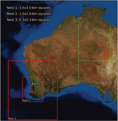
Three nested limited area models were configured to have grid spacings of ~4 km (0.036°), 1 km (0.01°) and 300 m (0.0028°). Fig. 1 shows the nest domains. A fourth nest with a grid spacing of 100 m (0.0009°) was tested; however, simulations at 100-m resolution were not continued because our analysis showed limited value compared to the 300-m domain despite the extra computational expense (a finding consistent with Toivanen et al. 2018). The fire model was switched on and coupled to the atmospheric model for Nest 3. The configuration of the UM is for nests to run to completion sequentially, so two-way fire coupling only occurs on the innermost nest. This may create inconsistencies between the outer and inner domains; however, it is a constraint of the UM nesting suite framework.
ACCESS‐Fire model-run nests at Warona, WA, with the three nests for the simulations shown as red rectangles. Fire coupling is enabled only within the highest resolution nest (N3) at 300 m.
We encountered major problems with model stability in our initial simulations due to numerical stability being sensitive to the boundary layer settings. Frequent model ‘crashes’ occurred, particularly around the time of pyroCb development. Available guidelines were followed, in consultation with UK Met Office colleagues and in combination with trial and error to make several adjustments to the UM science settings. We found that in order to achieve a numerically stable atmosphere when an intense fire is coupled, some non-standard settings were required with the finer resolutions. In addition to those described in Toivanen et al. (2018), the following two boundary layer settings that increased the heat diffusion and momentum mixing were found to be critical: the convective boundary layer stability function needs to be set to ‘standard LEM’; and the ‘transition Ri for sharpest function’ increased from 0.1 to 0.3. Our testing showed that these changes were effective in resolving the numerical stability, although further investigation is required to establish whether there are any unintended consequences resulting from these adjustments.
2.2. Fire model
The code for the fire model is in the UM source tree for the land surface model JULES. Calls to fire-specific subroutines are in the source file sf_impl2_jls.F90. The orography used in the fire model is the 3arcsecond data from the Shuttle Radar Topography Mission (https://earthexplorer.usgs.gov/).
Several changes were made to the original fire code and UM configuration of Toivanen et al. (2018) for the Waroona simulations and some new features were included. A summary of these modifications follows:
the hard-coded switch to turn on/off the calls to the fire-specific subroutines has been replaced by a switch for specific parameters (such as the resolution of the nested domain)
a user-defined polygon option has been introduced to enable start of fire simulation at any time (e.g. from a known fire perimeter after 36 h), this is in addition to circle and line options for initial fire shape
code has been included to enable automatic model restarts and maintain time consistency
a test has been included to check if a grid point is land or water (sea or lake) to prevent the simulated fire from burning across water.
A change was made in the temperature input to the fire code. In general, for fire spread models, the temperature and relative humidity are meant to be measured in the fire-unaffected environment. The coupled model often produces local temperatures of several hundred degrees, therefore using fire-adjacent values to calculate fire spread would introduce a large error. Toivanen et al. (2018) took the approach of averaging the temperature over a 2 × 2-km box and using grid-point relative humidity. Our experiments showed that this approach may still lead to unrealistic temperature and relative humidity values. We found a simple strategy worked better: the environment temperature was taken from the minimum temperature for the sub-domain of each individual processor (a 7 × 7-km box in the case of Nest 3) and the relative humidity taken from the maximum value in the same sub-domain.
The two-dimensional fire spread simulation currently occurs on a subgrid of the ACCESS grid resolution and at more frequent time increments. The fireline spread is calculated by a level set function on the subgrid so that all the fuel in a grid cell does not ignite at once. It has two main components at each time step: (1) calculate fire spread rate and the area in each grid cell that is enclosed by the fire perimeter (the burning area) and (2) calculate the rate of sensible heat release and moisture flux from the amount of fuel burned and pass these energy fluxes to the atmospheric model. Using this framework, the speed at which a fire boundary progresses and the energy released may be substituted with any (empirical) fire spread model for which input data are available.
Fire spread rate was calculated using the DEFFM, see Appendix 1 for the formula for the period 12:00 to 17:00 hours (from Gould et al. 2007). Fuel inputs appropriate for the Waroona area of Western Australia were set in consultation with Dr Lachlan McCaw (pers. comm., 2018). The values used to calculate the DEFFM fire spread were surface fuel hazard score 3.5, near-surface fuel hazard score 2.5 and near-surface fuel height 20 cm. Fuel load was set as a constant 20 Mg ha−1 for our simulations. Homogeneous fuels were used, which was considered to be a sufficiently accurate representation for the continuous fuel on and near the base of the scarp. The assumption of constant fuel is less accurate for fire spread over the coastal plain, but is considered acceptable for our simulations due to the focus on examining the periods of extreme fire behaviour that occurred while the fire was contained to the forested area along and adjacent to the scarp.
3.Results
3.1. Fire line progression
Fire ignition was made as a point ignition at 20:00 hours UTC 5 January (04:00 hours WST on 6 January, local time is Western Standard Time, WST), following the reconstruction of McCaw et al. (2016). Fire ignition on 7 January was made from a polygon perimeter taken from the fire reconstruction at 06:45 hours UTC (14:45 hours WST); this was done to provide a perimeter that started in approximately the correct position to resolve the evening fire spread. The polygon approach implemented here is an improvement to the existing point and line ignition options, but it remains a crude representation of variable fire intensity, self-extinguishment and suppression that occurs around an active fire line.
Fig. 2 shows a comparison of the fire reconstruction from McCaw et al. (2016) and the simulated fire perimeter. The pink isochrones in Fig. 2a show spread to the west in the easterly wind regime on 6 January. As with the Kilmore East simulations described in Toivanen et al. (2018), accurate representation of the perimeter on 6 January was only achieved when spot ignitions identified in the reconstruction were included as new ignition points in the simulation. Our early simulation that did not contain spot ignitions resulted in a fire perimeter that was too slow in arriving at the town of Waroona compared to the reconstruction and consequently did not produce the fire and atmosphere interactions shown in the ember transport section.
(a) Reconstructed fire spread from McCaw et al. (2016). Red contours show 6 January, orange contours show 7 January and grey area shows final perimeter. (b) Hourly isochrones of fire spread from ACCESS-Fire simulation in pink initialised at 04:00 hours WST on 6 January (including spot ignitions) and in orange initialised at 14:45 hours WST on 7 January.

The orange isochrones on 7 January in Fig. 2b show fire spread from a simulation initialised at 11:00 hours WST, with the fire ignited from a polygon at 14:45 hours WST. The polygon was mapped from the fire reconstruction and intended to position the fire front near the base of the scarp leading into the second evening ember storm. The orange isochrones reproduce the slower fire spread in the late afternoon (when the Forest Fire Danger Index, FFDI, peaked), then show acceleration of fire spread down the escarpment towards the town of Yarloop during the evening as the wind speed above the surface increased.
The simulated fire spread for both days is a reassuringly good match for the reconstruction, particularly on 6 January, when the simulated and reconstructed fire perimeter at midnight are in reasonable agreement after ~20 h of simulation time. The simulated perimeter is a poorer match to the reconstruction over the coastal plain, which can be attributed in part to the fire suppression and mitigation efforts that occurred in real time (but which are not included in the simulation), as well as the limitations of constant forest fuels applied over what in reality was mixed farmland.
3.2. Local meteorology
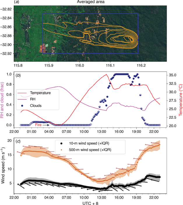
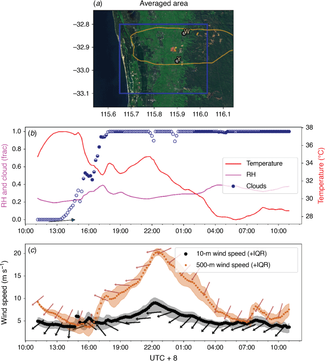
The meteorology of the first 2 days of the Waroona fire is described in detail in the case study (Peace et al. 2017), so the focus here is on features of the simulations. Figures 3 and 4 show simulated meteorological variables on 6 and 7 January respectively. These are averaged over a domain surrounding the fire of Nest 3 to represent conditions unaffected by the fire. Both 6 and 7 January experienced hot maximum temperatures and high overnight minimum temperatures, with low (but not extreme) relative humidity. Easterly near-surface winds prevailed on both days, with a decrease in temperature in the mid-afternoon associated with the sea breeze influence on the western side of the domain.
Selected simulated weather parameters 22:00 hours WST 5 January to 22:00 hours WST 6 January. (a) Blue box shows the domain that weather parameters are averaged over and isochrones of fire spread. (b) Temperature (red), cloud fraction (blue) and relative humidity (pink), ‘Fire’ annotation indicates simulated fire ignition. (c) Wind speed at 10 m (black) and 500 m (beige) arrows indicate wind direction and shading indicates spatial interquartile range.
Selected simulated weather parameters from 10:00 hours WST on 6 January to 10:00 hours WST on 7 January (note the time series start time is different to the previous figure). (a) Blue box shows the domain that weather parameters are averaged over and isochrones of fire spread. (b) Temperature (red), cloud fraction (blue) and relative humidity (pink). (c) Wind speed at 10 m (black) and 500 m (beige), arrows indicate wind direction and direction shading indicates interquartile range.
3.3. Pyrocumulonimbus on 6 January
The pyroCb over the Waroona fire on 6 January developed in a conditionally unstable atmosphere with a backing vertical wind shear profile that supported a coherent, rotating convection column (fig. 4 in Peace et al. 2017 shows the Perth radiosonde). The upright structure (not tilted) and rotation of the column were notable features on video taken during the event. The pyroCb developed in the afternoon and persisted into the early evening, by which time the FFDI measured at Dwellingup, the nearest Bureau of Meteorology Automatic Weather Station (AWS) had fallen below 20. During the period the pyroCb was active, the fire burned intensely and produced extensive areas of defoliated forest consistent with active crown fire. Very heavy fuel loads in long-unburned vegetation were a significant factor in driving the high energy release during the afternoon and lightning ignition of new fires downwind was reported.
The simulations with ACCESS-Fire produce deep moist convective cloud above the fire front, consistent with pyroCb (ACCESS does not support lightning generation). The simulated pyroCb extends through a significant depth of the atmosphere with a vertical extent from ~4.5 km to nearly 15 km in height and with an anvil-like structure in the upper levels. The simulation is otherwise free of deep convective cloud, which is consistent with satellite data during the event. Strong updrafts and downdrafts are produced, with a maximum updraft strength of 30 m s−1, consistent with in-situ measurements reported by Rodriguez et al. (2020) of maximum updrafts of 58 m s−1 at the Pioneer fire in Idaho. The simulated cloud develops at ~14:00 hours WST in the afternoon and dissipates from 19:00 hours WST in the evening. This is broadly consistent with the observations reported in Peace et al. (2017) of overshooting pyrocumulus cloud at 15:30 hours WST and lightning strikes occurring between 16:12 and 20:38 hours WST. Figure 3 shows an increase in wind speed in the evening at 500-m elevation, which likely produces the decrease in cloud cover through tilting and weakening of the low-level updraft.
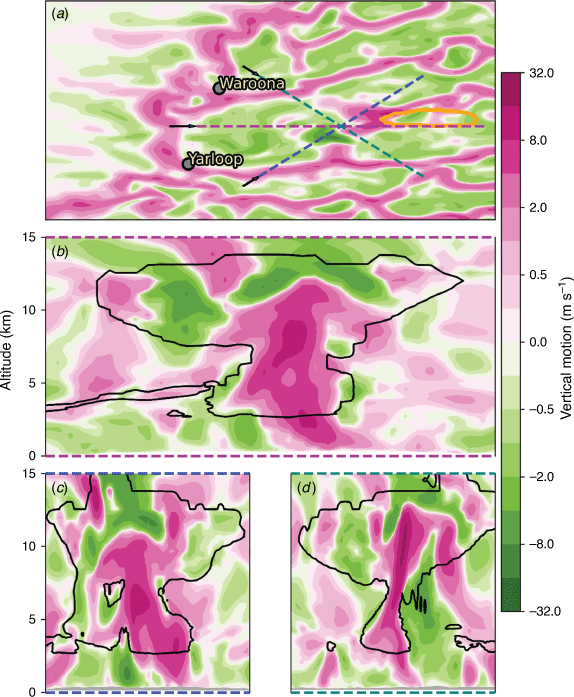
Figure 5 shows horizonal cross sections of vertical wind speed and cloud (ice and water content) above the fire. Coherent regions of ascent and descent, indicating boundary layer convection, are apparent in the lowest 2–3 km, with a shallow layer of scattered cloud simulated at the top of the boundary layer. The fire plume has substantially the strongest updraft at these levels. Above the boundary layer, the fire plume extends a strong, coherent updraft to the stratosphere. This updraft is surrounded by cloud, which narrows as it ascends through the lower troposphere, before broadening into an anvil-like structure. The core updraft is surrounded by concentric rings of weaker descent and ascent, which appear to be a gravity wave response to the buoyant updraft. The simulated gravity wave is consistent with the cirriform anvil seen in time-lapse photography of the pyroCb taken by Darren McCagh of Farmhouse films, a still of which is shown as fig. 7 in Peace et al. (2017).
Cross section of vertical motion (m s−1) at 14:30 hours WST on 6 January (pink, up) on model levels with increasing altitude (top left to bottom right as annotated). Grey dots show Waroona and Yarloop, the blue star shows AWS. The red contour shows the fire perimeter and the red star shows ignition location. The black outline shows cloud as the sum of liquid water and ice content above 0.1 g kg−1.
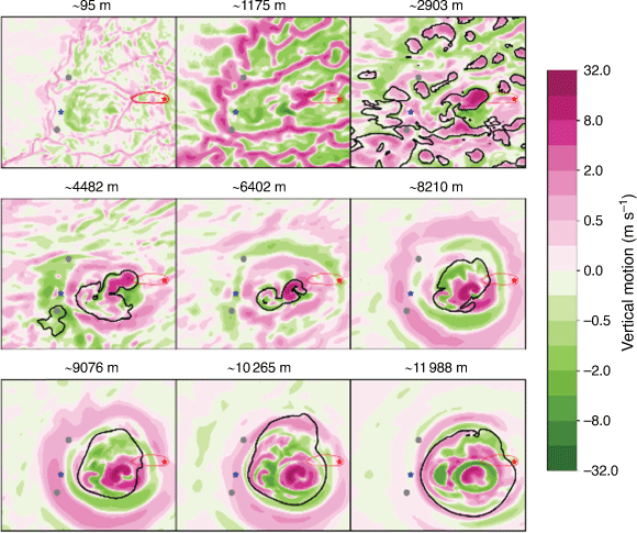
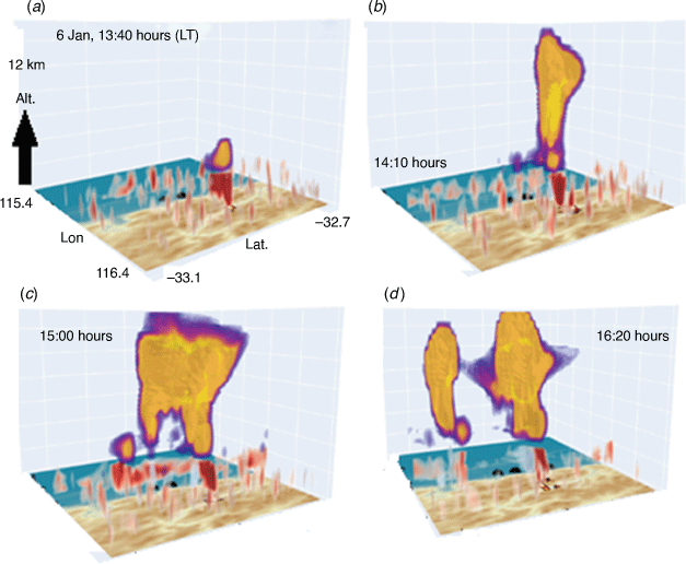
Figure 6 shows three cross sections through the core of the cloud, showing a strong vertical updraft extending upwards from the fire into the cloud base. The updraft accelerates above ~5-km altitude, likely due to additional buoyancy from glaciation of the cloud droplets which may be investigated in future studies with ACCESS-Fire. A three-dimensional visualisation of cloud water and ice, together with vertical motion, for several time steps during the pyroCb lifetime is shown in Fig. 7. From its initial formation at 13:40 hours WST, the cloud grows rapidly upwards to reach full tropospheric extent by 14:10 hours WST. The initial cloud then moves off from the main fire plume, indicated by the deep red shading in the lowest few kilometres, by 15:00 hours WST, but the fire generates a second cloud. By 16:20 hours WST, the cloud to the south (the left in this image) has weakened, but a stronger second cloud remains coupled to the plume updraft.
(a) Plan view showing the fire front (orange contour), vertical motion averaged through an elevated layer 468–1633 m (pink, up; green, down) and location of cross sections in b–d (dashed lines) at 14:30 hours WST on 6 January. b–d show cross sections (see dashed lines in top panel: red is centre panel, green shows bottom right and blue bottom left) showing vertical motion, and cloud (black contour on 0.1 g kg−1 ice and water content).
Three-dimensional visualisation of cloud structure and fire heat release over four times steps: 13:40, 14:10, 15:00 and 16:20 hours WST left to right and top to bottom, looking from the southeast to the northwest. Dimensions in x, y and z are longitude, latitude and altitude above ground level respectively. Purple to yellow shading shows cloud content as liquid water and ice content above 0.1 g kg−1. Red and blue shading shows vertical motion between 3 and 6 m s−1 up to 2-km altitude above ground level. Near the surface black–red–yellow shading is shown for potential temperature greater than 311 K, where fire heat release is highest. Ground level shows a teal to brown filled contour surface of altitude; teal largely represents the coastal plain and brown the region to the east of the escarpment.
3.4. Ember storm
Community impacts from the fire were particularly felt due to the ember showers and mass spotting events on both evenings. On 6 January a ‘sustained ember attack’ was reported at Waroona at 21:00 hours WST and the following evening on 7 January an ember storm affected Yarloop between 19:00 and 20:30 hours WST.
The fire ground reports did not describe isolated embers resulting from long-range spotting, but mass spotting consistent with large numbers of embers transported over a comparatively short distance. In the case study (Peace et al. 2017) we proposed that a low-level wind maximum and hydraulic jump adjacent to the scarp interacted with the fire plume and that this was a contributing mechanism to localised turbulent wind flow and the observed mass spotting. Both towns are located near the base of the scarp and the area is a known location for gusty winds (locally known as ‘scarp winds’) during the evening and overnight. Detailed observations of the development of mountain waves and strong, gusty surface winds in easterly flow over the scarp were presented by Pitts and Lyons (1989) and modelled by Pitts and Lyons (1990) and Blockley and Lyons (1994).
Figures 3 and 4 show the simulated surface and elevated wind speed. The temporal variability in wind speed at an elevation of ~500 m is a feature of both days, with the minimum at both levels occurring mid-afternoon and the maximum in the evening, but the difference being much greater at 500 m. This temporal maximum in wind speed is out of phase with the typical diurnal cycle of fire risk, which is expected to peak in the mid-afternoon. The increase in wind speed at 500 m from late afternoon, reaching a maximum during the evening, coincides with the timing of the two mass spotting events. Figures 3 and 4 show that the increase in wind speed at 500-m elevation is not reflected in the mean 10-m wind, which reconciles with expected diurnal boundary layer processes and development of a nocturnal temperature inversion in the absence of an active fire.
Our simulations provide insights into the plume and wind interactions on the first evening, as they show the winds at ~500 m were entrained by the fire plume and the resulting fire spread occurred in response to the stronger winds above the surface. Figure 8 shows heat flux (an indicator of fire intensity, note the log scale) for the coupled and uncoupled simulations at 21:20 hours WST on 6 January. The simulated fire intensity is much higher in the coupled run and the fire has progressed further to the west, because of the coupling process producing faster fire spread during the early evening. The fire in the uncoupled plot has spread from the spot fire ignition that was included using time and location taken from the reconstruction and the main fire is located near the eastern boundary. In the coupled simulation the spot and the main fire have merged. The streamlines in the coupled plot show higher wind speeds in the vicinity of the fire front as well as convergence into the head fire, with the modification in wind direction extending some distance from the fire. The key mechanism for the faster surface fire spread in the coupled run is the fire’s response to the stronger elevated winds being brought to the surface, whereas in the uncoupled run the much lighter 10-m winds drive the surface fire spread (see Fig. 3). This increase in fire intensity and spread speed from coupling is compelling, because the observed increase in fire activity in the evening was unexpected and contrary to expectations of diurnal fire activity.
Simulated fire intensity (yellow–red, log scale), topography (shaded green–brown) and streamlines at 21:20 hours WST on 6 January for the coupled (top) and uncoupled (bottom) runs. Wind speed is indicated by the thickness of the streamlines. Yellow and blue dashed lines indicate the location of transects in Fig. 9.
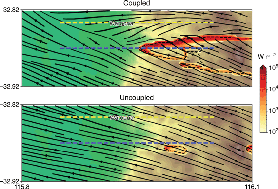
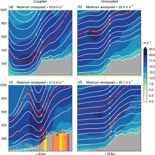
Figure 9 shows vertical cross sections of the low-level wind structure for coupled (left) and uncoupled (right) simulations as the fire burned down the scarp on 6 January. The time of the plot is 21:20 hours WST, which matches the time of ember shower reports at Waroona. An animation at 10-min increments (our output timesteps) shows that the process persists for several timesteps, but the detail of the structure changes. The coupled simulation in Fig. 9 shows three distinct features that differ from the uncoupled version. The first is that the coupling brings the jet (wind) maximum closer to the surface, increasing the near-surface winds and hence the surface fire spread. The second is that the elevated maximum wind speeds are faster in the coupled simulations, with the series of plots (not all shown) having maximum mean wind speeds ~80 km h−1 coincident with or just ahead of the leading edge of the fire perimeter within a few hundred metres of the surface and within the plume circulation. Third, the streamlines show a wave structure and the potential temperature lines are perturbed near the base of the scarp. These features provide a localised lifting mechanism and imply strong turbulence and are therefore processes resolved in the simulated fire–atmosphere interactions that are consistent with the descriptions of the ember shower over the town of Waroona.
Cross sections along the two transects shown in Fig. 8 at 21:20 hours WST on 6 January. Left plots show fire coupling enabled, right plots have no coupling between the fire and atmosphere. Blue shading shows wind speed (m s−1), white lines show streamlines, dashed lines (red and orange) show potential temperature and orange–pink shaded vertical bars show approximate position of fire superimposed on grey topography.
4.Discussion and conclusions
This study describes simulations of the Waroona fire using the coupled fire–atmosphere model ACCESS-Fire. The investigation focusses on two features of the first day, the development of pyroCb and the vertical wind structure interacting with the fire plume when an ember storm occurred, as well as presenting a comparison of the simulated and reconstructed fire perimeter. The simulation results with ACCESS-Fire using the DEFFM fuel model are a good match for the reconstructed fire perimeter. We consider that the fire spread perimeter would be ‘good enough to be useful’ as operational guidance. Importantly in an operational context, the temporal and spatial details show periods of rapid fire spread and high intensity fire in response to coupling with above-surface winds at an elevation of ~500 m. This guidance would provide useful preparedness and planning information for identifying critical time periods for fast fire runs. The features of interest that are resolved in the pyroCb and surrounding the ember storm result from processes in the vertical structure of the atmosphere and the fire plume; processes that would not be apparent from an assessment of uncoupled near-surface meteorological fields.
The DEFFM fire spread model that was used in these simulations has not previously been implemented in a coupled fire–atmosphere model. The fuel settings we used were realistic, and no adjustments or calibrations were made to the fire model settings. For the periods when the assumption of constant fuels is valid, the simulated perimeter shows a reasonable match with the fire spread reconstruction. These results using the DEFFM with ACCESS-Fire are encouraging, although experiments on other fires are required to make general statements on accuracy.
Planned model developments include heterogeneous fuel types and fuel loads. It is conceptually possible to include the code for any fire spread fuel model in ACCESS-Fire and work is underway to include the eight fuel categories and mapping that are included in the new national Australian Fire Danger Rating System (AFDRS) described in Matthews et al. (2019). The accuracy and validity of ACCESS-Fire is expected to improve once this more detailed spatial fuel information is included.
The simulation produces deep moist convection that has features consistent with the observed pyroCb. The timing, location and vertically coherent structure of the simulated cloud are a good match for the observations. Experiments with varying configurations in both the UM and fire components of ACCESS-Fire were tested in order to balance model numerical stability and production of deep moist convection above the simulated fire. Further systematic testing is required to establish the sensitivity surrounding numerical stability of the UM boundary layer to the heat fluxes produced in ACCESS-Fire and to the production of deep moist convection.
Owing to the impacts of intense fires that generate pyroCb, it is presently of great interest to Australian fire agencies and fire meteorologists. Further research is required to comprehensively understand the fire activity and meteorological environments that produce pyroCb, and the results shown here demonstrate that ACCESS-Fire presents a learning tool that can be used to explore the continuum of processes that produce deep moist convection above a fire. Follow-up research on the nature of feedbacks from deep moist convective processes such as wind gusts onto a fireground would be beneficial to further understanding of potential risks and hazards relevant to firefighter safety. Such work will respond to the strong desire from fire agencies to develop predictive methods that anticipate the spectrum of high-impact fire behaviour in environments favourable for pyroCb. This will provide information that is not included in the surface-based fire spread models that are currently used in operations.
ACCESS-Fire produced fast fire spread and higher intensity fire in response to elevated winds, coincident with the timing of the reported ember shower. Gusty, topographically driven winds in the evening are a known phenomenon in the area in an easterly air stream. However, examination of the simulations shows the increase in fire spread and consequently simulated fire intensity does not occur in response to the environmental surface winds but results from interaction of the fire plume with the low-level wind maximum at ~500-m elevation. Localised vertical motion, turbulence and faster wind speed near the surface result from these interactions. The simulated vertical motion and turbulent winds in the lowest kilometre of the atmosphere produce favourable conditions for localised ember transport. These features would not be identified from an assessment of surface meteorology fields or resolved in uncoupled three-dimensional NWP fields.
The results show that fire and atmosphere interactions adjacent to lee slopes in a downslope wind regime can produce favourable conditions for rapid fire spread and mass spotting. This key finding from the simulations has implications for firefighting and suppression tactics at other locations that are similarly favourable for downslope winds. Two potential avenues for future work are apparent from this finding. The first is development of methods that identify areas conducive to downslope winds and consequently ember transport and rapid fire spread (if a fire is present). A tool could be developed that interrogates high resolution NWP to assess the temporal and spatial variability in low-level atmospheric stability and elevated wind speed maxima over and adjacent to steep topography. The second avenue is research to explore the conditions favourable for short distance mass ember transport, as distinct from long-range spotting. Complimentary use of ACCESS-Fire and Large Eddy Simulation models to examine topographically driven flows and plume trajectories for a given ember burnout time presents a pathway to develop short-distance ember transport parameterisations that could be used for manual fire predictions or be included as a module of (uncoupled) fire simulation models.
There has been significant effort invested to achieve the current capability with ACCESS-Fire, but it is not a mature model, and to date has not received sufficient testing for operational use. Testing of the changes for these simulations has been limited and more rigorous validation is necessary to establish reliability of the current configuration. In presenting the current work, we aim to show that ACCESS-Fire resolves processes associated with extreme fire behaviour to a useful extent, to support the case that there are benefits in further development and use of the model. We also aim to share the qualitative findings with the fire-practitioner community, in order to promptly communicate potential risks at going fires.
Planned future activities will make the code available to a wider research community, with the intent that further model development may occur and that this will contribute to our capacity to predict and respond to hazardous fires. Plans for future code development include improving ignition representation around a fire in progress. The success of the polygon ignition approach shows that future experiments may be performed using known fire perimeters as initial conditions, including potential for spatially variable initialisation using line scan imagery. Ember transport is not currently incorporated in ACCESS-Fire (although short-distance spotting is implicit in the DEFFM model) and is intended for future work. Other planned future improvements include (but are not limited to) inclusion of a smoke and chemistry scheme and systematic testing and validation of UM boundary layer parameterisation settings. Several of the activities listed above are in progress or are under discussion.
The ACCESS-Fire framework is useful for examining landscape-scale case studies. It is unlikely to be advantageous and present a cost–benefit return compared to uncoupled fire simulations for all fires and it is most likely to be useful for large or high-risk fires in complex topography with heavy fuel loads. Further testing is required on a range of cases to demonstrate the appropriate circumstances for use, and more detailed validation is required; however, the results presented here show the potential value of the model. Coen (2018) discussed a range of factors that need to be considered in future development and use of coupled fire–atmosphere models such as ACCESS-Fire. It is intended that publication of this narrowly scoped work will provide impetus for further studies and model development by a wider research community, in order to meet the appetite in Australia for an operational coupled fire–atmosphere modelling capability linked to our national weather prediction framework. Such a tool is needed to mitigate the impacts of more frequent, larger and damaging fires in a changing climate.
Acknowledgements
The authors thank the several reviewers who have provided helpful comments on versions of the manuscript.
References
Blockley JA, Lyons TJ (1994) Airflow over a two-dimensional escarpment. III: nonhydrostatic flow. Quarterly Journal of the Royal Meteorological Society 120(515), 79-109.
| Crossref | Google Scholar |
Clark TL, Jenkins MA, Coen J, Packham D (1996) A coupled atmosphere–fire model: convective feedback on fire-line dynamics. Journal of Applied Meteorology 35, 875-901.
| Crossref | Google Scholar |
Coen J (2018) Some requirements for simulating wildland fire behavior using insight from coupled weather—wildland fire models. Fire 1, 6.
| Crossref | Google Scholar |
Coen JL, Cameron M, Michalakes J, Patton EG, Riggan PJ, Yedinak KM (2013) WRF-Fire: coupled weather–wildland fire modeling with the weather research and forecasting model. Journal of Applied Meteorology and Climatology 52(1), 16-38.
| Crossref | Google Scholar |
Dowdy AJ, Fromm MD, McCarthy N (2017) Pyrocumulonimbus lightning and fire ignition on Black Saturday in southeast Australia. Journal of Geophysical Research: Atmospheres 122(14), 7342-7354.
| Crossref | Google Scholar |
Dowdy AJ, Ye H, Pepler A, Thatcher M, Osbrough SL, Evans JP, Di Virgilio G, McCarthy N (2019) Future changes in extreme weather and pyroconvection risk factors for Australian wildfires. Scientific Reports 9, 10073.
| Crossref | Google Scholar |
Filippi J-B, Bosseur F, Pialat X, Santoni P-A, Strada S, Mari C (2011) Simulation of coupled fire–atmosphere interaction with the MesoNH-ForeFire models. Journal of Combustion 2011, 1-13.
| Crossref | Google Scholar |
Fromm M, Tupper A, Rosenfeld D, Servranckx R, McRae R (2006) Violent pyro-convective storm devastates Australia’s capital and pollutes the stratosphere. Geophysical Research Letters 33(5), L05815.
| Crossref | Google Scholar |
Kablick GP, Allen DR, Fromm MD, Nedoluha GE (2020) Australian PyroCb smoke generates synoptic-scale stratospheric anticyclones. Geophysical Research Letters 47(13), e2020GL088101.
| Crossref | Google Scholar |
Koo E, Pagni PJ, Weise DR, Woycheese JP (2010) ‘Firebrands and spotting ignition in large-scale fires’. International Journal of Wildland Fire 19, 818-843.
| Crossref | Google Scholar |
Mandel J, Beezley JD, Kochanski AK (2011) Coupled atmosphere-wildland fire modeling with WRF 3.3 and SFIRE 2011. Geoscientific Model Development 4, 591-610.
| Crossref | Google Scholar |
McRae RHD, Sharples JJ (2013) A process model for forecasting conditions conducive to blow-up fire events. In ‘20th International Congress on Modelling and Simulation (MODSIM2013)’, 1–6 December 2013, Adelaide, SA, Australia. (Modelling and Simulation Society of Australia and New Zealand) 10.36334/modsim.2013.a3.mcrae
Peace M, McCaw L, Santos B, Kepert JD, Burrows N, Fawcett RJB (2017) Meteorological drivers of extreme fire behaviour during the Waroona bushfire, Western Australia, January 2016. Journal of Southern Hemisphere Earth Systems Science 67(2), 79-106.
| Crossref | Google Scholar |
Pitts RO, Lyons TJ (1989) Airflow over a two-dimensional escarpment. I: observations. Quarterly Journal of the Royal Meteorological Society 115(488), 965-981.
| Crossref | Google Scholar |
Pitts RO, Lyons TJ (1990) Airflow over a two-dimensional escarpment. II: hydrostatic flow. Quarterly Journal of the Royal Meteorological Society 116(492), 363-378.
| Crossref | Google Scholar |
Puri K, Dietachmayer G, Steinle P, Dix M, Rikus L, Logan L, Naughton M, Tingwell C, Xiao Y, Barras V, Bermous I, Bowen R, Deschamps L, Franklin C, Fraser J, Glowacki T, Harris B, Lee J, Le T, Roff G, Sulaiman A, Sims H, Sun X, Sun Z, Zhu H, Chattopadhyay M, Engel C (2013) Implementation of the initial ACCESS numerical weather prediction system. Australian Meteorological and Oceanographic Journal 63, 265-284.
| Crossref | Google Scholar |
Rodriguez B, Lareau NP, Kingsmill DE, Clements CB (2020) Extreme pyroconvective updrafts during a megafire. Geophysical Research Letters 47(18), e2020GL089001.
| Crossref | Google Scholar |
Sharples JJ, Cary GJ, Fox-Hughes P, Mooney S, Evans JP, Fletcher M-S, Fromm M, Grierson PF, McRae R, Baker P (2016) Natural hazards in Australia: extreme bushfire. Climatic Change 139, 85-99.
| Crossref | Google Scholar |
Storey MA, Price OF, Bradstock RA, Sharples JJ (2020) Analysis of variation in distance, number, and distribution of spotting in southeast Australian Wildfires. Fire 3(2), 10.
| Crossref | Google Scholar |
Toivanen J, Engel CB, Reeder MJ, Lane TP, Davies L, Webster S, Wales S (2018) Coupled atmosphere–fire simulations of the Black Saturday Kilmore East wildfires with the Unified Model. Journal of Advances in Modeling Earth Systems 11(1), 210-230.
| Crossref | Google Scholar |
Walters D, Boutle I, Brooks M, Melvin T, Stratton R, Vosper S, Wells H, Williams K, Wood N, Allen T, Bushell A, Copsey D, Earnshaw P, Edwards J, Gross M, Hardiman S, Harris C, Heming J, Klingaman N, Levine R, Manners J, Martin G, Milton S, Mittermaier M, Morcrette C, Riddick T, Roberts M, Sanchez C, Selwood P, Stirling A, Smith C, Suri D, Tennant W, Vidale PL, Wilkinson J, Willett M, Woolnough S, Xavier P (2017) The Met Office Unified Model Global Atmosphere 6.0/6.1 and JULES Global Land 6.0/6.1 configurations. Geoscientific Model Development 10, 1487-1520.
| Crossref | Google Scholar |
Wang H (2006) Ember attack: its role in the destruction of houses during ACT bushfires in 2003. In ‘10th Biennial Australasian Bushfire Conference: “Life in a fire prone environment–translating science into practice”’, 6–9 June 2006, Brisbane, Qld, Australia. (CSIRO Manufacturing & Infrastructure Technology: Sydney, NSW, Australia). Available at https://www.fireandbiodiversity.org.au/images/publications/conference-2006/Ember_Attack_Its_role_in_the_destruction_of_houses_during_ACT_bushfire_in_2003.pdf
Werth PA, Potter BE, Clements CB, Finney MA, Goodrick SL, Alexander ME, Cruz MG, Forthofer JA, McAllister SS (2011) Synthesis of knowledge of extreme fire behavior: volume I for fire managers. General Technical Report PNW-GTR-854, USDA Forest Service, Pacific Northwest Research Station, Portland, OR, USA.
Appendix 1
The DEFFM CSIRO Forest (Project Vesta) equations, as used in this project, are as follows (Gould et al. 2007; Cruz et al. 2015).
The moisture coefficient (MC), appropriate for sunny afternoons in the warmer months, is given as follows:
where RH is the relative humidity and T is the temperature (°C).
The fuel moisture function follows:
The rate of spread, R (m h−1), is then given as follows:
where U10 is the average 10-m open wind speed (km h−1), FHSs and FHSns are the fuel hazard scores for surface and near-surface fuels respectively, Hs is the surface fuel height and B1 = 1.03 is a correction for model bias.