
Sea surface height trends in the southern hemisphere oceans simulated by the Brazilian Earth System Model under RCP4.5 and RCP8.5 scenarios
Emanuel Giarolla A F , Sandro F. Veiga B C , Paulo Nobre C , Manoel B. SilvaA Centre for Weather Forecast and Climate Studies, Brazilian National Institute for Space Research (CPTEC/INPE), São José dos Campos, SP, Brazil.
B Earth System Science Centre, Brazilian National Institute for Space Research (CCST/INPE), São José dos Campos, SP, Brazil.
C Centre for Weather Forecast and Climate Studies, Brazilian National Institute for Space Research (CPTEC/INPE), Cachoeira Paulista, SP, Brazil.
D Amazonas State University, Manaus, AM, Brazil.
E University of Potsdam, Potsdam, Germany.
F Corresponding author. Email: egiarolla@yahoo.com.br
Journal of Southern Hemisphere Earth Systems Science 70(1) 280-289 https://doi.org/10.1071/ES19042
Submitted: 27 August 2019 Accepted: 13 July 2020 Published: 8 October 2020
Journal Compilation © BoM 2020 Open Access CC BY-NC-ND
Abstract
The Brazilian Earth System Model (BESM-OA2.5), while simulating the historical period proposed by the fifth phase of the Coupled Model Intercomparison Project (CMIP5), detects an increasing trend in the sea surface height (SSH) on the southern hemisphere oceans relative to that of the pre-industrial era. The increasing trend is accentuated in the CMIP5 RCP4.5 and RCP8.5 future scenarios with higher concentrations of greenhouse gases in the atmosphere. This study sheds light on the sources of such trends in these regions. The results suggest an association with the thermal expansion of the oceans in the upper 700 m due to a gradual warming inflicted by those future scenarios. BESM-OA2.5 presents a surface height increase of 0.11 m in the historical period of 1850–2005. Concerning future projections, BESM-OA2.5 projects SSH increases of 0.14 and 0.23 m (relative to the historical 2005 value) for RCP4.5 and RCP8.5, respectively, by the end of 2100. These increases are predominantly in a band of latitude within 35–60°S in the Atlantic and Indian oceans. The reproducibility of the trend signal detected in the BESM-OA2.5 simulations is confirmed by the results of three other CMIP5 models.
Keywords: Brazilian Earth System Model, CMIP5, IPCC AR5 scenarios, RCP4.5, RCP8.5, sea level trends, sea surface height, southern hemisphere oceans.
1 Introduction
Due to the societal impact of sea level elevation, especially in coastal regions, many studies on this subject have recently emerged (e.g. Yin 2012; Lyu et al. 2014; Slangen et al. 2014; Durack et al. 2014; Little et al. 2015; Carson et al. 2015; Carson et al. 2016; Dangendorf et al. 2017; among others). Based on observations and simulations of distinct atmosphere–ocean general circulation models from the Coupled Model Intercomparison Project phase 5 (Taylor et al. 2012, referred to as CMIP5), the Fifth Assessment Report (chapter 13, Church et al. 2013, referred to as AR5) of the Intergovernmental Panel on Climate Change (IPCC) concluded that the global sea level rise in the 21st century would likely surpass the increase rate detected for 1971–2010. Such a sea elevation change is observed in all Representative Concentration Pathway (RCP) scenarios due to the expansion of the ocean and the transfer of mass from glaciers and ice sheets. Most of the models used in such studies consistently predict a global sea level increase in future scenarios; however, they show discrepancies in the rate of such increases due to particularities of each model in their representations of the climate system in addition to their inherent internal variability (Little et al. 2015). Therefore, prediction of the sea level in future climate projections benefits from the use of as many models as possible, together with their respective ensemble means (Yin 2012; Carson et al. 2015). The present work adds the coupled atmosphere–land–ocean–sea ice model developed in Brazil (the Brazilian Earth System Model referred to as BESM, Nobre et al. 2013; Veiga et al. 2019; Capistrano et al. 2020) to this effort by evaluating the sea level changes in the southern hemisphere oceans in two RCP scenarios, and considering the effects of ocean thermal expansion on the sea level increase.
The first scenario (RCP4.5) considers a greenhouse gas concentration peak in 2040 with a subsequent decline relative to the pre-industrial value, thus stabilising the radiative forcing at 4.5 W m–2 in the year 2100 (Meinshausen et al. 2011; Thomson et al. 2011). In the second and more dramatic scenario (RCP8.5), the greenhouse gas concentrations increase considerably over time, relative to the pre-industrial value, leading to an increasing radiative forcing of 8.5 W m–2 at the end of 2100 (Riahi et al. 2011). An overall increasing sea level trend is predicted in all southern hemisphere oceans by both scenarios, particularly by RCP8.5, based on the results of previously cited studies. This study focuses on details of the sea level trend in this region.
2 Material and methods
The model used in this study is the Brazilian Earth System Model (Nobre et al. 2013) version ‘ocean–atmosphere–sea ice coupled model 2.5’ (BESM-OA2.5). BESM-OA2.5 includes the ocean model which was developed at the Geophysical Fluid Dynamics Laboratory (GFDL), the Modular Ocean Model version 4p1 (MOM4p1), with a built-in Sea Ice Simulator (SIS), coupled to the spectral atmospheric model which, in its turn, has been developed since the 1990s at the Centre for Weather Forecasting and Climate Studies of the Brazilian National Institute for Space Research (CPTEC/INPE), the Brazilian Atmospheric Model (BAM), with improvements focused on better representation of the atmospheric processes in the tropical regions, especially in South America (Figueroa et al. 2016). The atmospheric resolution is the triangular truncation of spectral coefficients at wave number 62, corresponding to a horizontal grid spacing of approximately 1.875° × 1.875° at the equator, and 28 sigma levels unevenly spaced in the vertical (T62 L28). The ocean model zonal grid resolution is 1° of longitude, and the meridional grid spacing varies uniformly from 1/4° of latitude between the equator and 10°, to 1° at 45° and to 2° at 90° in both hemispheres. The vertical resolution comprises 50 levels with a 10-m resolution in the upper 220 m, increasing gradually to about 370 m in deeper regions (Giarolla et al. 2015). The model characteristics, spin-up process, parameterisation, and the historical run evaluation are described in Veiga et al. (2019), and its sensitivity to radiative forcing is evaluated in Capistrano et al. (2020).
The term ‘sea level’ is generic and needs to be clearly defined (Gregory et al. 2019). In this study, the sea level variable is the MOM4p1 native output ‘eta_t’, which is defined as the ‘surface height on T cells’, where ‘T cells’ are the tracer cells of an Arakawa B-grid (Griffies 2012). In this work, this variable is referred to as ‘sea surface height’ (SSH). A non-Boussinesq (mass conserving) model option was chosen. This model allows changes in the water volume and, therefore, incorporates the steric effect component into the total SSH. BESM-OA2.5 does not include significant mass transfers from land to ocean, such as land ice melting. It does include, however, a parameterised, climatological annual mean river discharge at the main river mouths of all continents, estimated from continental imbalances between precipitation, evaporation, and storage, which are then partitioned among the bordering ocean basins via use of river routing schemes and flow estimates (Large and Yeager 2008). The river mixing process is formulated in terms of tendencies, added to the tracer concentration equation, such that the consequent free surface height changes are handled just they are for other forms of fresh water, such as precipitation and evaporation (Griffies 2012, chapter 28). In this study, we assume that sea level changes due to liquid river runoff have a small impact on the global mean sea level; therefore, they are not considered.
The experiments consider two future RCP scenarios, RCP4.5 and RCP8.5, as mentioned above. Both experiments start from the end of the ‘historical’ experiment, a simulation for 1850–2005 that assumes greenhouse gas rates similar to those observed in the same time period. The outputs were on a monthly basis from January 2006 to December 2100, and they were averaged annually to filter out seasonal variabilities. The geographical region studied here includes all the southern hemisphere oceans within 10–60°S.
To compare the BESM-OA2.5 description of sea level rise changes with those predicted by other models, the variable ‘zos’ of three selected CMIP5 models, i.e. MIROC-ESM (Watanabe et al. 2011), GISS-E2-R (Miller et al. 2014), and NorESM1-M (Bentsen et al. 2013), for RCP4.5 and RCP8.5 are also given in this study. In the CMIP5 table of variables, zos represent the local height of the sea surface above the geoid which, by definition, has a mean of zero. Nevertheless, some models store it with a nonzero time-dependent mean (Gregory et al. 2019), including the models chosen for the comparison with BESM-OA2.5.
3 Results
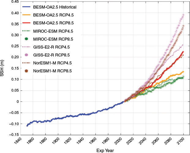
As shown in Fig. 1, the increasing trend in the mean SSH observed in the historical run of BESM-OA2.5 (in the order of approximately 0.11 m) in the southern hemisphere oceans is expanded in both RCP runs, and is especially accentuated in RCP8.5 for most (but not all) models. The RCP4.5 response is similar to that of RCP8.5 for approximately 2006–2040. By 2050, both experiments accumulate an increment of 0.06 m in the mean SSH of the southern hemisphere oceans. In RCP4.5, after 2050, the inflection and subsequent reduction in the increased rate approximately coincides with the greenhouse gas concentration decline in this scenario. In 2100, the curves culminated in increments of 0.137 and 0.226 m for RCP4.5 and RCP8.5, respectively. The equivalent curves from the other CMIP5 models for RCP4.5 and RCP8.5 are also shown in Fig. 1. In Fig. 1, it is noteworthy that (except in the case of MIROC) the RCP8.5 SSH trends rise more steeply than those from the sibling RCP4.5 experiments, as expected based on the larger RCP8.5 radiative/temperature forcing profiles.
|
Fig. 2 shows SSH maps of linear trends from 2006–2100 for the BESM-OA2.5 RCP scenarios. Notwithstanding the overall increasing trend shown in all regions, the latitudinal band 35–60°S stands out in both RCPs, especially in the Indian and Atlantic oceans. In fact, AR5 ensemble maps and analyses suggest that even though the overall sea level trend is positive towards the 21st century, spatial variations may occur among particular seas or ocean basins (AR5). This band of maximum positive linear trend is also present in the results of the other CMIP5 models (Fig. 3). The strengthening of the positive linear trend patterns shown in Fig. 3, along with the increasing radiative forcing from RCP4.5 to RCP8.5 (despite each model having its own particular response in terms of regional and overall trend), are discussed in the next section.

|

|
The trend maps shown in Fig. 3 also complement the information of the SSH time series shown in Fig. 1. For example, in Fig. 3, the GISS-E2-R model has the highest overall linear trend in the 2006–2100 period followed by NorESM1-M. Similarly, both models present the first and the second highest mean SSH anomaly values at 2100 in Fig. 1, followed by BESM-OA2.5, for both the RCP4.5 and RCP8.5 runs. The MIROC-ESM maps, in addition to the positive trend band around 35–60°S (consistent with the other models), present an extensive region of negative trends in the higher latitudes, but the positive trends in the lower latitudes are not as strong as those in the other models; therefore, the MIROC-ESM resultant time series in Fig. 1 show the lowest mean SSH values at 2100.
4 Discussion
Hu and Bates (2018) outlined the major processes controlling global and regional sea level rise: (1) the mass component (oceanic net mass change related to ice sheets and glaciers, groundwater mining, and dam building); (2) the glacial isostatic adjustment (the vertical movement of the earth’s crust due to ice sheet mass changes); (3) the thermosteric and halosteric effects (changes in ocean water temperature and salinity, respectively); (4) changes in the earth’s gravitational field related to the melting of ice sheets; and (5) ocean dynamics (associated with variations in wind- or buoyancy-driven ocean circulation). Because the BESM-OA2.5 version utilised here does not involve continental ice or other hydrological processes that could induce sea level changes (as mentioned before), the main causes of the SSH trends here lie in steric expansion and ocean dynamics.
To investigate steric expansion, the ‘steric height’ component was computed from the BESM-OA2.5 temperature and salinity results from the surface to 700 m via the expression:
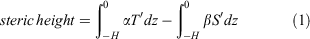
where T′ and S′ are temperature and salinity anomalies, respectively, in relation to the T and S time means, for 2006–2100, related to each RCP experiment. The values of the α (t, x, y, z) and β (t, x, y, z) coefficients were estimated via the same state approximation equation used in MOM4p1, i.e. McDougall, Jackett, Wright, and Feistel’s equation of state (McDougall et al. 2003).
In a qualitative analysis, the linear trend maps estimated using steric heights (Fig. 4a) for each RCP are very similar to those of the total SSH (Fig. 2), especially in the band of higher trends within 35–60°S. These observations are consistent with the other models shown in Fig. 3 and the results presented in AR5 (e.g. figures 13.15 and 13.16, the latter regarding dynamic and steric effects on sea level changes).

|
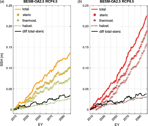
In this model study, the main contributor to the sea level trends in the southern hemisphere oceans is thermal expansion, for the following reasons. First, the heat content trend maps for both RCPs, computed via integration of the temperature anomalies by depth (0–700 m) multiplied by the mean density of the water column and the specific heat of seawater (Fig. 4b), show higher values, especially in the regions also containing the steric height (Fig. 4a) and total SSH (Fig. 2) maxima. Second, the time series of mean steric height (Fig. 5) indicates that the SSH induced only by steric effects would reach a departure value in 2100 of approximately 74.5% (0.102 m) of the total SSH increase for RCP4.5 (0.137 m), with the thermosteric component responsible for only about 55.5% (0.076 m). This effect is clearer in RCP8.5, where the steric SSH departure value in 2100 (0.188 m) is about 83.3% of the total SSH increase (0.226 m), with a 69.6% contribution from the thermosteric component. The halosteric contribution (the right side of Eqn 1) to the SSH increase in 2100 is smaller, as it is responsible for approximately 19.0% and 13.7% of the total SSH increase in the RCP4.5 and RCP8.5 runs, respectively. Furthermore, as stated by Gregory et al. (2019), the halosteric contribution to sea level change on a global scale is practically zero, as the global salt content is conserved.
|
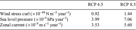
Fig. 5 also shows curves for the differences in the total and the steric SSH anomalies. Such curves represent the influence of other contributors to the overall SSH increase in the southern hemisphere oceans beyond the steric response discussed above. Besides the minimal effects of approximation errors on the steric height estimate, the difference curves in Fig. 5 also represent the ocean dynamics influence, i.e. the wind-induced SSH trends via mass distribution adjustments (Roemmich et al. 2007; Lee and McPhaden 2008). For instance, Han et al. (2010) attribute the regional variations in sea level in the Indian Ocean since the 1960s to changes in surface winds associated with a combined enhancement of Hadley and Walker Cells. As yet another example, the influence of wind changes on the Antarctic Circumpolar Current (ACC), and consequently on the sea level in the southern hemisphere oceans, is summarised by Hu and Bates (2018) and Gregory et al. (2016, 2019) and references therein. A sea level pressure deepening south of the ACC, together with a rising in the southern hemisphere mid-latitudes north of the ACC, cause a strengthening of the westerly winds due to the Coriolis Force in both future scenarios. Thus, the resulting geostrophic balance leads to a stronger ACC (but with an initial slow-down in RCP4.5). This effect, in turn, leads to a larger gradient in SSH across the current, causing the mean sea level to fall south of the ACC and to rise north of the ACC. Hu and Bates (2018) and Gregory et al. (2016) also point out the importance of eddies in ACC dynamics, which are generally not reproduced properly by many CMIP5 models as a result of their coarse ocean resolution in that region. Although the investigation of wind-driven SSH changes is beyond the scope of this study, Fig. 6 depicts how the wind stress curl, sea level pressure, and near surface zonal current (at 5 m depth) change after nearly 100 years in the RCP4.5 scenario, and more intensively in the RCP8.5 scenario. For the latitudinal region around the ACC (37–60°S), the mean linear increase values per year (for 2006–2100) are shown in Table 1.

|
|
5 Final remarks
In scenarios such as RCP4.5 and RCP8.5, increases in the emission and/or concentration of greenhouse gases can have many effects on the atmosphere and in the oceans (AR5; Church et al. 2013). On a global scale, the RCP greenhouse gas emission rates influence the global ocean heat uptake (Church et al. 2013, fig. 13.8). The overall oceans then present a slow and continuous warming over a few decades (e.g. Rind et al. 2018), favouring SSH increases via thermal expansion, i.e. thermosteric SSH trends. The salinity in those scenarios is also affected due to anomalies in the evaporation–precipitation balance, plus the effects of sea ice melt and salt redistribution in the ocean, which induce the halosteric SSH trends. Thermosteric and halosteric components, together with mass transfer from land (e.g. land ice melting), are the main factors responsible for global sea level changes (Hu and Bates 2018). Considering the characteristics of the coupled atmosphere–land–ocean–sea ice model utilised here (BESM-OA2.5), which includes time invariant mass transfers from land to ocean and treats salt as a conservative tracer, it follows that most of the presented sea level changes simulated by the model are caused by thermosteric effects, with possible contributions from fluctuations in ocean dynamics induced by wind stress patterns present in these RCP scenarios.
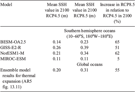
In relation to the steric sea level rise in the southern hemisphere oceans, after a mean increase of approximately 0.11 m during the historical run, BESM-OA2.5 RCP runs predict a mean steric sea level rise of another 0.14 and 0.23 m by 2100 as a result of RCP4.5 and RCP8.5 radiative forcing, respectively. In terms of percentage, the RCP8.5 run shows a mean SSH increase in the southern hemisphere oceans of 65% by 2100 in relation to the increase obtained in the RCP4.5 run (Fig. 1). The relative increases in the steric sea level rise from two of the other CMIP5 models cited in this study also produce similar percentages in the increase rate in 2100 between RCP4.5 and RCP8.5 runs (Table 2). MIROC-ESM, on the other hand, simulated a practically coincident mean sea level rise in the southern hemisphere oceans in 2100 in both RCP scenarios. For comparison, in the time series shown in AR5, which represents the global sea level rise due to thermal expansion (AR5 fig. 13.11), it is possible to infer sea level increment values relative to the 2006 value for RCP4.5 and RCP8.5 (see also Table 2).
|
The BESM-OA2.5 southern hemisphere sea level mean rise prediction assigns sea level trend maxima, which are attributable to thermal expansion, to a band of latitude of 35–60°S in the Atlantic and Indian oceans, and this effect is also apparent in the results from the other three selected CMIP5 models. It is not clear, however, which dynamic/thermodynamic effects contribute to the heat content spatial structure in this band, which shall be addressed in further studies on the subject.
Among all of the studies using the BESM-OA2.5 model as a research tool that have emerged since Nobre et al. (2013), this is the first dedicated to evaluating the sea level variations under RCP forcing scenarios, including comparison with other CMIP5 model runs. The coincident spatial structures from several models in the regions of the maximal mean steric sea level rise in the southern hemisphere documented in this study constitute one of the most notable results shown so far. The ability of BESM-OA2.5, among the other models, to simulate such a feature (beyond the mean sea level rise in the entire southern hemisphere oceans per se) indicates that BESM-OA2.5 is well suited for further climate change studies of the southern hemisphere, which require the model’s capacity to resolve regional-scale oceanic phenomena embedded in a global coupled climate simulation.
Conflicts of interest
The authors declare that they have no conflicts of interest.
Acknowledgements
This work was supported by FAPESP (grant nos. 2009/50528-6, 2014/50848-9, and 2018/06204-0), CAPES (grant no. 16/2014), CAPES/National Water Agency (CAPES/ANA) (grant no. 88887.115872/2015-01), CNPq (grant nos. 490237/2011-8 and 302218/2016-5), FINEP/Rede Clima (grant no. 01.13.0353-00), INCT-MC (grant no. 573797/2008-0), INCT-MC Phase 2 funded by CNPq (grant no. 465501/2014–1), and INPE. Sandro F. Veiga was supported by the Earth League Earth-Doc grant, funded by CAPES (88887.197771/2018-00). Manoel B. Silva Jr. was supported by a grant funded by FAPESP (2018/06204-0). Andyara O. Callegare was supported by the PIBIC/INPE/CNPp grant program. The authors also thank the anonymous reviewers, and Ricardo P. Matano for his suggestions in previous versions of this work.
References
Bentsen, M., Bethke, I., Debernard, J. B., Iversen, T., Kirkevåg, A., Seland, Ø., Drange, H., Roelandt, C., Seierstad, I. A., Hoose, C., and Kristjánsson, J. E. (2013). The Norwegian Earth System Model, NorESM1-M – Part 1: Description and basic evaluation of the physical climate. Geosci. Model Dev. 6, 687–720.| The Norwegian Earth System Model, NorESM1-M – Part 1: Description and basic evaluation of the physical climate.Crossref | GoogleScholarGoogle Scholar |
Capistrano, V. B., Nobre, P., Veiga, S. F., et al. (2020). Assessing the performance of climate change simulation results from BESM-OA2.5 compared with a CMIP5 model ensemble. Geosci. Model Dev. 13, 2277–2296.
| Assessing the performance of climate change simulation results from BESM-OA2.5 compared with a CMIP5 model ensemble.Crossref | GoogleScholarGoogle Scholar |
Carson, M., Köhl, A., and Stammer, D. (2015). The Impact of Regional Multidecadal and Century-Scale Internal Climate Variability on Sea Level Trends in CMIP5 Models. J. Climate 28, 853–861.
| The Impact of Regional Multidecadal and Century-Scale Internal Climate Variability on Sea Level Trends in CMIP5 Models.Crossref | GoogleScholarGoogle Scholar |
Carson, M., Köhl, A., Stammer, D., Slangen, A. B. A., Katsman, C. A., van de Wal, R. S. W., Church, J., and White, N. (2016). Coastal sea level changes, observed and projected during the 20th and 21st century. Climatic Change 134, 269–281.
| Coastal sea level changes, observed and projected during the 20th and 21st century.Crossref | GoogleScholarGoogle Scholar |
Church, J. A., Clark, P. U., Cazenave, A., Gregory, J. M., Jevrejeva, S., Levermann, A., Merrifield, M. A., Milne, G. A., Nerem, R. S., Nunn, P. D., Payne, A. J., Pfeffer, W. T., Stammer, D., and Unnikrishnan, A. S. (2013). Sea Level Change. Pages 1137–1216, In: ‘Climate Change 2013. The Physical Science Basis. Contribution of Working Group I to the Fifth Assessment Report of the Intergovernmental Panel on Climate Change’. (Eds T. F. Stocker, D. Qin, G.-K. Plattner, M. Tignor, S. K. Allen, J. Boschung, A. Nauels, Y. Xia, V. Bex and P. M. Midgley) Cambridge University Press, Cambridge, United Kingdom and New York, NY, USA.
Dangendorf, S., Marcos, M., Wöppelmann, G., Conrad, C. P., Frederikse, T., and Riva, R. (2017). Proc. Nat. Acad. Sci. 114, 5946–5951.
| Crossref | GoogleScholarGoogle Scholar | 28533403PubMed |
Durack, P. J., Wijffels, S. E., and Gleckler, P. J. (2014). Long-term sea-level change revisited: the role of salinity. Environ. Res. Lett. 9, .
| Long-term sea-level change revisited: the role of salinity.Crossref | GoogleScholarGoogle Scholar |
Figueroa, S. N., Bonatti, J. P., Kubota, P. Y., Grell, G. A., Morrison, H., Barros, S. R. M., Fernandez, J. P. R., Ramirez, E., Capistrano, V. B., Alvim, D. S., Enoré, D. P., Diniz, F. L. R., Barbosa, H. M. J., Mendes, C. L., and Panetta, J. (2016). The Brazilian Global Atmospheric Model (BAM): Performance for Tropical Rainfall Forecasting and Sensitivity to Convective Scheme and Horizontal Resolution. Wea. Forecast 31, 1547–1572.
| The Brazilian Global Atmospheric Model (BAM): Performance for Tropical Rainfall Forecasting and Sensitivity to Convective Scheme and Horizontal Resolution.Crossref | GoogleScholarGoogle Scholar |
Giarolla, E., Siqueira, L. S. P., Bottino, M. J., Malagutti, M., Capistrano, V. B., and Nobre, P. (2015). Equatorial Atlantic Ocean dynamics in a coupled ocean–atmosphere model simulation. Ocean Dyn. 65, 831–843.
| Equatorial Atlantic Ocean dynamics in a coupled ocean–atmosphere model simulation.Crossref | GoogleScholarGoogle Scholar |
Gregory, J. M., Bouttes, N., Griffies, S. M., et al. (2016). The Flux-Anomaly-Forced Model Intercomparison Project (FAFMIP) contribution to CMIP6: investigation of sea-level and ocean climate change in response to CO2 forcing. Geosci. Model Dev. 9, 3993–4017.
| The Flux-Anomaly-Forced Model Intercomparison Project (FAFMIP) contribution to CMIP6: investigation of sea-level and ocean climate change in response to CO2 forcing.Crossref | GoogleScholarGoogle Scholar |
Gregory, J. M., Griffies, S. M., Hughes, C. W., et al. (2019). Concepts and Terminology for Sea Level: Mean, Variability and Change, Both Local and Global. Surv Geophys 40, 1251–1289.
| Concepts and Terminology for Sea Level: Mean, Variability and Change, Both Local and Global.Crossref | GoogleScholarGoogle Scholar |
Griffies, S. M. (2012). Elements of the Modular Ocean Model (MOM) (2012 release with updates). GFDL Ocean Group Technical Report No. 7, NOAA/Geophysical Fluid Dynamics Laboratory.
Han, W. Q., Meehl, G. A., Rajagopalan, B., et al. (2010). Patterns of Indian Ocean sea-level change in a warming climate. Nature Geosci. 3, 546–550.
| Patterns of Indian Ocean sea-level change in a warming climate.Crossref | GoogleScholarGoogle Scholar |
Hu, A., and Bates, S. C. (2018). Internal climate variability and projected future regional steric and dynamic sea level rise. Nature Comm. 9, 1068.
| Internal climate variability and projected future regional steric and dynamic sea level rise.Crossref | GoogleScholarGoogle Scholar |
Large, W. G., and Yeager, S. G. (2008). The global climatology of an interannually varying air–sea flux data set. Clim Dyn. 33, 341–364.
| The global climatology of an interannually varying air–sea flux data set.Crossref | GoogleScholarGoogle Scholar |
Lee, T., and McPhaden, M. J. (2008). Decadal phase change in large-scale sea level and winds in the Indo-Pacific region at the end of the 20th century. Geophys. Res. Lett. 35, L01605.
| Decadal phase change in large-scale sea level and winds in the Indo-Pacific region at the end of the 20th century.Crossref | GoogleScholarGoogle Scholar |
Little, C. M., Horton, R. M., Kopp, R. E., Oppenheimer, M., and Yip, S. (2015). Uncertainty in Twenty-First-Century CMIP5 Sea Level Projections. J. Climate 28, 838–852.
| Uncertainty in Twenty-First-Century CMIP5 Sea Level Projections.Crossref | GoogleScholarGoogle Scholar |
Lyu, K., Zhang, X., Church, J. A., Slangen, A. B. A., and Hu, J. (2014). Time of emergence for regional sea-level change. Nature Climate Change 4, 1006–1010.
| Time of emergence for regional sea-level change.Crossref | GoogleScholarGoogle Scholar |
Meinshausen, M., Smith, S. J., Calvin, K. V., Daniel, J. S., Kainuma, M. L. T., Lamarque, J.-F., Matsumoto, K., Montzka, S. A., Raper, S. C. B., Riahi, K., Thomson, A. M., Velders, G. J. M., and van Vuuren, D. (2011). The RCP Greenhouse Gas Concentrations and their Extension from 1765 to 2300. Climatic Change 109, 213.
| The RCP Greenhouse Gas Concentrations and their Extension from 1765 to 2300.Crossref | GoogleScholarGoogle Scholar |
Miller, R. L., Schmidt, G. A., Nazarenko, L. S., et al. (2014). CMIP5 historical simulations (1850–2012) with GISS ModelE2. J. Adv. Model. Earth Syst. 6, 441–478.
| CMIP5 historical simulations (1850–2012) with GISS ModelE2.Crossref | GoogleScholarGoogle Scholar |
McDougall, T. J., Jackett, D. R., Wright, D. G., and Feistel, R. (2003). Accurate and computationally efficient algorithms for potential temperature and density of seawater. J. Atmos. Oceanic Tech. 20, 730–741.
| Accurate and computationally efficient algorithms for potential temperature and density of seawater.Crossref | GoogleScholarGoogle Scholar |
Nobre, P., Siqueira, L. S. P., de Almeida, R. A., Malagutti, M., Giarolla, E., Castelão, G. P., Bottino, M. J., Kubota, P., Figueroa, S. N., Costa, M. C., Baptista, M., Irber, L., and Marcondes, G. G. (2013). Climate Simulation and Change in the Brazilian Climate Model. J. Climate 26, 6716–6732.
| Climate Simulation and Change in the Brazilian Climate Model.Crossref | GoogleScholarGoogle Scholar |
Riahi, K., Rao, S., Krey, V., Cho, C., Chirkov, V., Fischer, G., Kindermann, G., Nakicenovic, N., and Rajaf, P. (2011). RCP 8.5 - A scenario of comparatively high greenhouse gas emissions. Climatic Change 109, 33–57.
| RCP 8.5 - A scenario of comparatively high greenhouse gas emissions.Crossref | GoogleScholarGoogle Scholar |
Rind, D., Schmidt, G. A., Jonas, J., Miller, R. L., Nazarenko, L., Kelley, M., and Romanski, J. (2018). Multi-century instability of the Atlantic Meridional Circulation in rapid warming simulations with GISS ModelE2. J. Geophys. Res. Atmos. 123, 6331–6355.
| Multi-century instability of the Atlantic Meridional Circulation in rapid warming simulations with GISS ModelE2.Crossref | GoogleScholarGoogle Scholar |
Roemmich, D., Gilson, J., Davis, R., Sutton, P., Wijffels, S., and Riser, S. (2007). Decadal Spinup of the South Pacific Subtropical Gyre. J. Phys. Oceanogr. 37, 162–173.
| Decadal Spinup of the South Pacific Subtropical Gyre.Crossref | GoogleScholarGoogle Scholar |
Slangen, A. B. A., Carson, M., Katsman, C. A., van de Wal, R. S. W., Köhl, A., Vermeersen, L. L. A., and Stammer, D. (2014). Projecting twenty-first century regional sea-level changes. Climatic Change 124, 317–332.
| Projecting twenty-first century regional sea-level changes.Crossref | GoogleScholarGoogle Scholar |
Taylor, K. E., Stouffer, R. J., and Meehl, G. A. (2012). An overview of CMIP5 and the experiment design. Bull. Am. Meteorol. Soc. 93, 485–498.
| An overview of CMIP5 and the experiment design.Crossref | GoogleScholarGoogle Scholar |
Thomson, A. M., Calvin, K. V., Smith, S. J., Kyle, G. P., Volke, A., Patel, P., Delgado-Arias, S., Bond-Lamberty, B., Wise, M. A., Clarke, L. E., and Edmonds, J. A. (2011). RCP4.5: a pathway for stabilization of radiative forcing by 2100. Climatic Change 109, 77.
| RCP4.5: a pathway for stabilization of radiative forcing by 2100.Crossref | GoogleScholarGoogle Scholar |
Veiga, S. F., Nobre, P., Giarolla, E., Capistrano, V., Baptista, M., Marquez, A. L., Figueroa, S. N., Bonatti, J. P., Kubota, P., and Nobre, C. A. (2019). The Brazilian Earth System Model ocean–atmosphere (BESM-OA) version 2.5: evaluation of its CMIP5 historical simulation. Geosci. Model Dev. 12, 1613–1642.
| The Brazilian Earth System Model ocean–atmosphere (BESM-OA) version 2.5: evaluation of its CMIP5 historical simulation.Crossref | GoogleScholarGoogle Scholar |
Watanabe, S., Hajima, T., Sudo, K., et al. (2011). MIROC-ESM 2010: model description and basic results of CMIP5–20c3 m experiments. Geosci. Model Dev. 4, 845–872.
| MIROC-ESM 2010: model description and basic results of CMIP5–20c3 m experiments.Crossref | GoogleScholarGoogle Scholar |
Yin, J. (2012). Century to multi-century sea level rise projections from CMIP5 models. Geophys. Res. Lett. 39, L17709.
| Century to multi-century sea level rise projections from CMIP5 models.Crossref | GoogleScholarGoogle Scholar |