
Climatology of wind changes and elevated fire danger over Victoria, Australia
Graham Mills A D , Sarah Harris A B , Timothy Brown C and Alex Chen BA School of Earth, Atmosphere and Environment, Monash University, Clayton, Victoria, Australia.
B Fire and Emergency Management, Country Fire Authority, East Burwood, Victoria, Australia.
C Division of Atmospheric Science, Desert Research Institute, Reno, NV, USA.
D Corresponding author. Email: gam4582@gmail.com
Journal of Southern Hemisphere Earth Systems Science 70(1) 290-303 https://doi.org/10.1071/ES19043
Submitted: 12 April 2020 Accepted: 5 August 2020 Published: 8 October 2020
Journal Compilation © BoM 2020 Open Access CC BY-NC-ND
Abstract
Wind changes are a critical factor in fire management, particularly on days of elevated fire danger, and have been shown to be a factor in many firefighter entrapments in Australia and the USA. While there have been numerous studies of frontal wind changes over southeastern Australia since the 1950s, a spatial climatology of wind change strength and frequency over Victoria has hitherto been limited by the relatively low number of observation sites that have both high temporal resolution observations and sufficient length of record. This study used a recently developed high spatial (4-km grid) and temporal (1 hour) resolution, 46-year, homogeneous gridded fire weather climatology data set to generate a climatology of wind change strength by season at each gridpoint across Victoria. The metric used to define a wind change is the vector difference between the wind speed and direction over each 1-hour interval, with the highest value occuring on each day being selected for spatial analysis of strength and frequency. The highest values of wind change strength are found along the crest of the Great Dividing Range (the Great Divide), with a peak in spring. Elsewhere, the highest values occur in summer, with the areas south of the Great Divide, west of Melbourne and in central Gippsland showing higher values than the remainder of the state. The strength of wind changes generally decreases north of the Great Divide, although it is stronger in the northwest of the state in spring rather than in autumn. Lowest summertime (and other seasons) values occur in the northeast of the state and in far-east Gippsland. Exploring the frequencies of days when the highest daily Forest Fire Danger Index and the highest daily wind change strength jointly exceed defined thresholds shows that the northwest of the state has the highest springtime frequencies, whereas the highest autumn frequencies occur west of Melbourne and south of the Great Divide. The highest numbers of joint events in summer (when the greatest frequencies also occur) extend from central Victoria west to the South Australian border, with a secondary maximum in central Gippsland. These analyses offer important information for fire weather forecasters and for fire practitioners when preparing for a fire season or managing a fire campaign (for example, for allocating resources or understanding risks).
Keywords: Australia, bushfires, climatology, extreme weather, fire danger, fire management, firefighter entrapment, Victoria, wind changes.
1 Introduction
Wind changes are a critical factor in fire management, particularly on days of elevated fire danger, and can lead to abrupt changes in fire behaviour. They have been associated with 42% of the 45 firefighter entrapments in Australia evaluated by Lahaye et al. (2018) and several entrapments in the USA (Page et al. 2019). The archetype wind change that adversely affects fire behaviour in Victoria, Australia, is that associated with the passage of dry cold fronts, which are a regular feature there in summer (Reeder and Smith 1998). The importance of these wind changes to fire managers is demonstrated by the practice for the Bureau of Meteorology to issue a Wind Change Forecast Map on days when the Forest Fire Danger Index (FFDI) is forecast to exceed a defined threshold and a frontal wind change is also forecast to pass through Victoria. Under these conditions, the downwind flank of an active fire becomes a wide headfire following the wind change. The extreme danger to firefighters in these conditions has led to this fire flank to be termed by Cheney et al. (2001) as the ‘Dead Man Zone’. Such events in Victoria include the Streatham fires in 1977 (McArthur et al. 1977), ‘Ash Wednesday’ in 1983 (Bureau of Meteorology 1984), the Linton bushfire in 1998 (Country Fire Authority 1999), and ‘Black Saturday’ 2009 (Cruz et al. 2012).
These dry, cold frontal wind changes (the summertime cool change) have long been studied in southeastern Australia, with early reports by Loewe (1945) and Berson et al. (1957, 1959) documenting the phenomenon. Later studies, including Reeder (1986); Reeder and Smith (1987); Smith and Reeder (1988); Garratt (1986, 1988); Garratt and Physick (1986, 1987); Physick (1988); Mills (2002, 2005); Tory and Reeder (2005); Reeder and Tory (2005); Mills and Morgan (2006) and Muir and Reeder (2010), describe the features, drivers and structures of these systems, including the synoptic scale forcing of frontogenesis, the interaction of frontogenesis with the diurnally varying differences in boundary layer structures across the land–sea boundary, the gravity current like behaviour of some of these cool changes, and the modification of frontal structure over land by differential sensible heating.
There are also other less studied non-frontal types of wind changes that may also affect fire behaviour. Reid (1957) and Clarke (1955, 1983) described the inland propagation of wind surges that reach the Riverland of South Australia and northwestern Victoria in the evening which originate as sea-breeze circulations. Another example is the breaking of an inversion in Gippsland during the morning with a sudden change of wind from easterly to northwesterly, as described by Huang and Mills (2006b), with this change being stronger than the frontal wind change that occurred later in the day. Downslope winds or mountain waves can also lead to either abrupt changes in fire behaviour or fire danger, and examples of these in southeast Australia include the studies in Gippsland by Sharples et al. (2010) and Badlan et al. (2012) and the study of the 2013 Aberfeldy fires by Kepert et al. (2016). Another paradigm is that of wind changes generated by thunderstorm outflows, as reported, for example, by Johnson et al. (2014) (Waldo Canyon fire) and the Yarnell Hill Fire Investigation Report Team (2013). There are also cases where a relatively weak, non-frontal or sea-breeze wind change can still dramatically affect fire behaviour (e.g. Peace et al. 2015a, 2015b).
Wind changes also affect activities other than fire weather. Aircraft on approach or take-off are affected by changes in the headwind component (Bureau of Meteorology 2014). Wind energy generation is highly sensitive to increases or decreases in wind speed (e.g. Bianco et al. 2016), and an unanticipated wind speed change can cause havoc with recreational sailing (e.g. Hart and Mills 2019).
Knowledge of diurnal, seasonal and geographic variation in the frequency of strong wind changes and of strong wind changes on days of elevated fire danger across Victoria is thus of interest to fire weather forecasters and to fire practitioners in preparing for a fire season, planning for prescribed burn operations, or managing a campaign fire (allocating resources, understanding risks, etc.). While a number of studies have focussed on objectively identifying the time of a wind change or trough passage from time-series of automatic weather station (AWS) observations or from numerical weather prediction (NWP) forecasts, these studies have generally been associated with the verification of forecasts (e.g. Huang and Mills, 2006a, 2006b; Ma et al. 2010) and have been limited by the relatively short period of either hourly or higher resolution observations at many sites or archives of homogeneneous mesoscale operational NWP model data. Recently, however, the Victoria Climatology Version 3 (VicClim3) high-resolution, hourly, bias-corrected gridded fire weather data set for the period 1972–2017 has become available (Brown et al. 2016; Harris et al. 2019). This data set has been specifically developed for fire weather climate applications with an emphasis on representing the extreme tails of fire weather climatology, and some applications have been presented in Harris et al. (2017, 2019). We have selected this data set to develop consistent climatologies of wind change strength and frequency across Victoria.
There have been other Australian studies of fire weather climatology using dynamically downscaled reanalysis or climate model data sets over southeast Australia (e.g. Clarke et al. 2013) and Tasmania (Fox-Hughes et al. 2014), but these have focussed on their representation of FFDI climate, and they have not addressed wind changes. Thus, to our knowledge this is the first high-resolution, long-term climatology to be presented of wind change strength and frequency and the relationship of strong wind changes and elevated fire danger.
The aim of this study is to present the spatial variation of frequency of strong wind changes across Victoria and of the frequency of days on which both elevated fire danger and strong wind changes jointly occur. FFDI thresholds are used as an indicator of elevated fire danger, as this metric is used operationally and is also available from the VicClim3 data set. It is recognised that such thresholds do not necessarily account for varying fuel loads or vegetation types across the landscape, but they do provide an indication of when the combined weather factors of drought, temperature, humidity and wind speed are likely to be more conducive to fire activity.
Following a discussion of metrics that can be used to define the strength of a wind change, there are two main sections to this study. First, as there has been no prior validation of the representation of wind changes in the VicClim3 data set, we compare frequency distributions from the gridded climatology with the equivalent distributions from observations at a number of AWS with consistent periods of observations. This step validates the wind change climatology of the VicClim3 data set for the period 2000–2017. Second, spatial climatologies of wind change strength by season over Victoria based on the VicClim3 46-year (1972–2017) data set are presented, as well as the spatial frequency distributions of days when thresholds of wind change strength and FFDI are jointly exceeded. Finally, future research directions and the applications of these findings are discussed.
2 Methodology
2.1 Data
The VicClim3 data set is used to generate values of wind change strength and FFDI for this study. The data set was generated using the Weather Research Forecasting (WRF) NWP model to dynamically downscale global reanalysis data over Victoria. The direct model output was then bias corrected based on cumulative density functions of model and observational bias with corrections at observation sites then interpolated to the model grid using adaptive inverse distance weighting. This data set has a spatial resolution of 4 × 4 km and an hourly temporal resolution for surface parameters FFDI, temperature, relative humidity, wind speed and wind direction. This data set also includes the daily Keetch-Byram Drought Index and Drought Factor. The latest version of this data set, VicClim3, extends the original 42 years of the Brown et al. (2016) data set to 46 years (1972–2017, inclusive). Details of the WRF configuration used in the downscaling and associated bias correction are provided in Brown et al. (2016), and changes from the data version described in that paper are found in Harris et al. (2019).
AWS data were available for this project at hourly intervals for all Victorian AWS, with the data being ‘nearest to the hour’, so if an hourly observation was missing, then the nearest observation (which may have been a ‘special observation’) was used. The AWS network in Victoria has been developing since the mid-1990s, and station data are available from most of the locations used by Harris et al. (2017) from the year 2000. These locations were selected to be widely distributed across the state. Accordingly, the period for comparison between VicClim3 and AWS observations (OBS) was chosen to be 2000–2017, inclusive – a period when most of these stations had essentially continuous hourly OBS. The exceptions are Omeo (from 2004) and Nhill (from 2003). For this study, we replaced these with Gelantipy (58 km from Omeo and some 65 m higher, albeit with some significant intervening orography) and Horsham (65 km from Nhill, with similar elevation and relief) respectively. Locations of these 22 stations, together with the Victorian Department of Environment, Land, Water and Planning (DELWP) management regions are shown in Fig. 1.

|
2.2 Defining strength and timing of a wind change
Objective methods of identifying wind changes or trough passage (often in conjunction) are frequently ‘events-based’ and include some form of synoptic selection. Most such studies either focus on objective verification of NWP model forecasts and/or on the synoptic characteristics of a particular weather feature. For example, Colle et al. (2001) identified trough passages on the Pacific coast of the USA by specifying a 30° cyclonic wind shift, a minimum wind speed of 5 knots and a 0.5 hPa pressure rise over three hours. Rife and Davis (2005), in their comparison of wind variability in a mesoscale model and in observations, looked separately at the zonal and meridional wind components, whereas Case et al. (2004) in their verification of forecasts of sea-breeze passage near the Florida coast used a reversal of wind direction normal to the coast as their measure. This last criterion has some similarities to the synoptic study of coastally trapped wind reversals by Bond et al. (1996), where a transition from southerly to northerly winds with a 5 m s−1 speed threshold and a duration requirement was used to identify their events.
In Australia, Huang and Mills (2006a, 2006b) developed a fuzzy logic method to identify the time of passage of summertime dry cold fronts through Victoria from AWS data in order to verify the Wind Change Forecast maps issued by the Bureau of Meteorology. Their index, the Wind Change Range Index (WCRI), was the higher of a direction change index and a speed change index with defined upper and lower limits and was developed based on data for those days when a Wind Change Forecast was issued, and thus included some implicit synoptic stratification. Ma et al. (2010) subsequently applied the WCRI to the verification of mesoscale NWP forecasts of wind change events.
Each of these approaches has some form of vector difference in wind implicit in its formulation, with either coastal orientation or synoptic classification as a component. This suggested that the magnitude of the vector wind difference between successive hourly VicClim3 wind fields might be a potential metric that was independent of any synoptic or other classification. Hereafter this will be termed the ‘Vector Wind Change’ (VWC). The VWC value depends on the amount of direction change, the amount of speed change and the speed of the wind, so it can have the same value for a number of combinations of these three variables. Such a measure overlaps the wind shear alert criteria used in aviation operations and certainly would have identified the wind shear/wind change event at Hobart Airport on 21 January 1997 (Mills and Pendlebury 2003). In this paper, the units of VWC are km h−1 for consistency with Victorian fire agency preferred wind speeds.
Given that there has been some operational experience with the WCRI in Victoria, the WCRI and the VWC were compared based on calculations at hourly intervals through the 46 years of the VicClim3 data set at the 22 locations shown in Fig. 1. The highest value of each metric in each 24-hour period was determined at each of the 22 AWS locations shown in Fig. 1. The highest 46-year values of VWC ranged from 94 (Colac) to 51 (Orbost) with a mean of 70 and a standard deviation of 11. The values of WCRI are capped at 100, as described in Huang and Mills (2006a).
Correlations between VWC and WCRI magnitude for all daily maximum pairs (16 783 values per location) ranged from 0.767 at Hamilton to 0.437 at Gelantipy, indicating a significant relationship between the two metrics but with increasing scatter at the lower end of the range.
To compare how the WCRI and the VWC identified the time of the strongest wind change in any 24-hour period for individual events, the times of the highest daily VWC were compared with the times of the highest daily WCRI for the highest 10 FFDI events (Harris et al. 2017) in the 46 years of the VicClim3 data set at the 22 AWS locations. Of the 220 events, 159 (72%) had identical timing, and only 35 (16%) differed by three or more hours. For each of those 35 events, the hourly time-series of wind vector, temperature and relative humidity were subjectively examined and a ‘subjective most significant change time’ was selected based on meteorological experience. Twenty-eight of the 35 subjective timings matched the VWC timing; two of the subjective timings matched the WCRI timing, and there was no clear choice for the remaining five. For most of these 35 events, the WCRI showed a secondary maximum at the time of the VWC maximum. The chief cause of these differences appears to be a greater sensitivity of the WCRI to wind speed changes, particularly when speeds are already high. Based on these assessments, the independence of the VWC to synoptic typing and its simplicity of implementation, this metric was chosen for the climatological analysis in the remainder of this paper.
To demonstrate how VWC manifests in some individual events, Fig. 2 shows 24-hour meteograms of wind direction, wind speed and VWC from VicClim3 at hourly intervals for three wind change events. The recorded locations and events are Melbourne Airport on 7 February 2009 (Black Saturday), Walpeup on 17 January 2014 (a day of major fire activity in the Grampians), and Morwell (Latrobe Valley Airport) on 29 December 2001, a day discussed by Huang and Mills (2006b).

|
At Melbourne Airport on 7 February 2009 (Fig. 2a, d) the VWC marked the major change time at 1700 EST due to the direction shift of 166° between 1600 and 1700 EST with only a small decrease in wind speed, which was above 40 km h−1 at both times. There was a secondary VWC maximum between 0700 and 0800 EST when wind speeds increased rapidly, without great direction change, due to the breaking of a weak nocturnal inversion. For the major wind change at Walpeup on 17 January 2014 (Fig. 2b, e), the VWC identified the change time between 2100 and 2200 EST. This change differed from the Black Saturday change at Melbourne Airport, as the wind speed increased rapidly through the backing of the wind. The changes at Morwell on 29 December 2001 (Fig. 2c, f) were more complex and weaker than the Melbourne Airport or Walpeup events, with the highest VWC around 25 rather than the ~80 seen in the previous examples. In this case, highest wind speeds were below 30 km h−1 rather than the ~50 km h−1 in Fig. 2a, d and b, e. However, the increase in VWC associated with the speed increase and backing of the wind from northeast to northwest between 0900 and 1000 EST as the nocturnal inversion broke were evident. This was selected as the major wind change of the day, with a VWC slightly higher than the VWC values in the late afternoon and evening, associated first with increasing stability, weakening winds and veering direction change and then, finally, at 2100 EST with the backing of the wind and a speed increase with the passage of a dry cool change.
3 VicClim3 and AWS climatologies: 2000–2017
3.1 Statistical analyses
The purpose of this section is to compare the climatology of highest daily VWC and highest daily FFDI, as represented in the VicClim3 data set and OBS to provide confidence in the VicClim3 spatial climatologies (presented in Section 4). The VicClim3 and the AWS climatologies are compared at the 22 AWS locations across Victoria, shown in Fig. 1. In this section, we restrict the analyses to the annual 90th percentile of highest daily VWC in each 24-hour (midnight–midnight local standard time) period at each gridpoint. This equates to one ‘strong’ wind change at any location every 10 days: the order of the synoptic cycle of trough-ridge-trough passage over southeastern Australia if events are evenly distributed across the seasons. Thus, the events are sufficiently sparse as to provide some indication of significance to fire managers, while still providing sufficient numbers for robust analysis.
For comparison with the VWC climatology and to inform the interpretation of the frequencies of joint events, we also present the equivalent diurnal and seasonal variation in numbers of the annual 90th percentile of highest daily FFDI at the same 22 locations. This provides, first, a comparison between VicClim3 frequencies and observed frequencies at the AWS locations in Fig. 1 and, second, a basis for the diagnoses of spatial variation using the 46-year VicClim3 data set in Section 4.
3.2 VWC
The 90th percentile of highest daily VWC for all days in 2000–2017 (hereafter annual 90th percentile) at each of the 22 AWS locations shown in Fig. 1 from VicClim3 and the OBS data sets are shown in Fig. 3, with the locations ordered by magnitude of the annual 90th percentile value. The two distributions are very similar, with the lowest value in each data set some 50–60% of the highest value. The highest values are broadly at stations in the Barwon South West and at those associated with complex terrain. The lowest values generally occur in the northwest and north of the state. The 90th percentile values for the OBS are some 5–10 km h−1 stronger than for VicClim3. Reasons for these differences may include the mixing of SPECI (special observations issued when predetermined thresholds of change in the observation parameters are exceeded) and METAR observations observed at regular (30 min) intervals. METAR observations use a 10-min average wind speed, whereas the SPECI observations use a shorter averaging period and are issued when specified criteria are met rather than at a regular time. Thus, SPECI observations typically have a wider range of wind speeds than that of the METAR observations. In our data set, there is no way of objectively identifying one from the other, but there would tend to be a preponderance of SPECI associated with wind changes, leading to larger values. Representivity of location and the spatial and temporal discretisation of the WRF numerical model may also contribute to differences in VWC magnitude between the OBS and the VicClim3 data sets.

|
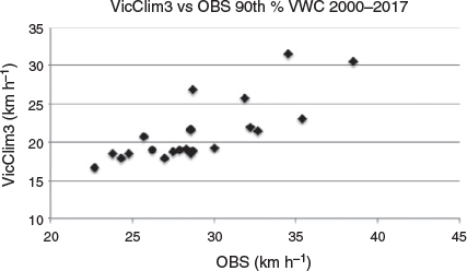
While the order of locations in Figs 3a and 3b is broadly similar, the correspondence is not perfect. Accordingly, we show the scatterplot of the two distributions in Fig. 4. There is a strong relationship between the two series, although there is some scatter around the line of best fit. A contributor to the bias and scatter may also be that while wind speed is bias corrected in the VicClim3 data set, wind direction is not.
|
The 22-location average monthly and hourly frequency distributions of annual 90th percentile VWC for VicClim3 and for OBS are shown in Fig. 5. The mean distributions by month agree very well, with a rise leading into spring, a maximum through summer and a decline through autumn and into a winter minimum. The distributions are skewed, with a greater number of springtime than autumn events. The average number of events in the peak (summer) season is around five, equivalent to approximately one every six days, and so it is still of the order of the weekly synoptic cycle, although in winter it is much lower. The diurnal distributions each show a maximum in the late afternoon/early evening. However, the OBS distribution has an earlier rise and an earlier maximum compared to the VicClim3 distribution, with the VicClim3 distribution peaking around an hour later than the OBS distribution. Reasons for this are yet unidentified, but the difference is unlikely to be significant to the later results of this paper.

|
These analyses suggest that the VicClim3 gridded data well represents regional, seasonal and diurnal variations in wind change frequency and strength across Victoria.
3.3 FFDI
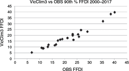
Analyses equivalent to Figs 3–5 but for the annual 90th percentiles of highest daily FFDI are shown in Figs 6–8. Ordering locations by magnitude (Fig. 6) shows the highest values in the Loddon Mallee, the Hume, the western part of Port Phillip, and the western parts of the Grampians and Barwon South West regions. Lowest values are in the elevated regions and Gippsland. The scatterplot of VicClim3 versus OBS values (Fig. 7) shows an extraordinarily strong relationship, indicating that the VicClim3 data set well represents the regional variation of annual 90th percentile FFDI, and that the bias correction described in Brown et al. (2016) has been successful.

|
|

|
Fig. 8 shows the monthly and diurnal frequency distributions of the annual 90th percentile highest daily FFDI occurrences. As shown in Harris et al. (2019), there is a strong peak in the summer and in the mid–late afternoon in each of the VicClim3 and the OBS distributions and a very close correspondence between the frequencies in the two data sets.
3.4 Joint 90th percentile event frequency
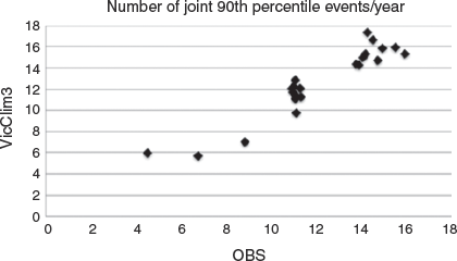
Notable features of the diurnal and seasonal frequency distributions of the VWC and the FFDI (Figs 5 and 8) is the intriguing correspondence between the time of year during which stronger wind changes are more likely (the warmer months) and the time of year when FFDI was strongest, as well as the times of day (late afternoon) when FFDI is strongest and when the strongest VWC occurs (early evening). These features led to the intriguing question of how often these events occur on the same day, as this is the situation where high adverse impact wildfire events occur. Fig. 9 shows the scatter plot of number of days per year for the 22 station locations when the annual 90th percentiles of highest daily FFDI and VWC each exceeded the VicClim3 and the OBS data sets.
|
There are two points to be made from Fig. 9. First, the relationship between the two data sets is striking, further demonstrating that the VicClim3 data set well represents the FFDI and the VWC climatologies and their variation across Victoria, and that a climatology over the full 46-year period of VicClim3 is realistic.
Second, there are three distinct clusters of points in the scatter plot of Fig. 9: one at the high end of the scale, one in the upper middle and a low frequency tail. The high-end stations are all south of the ranges but extend from Hamilton in the Barwon South West through Port Philip to Orbost in eastern Gippsland region. The locations in the middle cluster of locations are generally those in the Loddon Mallee region but with some (Kilmore Gap, Gelantipy) in elevated locations. The stations comprising the low-frequency tail are Falls Creek, Eildon and Wangaratta.
3.5 VicClim3 and AWS frequency comparison
The purpose of Section 3 is to demonstrate that the VicClim3 data set can resolve the diurnal, seasonal and geographic variations of VWC frequency, FFDI frequency and joint event frequencies. The 90th percentile of annual highest daily VWC and FFDI were selected for these comparisons. The VicClim3 data and the OBS data were closely related in terms of station location 90th percentile magnitudes for both FFDI and for VWC. Further, the frequencies of days when both the annual 90th percentiles of FFDI and VWC were exceeded were also strongly related across the 22-station sample. Accordingly, we have considerable confidence that the VicClim3 data set can be used to display the regional variation in strength of highest daily VWC and frequencies when both FFDI and VWC exceed their 90th percentile values.
4 VicClim3 46-year climatology: 1972–2017
4.1 Individual VWC and FFDI event frequency
In this section, we present two sets of climatological fields for each of the VWC and the FFDI. In the first climatological field, the spatial variation of 90th percentile of VWC and of FFDI for each season based on the VicClim3 data set for the full data set period (1972–2017) is presented in Figs 10a–d and 11a–d. This spatial variation of the seasonal 90th percentile value demonstrates where wind changes or fire danger index values are likely to be strongest across the state in each season. While this choice means that there are the same number of events at each gridpoint, the percentile values were substantially lower in some seasons (Figs 5, 8) or locations (Figs 3, 6) than others, and it may be argued that some of these lower 90th percentile values of VWC or FFDI may have limited relevance to operational decision-making.

|

|
Accordingly, a complementary threshold of how often the highest daily VWC or FFDI exceeds a fixed value across the state is likely informative. For FFDI we chose 25 as a fixed threshold: the lower limit of the very high fire danger rating. While the relevance of such a threshold will vary dramatically, say between regions such as the Mallee and East Gippsland, such variation is implicit in the 90th percentile thresholds, with the fixed threshold providing an alternative perspective. There is no such rating system for VWC strength. However, we note that the second highest quartile of values of annual 90th percentile FFDI for VicClim3 is between 20 and 25 (Fig. 6). In Fig. 3, the second highest quartile of annual 90th percentile VWC averages around 22, with only slow variation. We therefore chose to use this value of 22 to represent a fixed threshold for a threatening wind change, as it gives a frequency of occurrence comparable to that of FFDI >25 and is in the upper, but not the extreme, end of the VWC range shown in Fig. 3. It is acknowledged that this choice is arbitrary, but it will be demonstrated to provide some useful insights. The value of VWC = 22 results, for example, from a 45° wind change with speeds before and after of 17 km h−1 and for a 90° wind change with a speed before and after of 15 km h−1. These spatial distributions across Victoria, again by season, are shown in Figs 10e–f and 11e–f.
In winter (June, July, August (JJA)) the 90th percentile values of VWC (Fig. 10a) and the number of VWC > 22 events (Fig. 10e) are the lowest of the four seasons, with the highest values along the crest of the Victorian Alps east of Melbourne. These higher values are likely associated with topographically enhanced windflows.
In spring (September, October, November (SON)) there is a general increase in 90th percentile VWC values (Fig. 10b), and in the number of VWC > 22 (Fig. 10f) events. The crest of the Divide again shows a maximum, but there is an increase in numbers in the grassy plains west of Melbourne and in Gippsland.
The highest values of 90th percentile VWC (Fig. 10c) and of numbers of VWC > 22 (Fig. 10g) occur in summer (December, January, February (DJF)) with the greatest numbers in the western half of the state, decreasing slightly to the northwest. The Otway Ranges and the far southwest of the Barwon South West region show some lesser numbers than their surrounds. The eastern part of the state shows relative maxima over the high elevations in the eastern half of Victoria and in west and central Gippsland. A complex range of drivers likely contribute to these distributions, including mountain wave activity along the crest of the Great Dividing Range (the Great Divide) and downslope wind effects south of the Central Highlands and in central Gippsland. Land–sea thermal contrast is likely to have an influence along the coast west of Port Phillip and the Gippsland coast, but other factors may also have contributed. Relative minima occur near the boundary between the Port Phillip and the Gippsland regions, in the far east of the Gippsland region and in the northeast of the state where the Great Divide blocks shallow cool changes.
In autumn (March, April, May (MAM)), numbers of 90th percentile VWC events (Fig. 10d) and numbers of VWC > 22 events (Fig. 10h) decline, but less dramatically, in the grassy plains west of Melbourne, extending almost to the South Australian border, and in Gippsland compared to other regions. The values are generally lower in this autumn ‘shoulder’ season than in spring in the northwest of the state and comparable or slightly higher during the remainder of the year.
Equivalent displays for FFDI are shown in Fig. 11. In winter (JJA) the 90th percentile values are low, and the number of very high FFDI (>25) days essentially zero over the state (Fig. 11a, d). These values increase rapidly with the onset of spring (SON, Fig. 11b, f), particularly in the northwest of Victoria. Summer (DJF) has the highest numbers (Fig. 11c, g) of the seasons, with values again generally highest in the northwest and lowest in the elevated east, in eastern Gippsland, the Otway Ranges and in a narrow coastal strip west of the Otways. Both 90th percentile values and numbers of events with FFDI > 25 decline rapidly in autumn (MAM) (Fig. 11h), with highest numbers in the northwest. In this case, the autumn values are lower than the spring values, suggesting a faster buildup to the summer fire season and a more rapid decline.
4.2 Joint FFDI and VWC event frequency
This analysis of joint frequency of occurrence of days per season with both elevated fire danger and strong wind change is based on two sets of thresholds. The first uses the annual 90th percentile of FFDI and VWC at each gridpoint, and thus each gridpoint has a unique pair of threshold criteria that vary across Victoria according to the varying climatologies of VWC and FFDI (see Figs 10a–d, 11a–d). These percentiles are used rather than the seasonal percentiles from Figs 10 and 11 to avoid, for example, flagging days in winter when the FFDI was very low, yet still above the 90th percentile for the winter season. This approach better resolves the seasonal cycle. The second set of seasonal frequencies shows how often both FFDI and VWC exceed their respective fixed thresholds of 25 and 22.
The frequencies by season of joint 90th percentile events – days on which the highest FFDI and the highest VWC each exceed their 90th percentile value of annual VWC/FFDI – are presented in Fig. 12a–d, and the seasonal frequencies with which joint events exceed the defined fixed thresholds of VWC = 22 and FFDI = 25 are shown in Fig. 12e–h. As might be expected from the seasonal distributions in Figs 5 and 8, the joint frequencies are largest in summer (DJF) and lowest in winter (JJA) and are modulated spatially by the geographic distributions of FFDI and VWC, shown in Figs 10 and 11.

|
In winter (JJA), the numbers of joint events (Fig. 12a, d) are very low, largely due to the low numbers of FFDI days greater than either the annual 90th percentile or the fixed threshold.
In spring (SON) there is an increase to around 1–6 joint 90th percentile events/season across the state, apart from the higher elevations along the Great Divide, with the highest values in east Gippsland and the northwest. There are lower frequencies in the Barwon South West and the Hume regions (Fig. 12b). Joint fixed threshold (VWC > 22 and FFDI > 25, Fig. 12f) events are concentrated in the northern part of the Loddon Mallee, with highest frequencies around 4–5 per season, driven largely by the increasing numbers of FFDI > 25 events there in spring.
In summer (DJF), the highest numbers of joint 90th percentile events (Fig. 12c) are in the Barwon South West, with some 10 events per season (roughly one every nine days) and western Port Phillip regions. This broad maximum extends north through the eastern parts of the Grampians region and into the eastern part of the Loddon Mallee. There is also a maximum in Gippsland, with peak values above nine events per summer. Lowest frequencies are in the Hume region and at higher elevations. The frequency of joint fixed threshold events (Fig. 12g) is generally highest in the west of the state, apart from the higher elevations and a coastal strip. The highest numbers south of the Great Divide (driven by higher VWC frequencies) are in the Barwon South West and western Port Phillip regions with a secondary maximum in central Gippsland, whereas the higher numbers were in the Grampians and Loddon Mallee regions, driven by the higher FFDI frequencies in those regions.
In autumn (MAM), there is a marked decrease in numbers, with the highest joint 90th percentile frequencies (3–5 events per season) west of Melbourne extending to the coast and in the western part of the Gippsland region (Fig. 12d). These frequencies declined northwards across almost the entire state in autumn. The frequency of joint fixed threshold events was quite low (Fig. 12h), reflecting the rapid decrease in both numbers of FFDI > 25 days of VWC > 22 days in this season. The greatest numbers of these events, albeit only 2–3 events per season, are focussed through the grassy plains west of Melbourne.
4.3 Characteristics of strong wind changes
The spatial distributions of frequency of VWC and FFDI exceeding thresholds in Figs 10–12 do not discriminate the way in which the higher values of VWC are generated, be it backing, straight line, or veering changes, with combinations of speed increase, decrease, or relatively small changes in speed. Such analyses for each of the 22 AWS locations in Fig. 1 for the period 1972–2017 was undertaken.
A ‘straight’ wind change was defined, following Hart and Mills (2019), to be a direction change between ± 30°, a backing change between –30° and –180° difference and a veering change between 30° and 180° difference. A ‘steady’ change was defined to be ± 5 km h−1 and a speed increase and a speed decrease change defined as greater than 5 km h−1 and less than –5 km h−1 speed change respectively.
Based on the full 46-year VicClim3 data set for those 22 locations, for VWC thresholds of the annual 90th percentile value, the fixed VWC threshold of 22, and cases when the joint 90th percentiles or fixed thresholds of VWC (22) and FFDI (25) were each exceeded, numbers of events per season were calculated for each of the 22 locations. Distributions of change types and locations were broadly similar for the fixed and the 90th percentile thresholds, and here, only the results for the 90th percentile thresholds are presented.
Fig. 13 shows the distribution of direction (Fig. 13a) and speed (Fig. 13b) changes exceeding the 90th percentile VWC at each location and the same distributions for events when both VWC and FFDI exceeded their 90th percentile values. For most locations, backing wind changes predominate (Fig. 13a), suggesting frontal changes are likely the dominant change type, although the non-frontal change in the morning at Morwell (Fig. 2c, f) was a backing change, so this conclusion is not universal. More subtly, the locations in the north of the state have a greater proportion of straight or veering changes. There is a more even distribution between speed increase, steady, or speed decrease changes (Fig. 12b) but with the inland locations tending to show a greater proportion of speed increase changes.

|
When VWC >90th percentile events are also stratified by FFDI >90th percentile, the numbers of events are less, but the proportion of backing changes becomes very high at essentially every location, and there is still a tendency for speed increase changes to be relatively higher at the inland locations. Thus, on days of elevated fire danger any strong wind change is likely to be a backing wind change.
5 Discussion and conclusions
In this paper, we have presented the first spatial climatology of 1-hour wind change strength over Victoria using the 46-year high spatial (4 km) resolution VicClim3 gridded data set. The strength of the wind change was defined as the magnitude of the vector difference between two successive hourly wind vectors – the VWC. While this metric has not to our knowledge been used in such a climatological study, subjective assessments and comparison with the WCRI metric that has had some use in the Bureau of Meteorology indicate that it does identify the types of wind change associated with significant wildfire events.
The frequency of occurrence of the 90th percentile of highest daily VWC for all days in the data set showed a strong seasonal cycle, with the frequencies, on average, some four times larger in summer than in winter. There is also a clear diurnal signal, with the greatest frequencies in the late afternoon and early evening. As these distributions are not unlike the seasonal and diurnal frequency distributions of FFDI, the occurrence of high values of both VWC and FFDI occurring on the same day were analysed spatially by season.
The spatial distribution of the strength of strong wind changes over Victoria for the full 1972–2017 VicClim3 data set was presented using two threshold values of VWC: the magnitude of the 90th percentile of annual highest daily VWC and a selected fixed threshold of 22. Percentile and fixed threshold values are generally highest in the south and west of the state and in summer. There are generally maxima across the highest elevations associated with topographically induced flows, particularly in the cooler months. Lowest values are seen in the Hume region.
When joint thresholds are tested, summer is the major season for joint VWC and FFDI events. Joint 90th percentile events are most frequent in summer in the western part of the state between the Great Divide and the Otway Ranges. It is likely that many of these events were driven by the dry cool changes that are preceded by hot, dry, northerly winds (high FFDI) and are often followed by gusty winds (Reeder 1986; Mills 2002; Engel et al. 2013). It is perhaps not coincidental that the disastrous fire events cited in the Introduction occurred in these areas. Fixed threshold joint events are also at their maximum in this region in summer, although the increasing frequencies of very high FFDI days in the northwest lead to this region also having increased numbers of these joint events.
There are secondary maxima in each joint frequency type near and inland from the Gippsland Lakes. The lowest values are seen in eastern Gippsland, the alpine zone, and the Hume region. However, on a given day, wind changes in these regions can still affect fires dramatically. There are relatively less studies of wind changes in these regions than in the west of the state, although Mills (2005) presented an example of a strong dry frontal change on the Gippsland coast on 30 January 2003 when fires were active in the alpine areas north of Gippsland, and Buckley (1992) described a fire near Bemm River in East Gippsland on 14 October 1988 that was affected both by strong prefrontal winds and a late afternoon backing wind change. The highest VWCs at Bairnsdale and Orbost on that day were ranked at the 96th and 93rd percentiles respectively. An example in the Hume region is the Beechworth-Mudgegonga fire on ‘Black Saturday’ 2009 (Teague et al. 2010; Engel et al. 2013). The VWC at Wangaratta on that evening was 28 in the VicClim3 data set, which was in the highest 2% of values at Wangaratta in the 46 years of the data set.
In spring, the frequency of joint events increases first in the northwest, associated with both the rapid increase in the FFDI values there in that season and with an increase in VWC values there. In autumn, the joint frequency values decreases substantially, but there is a relative maximum in frequency west of Melbourne through to the South Australian border associated with a relative maximum in VWC.
The frequency of joint events is not necessarily random. Both the FFDI and the VWC are higher with higher wind speeds, and so there is some positive relation between the two. There is also the synoptic control, with, as discussed above, both elevated FFDI and elevated wind change strength associated with the passage of dry cold fronts. There may be other links too, and this is an intriguing avenue for further research.
The two pairs of thresholds were chosen somewhat arbitrarily for this initial study and each has its limitations, with the 90th percentile thresholds having values that are perhaps too low in some areas or seasons for practical relevance for fire weather planning. The fixed thresholds, particularly for FFDI, have different relevance to fire management depending on vegetation type and load. Accordingly, for future applications it may be worthwhile developing thresholds for individual regions based on operational experience in those regions or by matching observed fire outcomes (e.g. area burned) with the VWC and FFDI on the day. The thresholds used also tended to focus on the summertime when bushfires are most prevalent, but similar analyses with thresholds appropriate to shoulder seasons and prescribed burning guidelines may better inform those operations.
The analysis of wind direction and speed changes associated with wind changes exceeding the thresholds show that a large proportion of strong changes are associated with backing winds and that winds increase more frequently across the 1-hour change period at inland locations than at others. These speed changes may not reflect changes over longer periods that will affect fire management (e.g. a speed increase some hours after an initial direction change with speed decrease), but this analysis does provide a basis for future work. Intriguing avenues for investigation would include the documentation of any regional variations in dominant wind directions before and after backing versus veering wind changes as well as regional and seasonal variations of times of strong wind changes.
Neither the interannual variability of frequency of strong wind changes nor any long-term trends in strong wind change frequency have been addressed in this paper. There would be clear academic, and likely practical, interest in the interannual variability together with the relationship of any such variability of known drivers of the Australian climate (e.g. Harris and Lucas 2019). Any such relationships would have application for seasonal planning, while any trends with time could impact longer term planning.
Conflicts of interest
The authors declare that they have no conflicts of interest.
Acknowledgements
The Victorian Department of Environment, Land, Water, and Planning and the Bushfire and Natural Hazards Cooperative Research Centre funded and managed the development of the VicClim3 data set respectively. Dr Musa Kilinc (Country Fire Authority, Victoria) and Dr Paul Fox-Hughes (Bureau of Meteorology) reviewed an early version of this paper. The positive and constructive comments by the three anonymous reviewers are appreciated by the authors and led to numerous improvements to the original manuscript. This research did not receive any specific funding.
References
Badlan, R. L., Lane, T. P., Mills, G. A., and Caine, S. (2012). Mesoscale modeling of two ‘drying events’: governing processes and implications for fire danger. Aust. Meteor. Oceanog. J. 62, 143–156.| Mesoscale modeling of two ‘drying events’: governing processes and implications for fire danger.Crossref | GoogleScholarGoogle Scholar |
Berson, F. A., Reid, D. G. and Troup, A. J. (1957). The summer cool change of southeastern Australia. I: General behaviour. Technical Paper No. 8. (CSIRO Division of Meteorological Physics: Mordialloc, Australia). 48pp.
Berson, F. A., Reid, D. G. and Troup, A. J. (1959). The summer cool change of southeastern Australia. II. Effects of differential heating and modification of advective change. Technical Paper No. 9. (CSIRO Division of Meteorological Physics: Mordialloc, Australia). 69 pp.
Bianco, L., Djalalova, I. V., Wilczak, J. M., Cline, J., Calvert, S., Konopleva-Akish, E., Finley, C., and Freedman, J. (2016). A wind energy ramp tool and metric for measuring the skill of numerical weather prediction models. Wea. Forecasting 31, 1157–1177.
| A wind energy ramp tool and metric for measuring the skill of numerical weather prediction models.Crossref | GoogleScholarGoogle Scholar |
Bond, N. A., Mass, C. F., and Overland, J. E. (1996). Coastally trapped wind reversals along the United States west coast during the warm season. Part 1: Climatology and temporal evolution. Mon Wea. Rev. 124, 430–445.
| Coastally trapped wind reversals along the United States west coast during the warm season. Part 1: Climatology and temporal evolution.Crossref | GoogleScholarGoogle Scholar |
Brown, T., Mills, G., Harris, S., Podnar, D., Reinbold, H., and Fearon, M. (2016). A bias corrected WRF mesoscale fire weather dataset for Victoria, Australia 1972-2012. J. South. Hemisph. Earth Syst. Sci. 66, 281–313.
| A bias corrected WRF mesoscale fire weather dataset for Victoria, Australia 1972-2012.Crossref | GoogleScholarGoogle Scholar |
Buckley, A. J. (1992). Fire behaviour and fuel reduction burning: Bemm River wildfire, October 1988. Australian Forestry 55, 135–147.
| Fire behaviour and fuel reduction burning: Bemm River wildfire, October 1988.Crossref | GoogleScholarGoogle Scholar |
Bureau of Meteorology (1984). Report on the meteorological aspects of the Ash Wednesday fires – 16 February 1983. (Bureau of Meteorology: Melbourne Australia). 143 pp.
Bureau of Meteorology (2014). Hazardous Weather Phenomena. Wind Shear. Available at www.bom.gov.au/aviation/knowledge-centre/. [Accessed 7 June 2010].
Case, J. L., Manobianco, J., Lane, J. E., Immer, C. D., and Merceret, F. J. (2004). An objective technique for verifying sea breezes in high-resolution numerical weather prediction models. Wea. Forecasting 19, 690–705.
| An objective technique for verifying sea breezes in high-resolution numerical weather prediction models.Crossref | GoogleScholarGoogle Scholar |
Cheney, P., Gould, J., and McCaw, L. (2001). The dead-man zone — A neglected area of fire fighter safety. Aust. For. 64, 45–50.
| The dead-man zone — A neglected area of fire fighter safety.Crossref | GoogleScholarGoogle Scholar |
Clarke, R. H. (1955). Some observations and comment on the sea breeze. Aust. Meteor. Mag. 11, 47–68.
Clarke, R. H. (1983). Fair weather nocturnal inland wind surges and atmospheric bores: Part 1 Nocturnal wind surges. Aust. Meteor. Mag. 31, 133–145.
Clarke, H., Evans, J. P., and Pitman, A. J. (2013). Fire weather simulation skill by the Weather Research and Forecasting (WRF) model over south-east Australia from 1985 to 2009. Int. J. Wildland Fire 22, 739–756.
| Fire weather simulation skill by the Weather Research and Forecasting (WRF) model over south-east Australia from 1985 to 2009.Crossref | GoogleScholarGoogle Scholar |
Colle, B. A., Mass, C. F., and Ovens, D. (2001). Evaluation of the timing and strength of MM5 and Eta surface trough passages over the eastern Pacific. Wea. Forecasting 16, 553–572.
| Evaluation of the timing and strength of MM5 and Eta surface trough passages over the eastern Pacific.Crossref | GoogleScholarGoogle Scholar |
Country Fire Authority (1999). Reducing the risk of wildfire entrapment. A case study of the Linton Fire. Country Fire Authority Report. (Country Fire Authority: Burwood East, Vic). 16 pp.
Cruz, M. G., Sullivan, A. L., Gould, J. S., Sims, N. C., Bannister, A. J., Hollis, J. J., and Hurley, R. J. (2012). Anatomy of a catastrophic wildfire: The Black Saturday Kilmore East fire in Victoria, Australia. Forest Ecol. Manag. 284, 269–285.
| Anatomy of a catastrophic wildfire: The Black Saturday Kilmore East fire in Victoria, Australia.Crossref | GoogleScholarGoogle Scholar |
Engel, C., Lane, T. P., Reeder, M. J., and Rezny, M. (2013). The meteorology of Black Saturday. Quart. J. Roy. Meteor. Soc 139, 585–589.
| The meteorology of Black Saturday.Crossref | GoogleScholarGoogle Scholar |
Fox-Hughes, P., Harris, R., Lee, G., Grose, M., and Bindoff, N. (2014). Future fire danger climatology for Tasmania, Australia, using a dynamically downscaled regional climate model. Int. J. Wildland Fire 23, 309–321.
| Future fire danger climatology for Tasmania, Australia, using a dynamically downscaled regional climate model.Crossref | GoogleScholarGoogle Scholar |
Garratt, J. R. (1986). Boundary layer effects on cold fronts at a coastline. Bound. Lay. Met. 36, 101–5.
| Boundary layer effects on cold fronts at a coastline.Crossref | GoogleScholarGoogle Scholar |
Garratt, J. R. (1988). Summertime fronts in southeast Australia - Behaviour and low-level structure of main frontal types. Mon. Wea. Rev. 116, 636–649.
| Summertime fronts in southeast Australia - Behaviour and low-level structure of main frontal types.Crossref | GoogleScholarGoogle Scholar |
Garratt, J. R., and Physick, W. L. (1986). Numerical study of atmospheric gravity currents. Part I: Simulations and observations of cold gravity currents. Beitr. Phys. Atmos. 59, 282–300.
Garratt, J. R., and Physick, W. L. (1987). Numerical study of atmospheric gravity currents. Part I: Simulations and observations of cold gravity currents. Beitr. Phys. Atmos. 60, 88–102.
Harris, S., Mills, G., and Brown, T. (2017). Variability and drivers of extreme fire weather in fire-prone areas of southeastern Australia. Int. J. Wildland Fire 26, 177–190.
| Variability and drivers of extreme fire weather in fire-prone areas of southeastern Australia.Crossref | GoogleScholarGoogle Scholar |
Harris, S., and Lucas, C. (2019). Understanding the variability of Australian fire weather between 1973 and 2017. PLoS ONE 14, e0222328.
| Understanding the variability of Australian fire weather between 1973 and 2017.Crossref | GoogleScholarGoogle Scholar | 31536523PubMed |
Harris, S., Mills, G., and Brown, T. (2019). Victorian fire weather trends and variability. In ‘23rd International Congress on Modelling and Simulation, Canberra, ACT, Australia’. Available at https://modsim2019.exordo.com/programme/presentation/590 [Accessed 6 September 2020]
Hart, T., and Mills, G. A. (2019). Abrupt wind speed changes on northern Port Phillip. Bulletin of the Australian Meteorological and Oceanographic Society 32, 10–15.
Huang, X., and Mills, G. (2006a). Objective identification of wind change timing from single station observations. Part 1: Methodology and comparison with subjective wind change timings. Aust. Meteor. Mag. 55, 261–274.
Huang, X., and Mills, G. (2006b). Objective identification of wind change timing from single station observations. Part 2: Towards the concept of a wind change climatology. Aust. Meteor. Mag. 55, 275–288.
Johnson, R. H., Schumacher, R. S., and Ruppert, J. H. (2014). The role of convective outflow in the Waldo Canyon fire. Mon. Wea. Rev. 142, 3061–3080.
| The role of convective outflow in the Waldo Canyon fire.Crossref | GoogleScholarGoogle Scholar |
Kepert, J., Tory, K., Thurston, W., Ching, S., Fawcett, R., and Yeo, C. (2016). Fire escalation by downslope winds. Hazard Note 24, Bushfire and Natural Hazards Cooperative Research Centre. Available at https://www.bnhcrc.com.au/hazardnotes/24 [Accessed 15 September 2020]
Lahaye, S., Sharples, J., Matthews, S., Heemstra, S., Price, O., and Badlan, R. (2018). How do weather and terrain contribute to firefighter entrapments in Australia? Int. J. Wildland Fire 27, 85–98.
| How do weather and terrain contribute to firefighter entrapments in Australia?Crossref | GoogleScholarGoogle Scholar |
Loewe, F. (1945). Frontal hours at Melbourne. R.A.A.F. Weather Research and Development Bulletin 3, 13–19.
Ma, Y., Huang, X., Mills, G. A., and Parkyn, K. (2010). Verification of mesoscale NWP forecasts of abrupt cold frontal wind changes. Wea. Forecasting 25, 93–112.
| Verification of mesoscale NWP forecasts of abrupt cold frontal wind changes.Crossref | GoogleScholarGoogle Scholar |
McArthur, A. G., Cheney, N. P., and Barber, J. (1977). The fires of 12 February 1977 in the western district of Victoria. Joint report by CSIRO Division of Forest Research, Canberra and the Country Fire Authority. (CSIRO Division of Forest Research: Canberra, ACT). 73pp
Mills, G. A. (2002). A case of coastal interaction with a cool change. Aust. Meteor. Mag. 51, 203–221.
Mills, G. A. (2005). On the sub-synoptic scale meteorology of two extreme fire weather days during the Eastern Australian fires of January 2003. Aust. Meteor. Mag. 54, 265–290.
Mills, G. A., and Pendlebury, S. (2003). Processes leading to a severe wind-shear incident at Hobart Airport. Aust. Meteor. Mag. 52, 171–188.
Mills, G. A., and Morgan, E. (2006). The Winchelsea Convergence – using radar and mesoscale NWP to diagnose cool change structure. Aust. Meteor. Mag. 55, 47–58.
Muir, L., and Reeder, M. J. (2010). Idealised modeling of land falling cold fronts. Quart. J. Roy. Meteor. Soc. 136, 2147–2161.
| Idealised modeling of land falling cold fronts.Crossref | GoogleScholarGoogle Scholar |
Page, W. G., Freeborn, P. H., Butler, B. W., and Jolly, W. M. (2019). A review of US wildland firefighter entrapments: trends, important environmental factors and research needs. Int. J. Wildland Fire 28, 551–569.
| A review of US wildland firefighter entrapments: trends, important environmental factors and research needs.Crossref | GoogleScholarGoogle Scholar |
Peace, M., McCaw, L., Kepert, J., Mills, G., and Mattner, T. (2015a). WRF and SFIRE simulations of the Layman fuel reduction burn. Aust. Meteor. Oceanog. J. 65, 302–317.
| WRF and SFIRE simulations of the Layman fuel reduction burn.Crossref | GoogleScholarGoogle Scholar |
Peace, M., Mills, G., Mattner, T., McCaw, L., and Kepert, J. (2015b). Fire-modified meteorology in a coupled fire-atmosphere model. J. Appl. Meteorol. Climatol. 54, 704–720.
| Fire-modified meteorology in a coupled fire-atmosphere model.Crossref | GoogleScholarGoogle Scholar |
Physick, W. L. (1988). Mesoscale modelling of a cold front and its interaction with a diurnally heated land mass. J. Atmos. Sci. 45, 3169–87.
| Mesoscale modelling of a cold front and its interaction with a diurnally heated land mass.Crossref | GoogleScholarGoogle Scholar |
Reeder, M. J. (1986). The interaction of a surface cold front with a prefrontal thermodynamically well-mixed boundary layer. Aust. Meteor. Mag. 34, 137–148.
Reeder, M. J., and Smith, R. K. (1987). A study of frontal dynamics with application to the Australian summertime cool change. J. Atmos. Sci. 44, 687–705.
| A study of frontal dynamics with application to the Australian summertime cool change.Crossref | GoogleScholarGoogle Scholar |
Reeder, M. J., and Smith, R. K. (1998). Mesoscale Meteorology. In ‘Meteorology of the Southern Hemisphere’. (Eds D. Vincent and D. J. Karoly.) pp. 201–242. (American Meteorological Society: Boston, USA). 420pp.
Reeder, M. J., and Tory, K. J. (2005). The effects of the continental boundary layer on the dynamics of fronts in a 2D model of baroclinic instability. II: Surface heating and cooling. Quart. J. Roy. Meteor. Soc. 131, 2409–2429.
| The effects of the continental boundary layer on the dynamics of fronts in a 2D model of baroclinic instability. II: Surface heating and cooling.Crossref | GoogleScholarGoogle Scholar |
Reid, D. (1957). Evening wind surges in South Australia. Aust. Meteor. Mag. 16, 23–32.
Rife, D. L., and Davis, C. A. (2005). Verification of temporal variations in mesoscale numerical wind forecasts. Mon. Wea. Rev. 133, 3368–3381.
| Verification of temporal variations in mesoscale numerical wind forecasts.Crossref | GoogleScholarGoogle Scholar |
Sharples, J. J., McRae, R. H. D., Mills, G. A., and Weber, R. O. (2010). Foehn-like winds and elevated fire danger conditions in southeastern Australia. J. Appl. Meteorol. Climatol. 49, 1067–1095.
| Foehn-like winds and elevated fire danger conditions in southeastern Australia.Crossref | GoogleScholarGoogle Scholar |
Smith, R. K., and Reeder, M. J. (1988). On the movement and low level structure of cold fronts. Mon. Wea. Rev. 116, 1927–1944.
| On the movement and low level structure of cold fronts.Crossref | GoogleScholarGoogle Scholar |
Teague, B., McLeod, R., and Pascoe S. (2010). 2009 Victorian Bushfires Royal Commission. Final report. Parliament of Victoria, Melbourne.
Tory, K. J., and Reeder, M. J. (2005). The effects of the continental boundary layer on the dynamics of fronts in a 2D model of baroclinic instability. I: An insulated lower surface. Quart. J. Roy. Meteor. Soc. 131, 2389–2408.
| The effects of the continental boundary layer on the dynamics of fronts in a 2D model of baroclinic instability. I: An insulated lower surface.Crossref | GoogleScholarGoogle Scholar |
Yarnell Hill Fire Investigation Report Team (2013). Yarnell Hill Fire: June 30, 2013. Serious Accident Investigation Report. (Arizona State Forestry Division, Office of the State Forester: Phoenix, AZ, USA). Available at https://www.documentcloud.org/documents/800042-yarnell-hill-serious-accident-investigation-report.html [Accessed 8 April 2020]