
Verification of moist surface variables over northern Australia in a high-resolution reanalysis (BARRA)
Peter T. May A D , Blair Trewin B , Chun-Hsu Su B and Bertram Ostendorf C
A School of Earth Atmosphere and Environment, Monash University, Clayton, Australia.
B Bureau of Meteorology, Melbourne, Australia.
C University of Adelaide, Adelaide, Australia.
D Corresponding author. Email: peter.may@monash.edu
Journal of Southern Hemisphere Earth Systems Science 71(2) 194-202 https://doi.org/10.1071/ES21007
Submitted: 13 April 2021 Accepted: 6 August 2021 Published: 20 September 2021
Journal Compilation © BoM 2021 Open Access CC BY-NC-ND
Abstract
Reanalyses are important tools for understanding past weather and climate variability, but detailed verification of near surface humidity variables have not been published. This is particularly concerning in tropical regions where humid conditions impact meteorology and human activities. In this study, we used screen level temperature and humidity data from a high-resolution atmospheric regional reanalysis, the Bureau of Meteorology Atmospheric high-resolution Regional Reanalysis for Australia (BARRA), validated against automatic weather stations (AWS) data for 32 sites across northern Australia. Overall, the BARRA data was reliable, with the time series from the AWS and BARRA being very highly correlated, but there were some seasonal and diurnally varying biases. The variability of the differences also changed from location to location and as a function of time of day and season, but much less than the biases. This variability was less than the ‘weather signal’ as evidenced by the high correlations. In particular, the amplitude of the diurnal cycle was overestimated, particularly in the dry (winter) season. In general, the differences in temperature were larger than those of the dew point temperature, and the wet bulb temperature had the least uncertainty. Overall, this study contributes to a better understanding of the effectiveness of reanalyses for examining the impact of moist variables on tropical climate variability.
Keywords: BARRA, BARRA-R, high-resolution reanalysis, humidity, northern Australia, verification, wet bulb temperature.
1 Introduction
Reanalyses are key tools in understanding past weather and climate trends over recent decades to a century. These have been used on global scales at modest spatial resolution (e.g. ~30–70 km) and at higher resolution on regional scales (~2–12 km). As expected, these reanalyses have been extensively verified against observational data, including surface and tower measurements of temperature and rainfall (e.g. Bosilovich et al. 2008; Decker et al. 2012; Su et al. 2019) as well as soundings (e.g. Jakobson et al. 2012). Other analyses have focussed on particular regions (e.g. Szczypta et al. 2011; Jakobson et al. 2012). Less attention has been paid to moist thermodynamic variables, such as the dew point temperature (TD) and wet bulb temperatures (TWB) near the surface, with some exceptions, such as comparison with column precipitable water (Bock et al. 2005). Nor has there been a focus on the tropics where the impact of humidity on meteorology and human activities are acute.
Given the difficulty of maintaining high quality wet bulb instrumental records (e.g. Lucas 2010), extremes of TWB and their trends are probably best explored through reanalyses. However, this requires an assessment of the accuracy of these analyses.
This study explores comparisons of hourly point surface observations with a 12-km atmospheric regional reanalysis data (Bureau of Meteorology Atmospheric high-resolution Regional Reanalysis for Australia, BARRA-R, or BARRA for brevity in this work; Su et al. 2019) at several sites in tropical northern Australia to explore this issue. Perfect agreement is not expected as local terrain and unresolved or poorly resolved local circulations may produce significant differences.
2 Data sets
Surface automatic weather station (AWS) data from the Australian Bureau of Meteorology has been collected from 32 sites in northern tropical Australia (Fig. 1, Appendix 1). These provide a wide geographic spread, with locations ranging from near coastal and peninsula sites to far inland. These sites record hourly temperature (T), relative humidity (RH) and, in some locations, TD and TWB. Where TWB was not recorded, it was calculated from the temperature and RH using the approximation of Stull (2011) given in Appendix 2. Likewise, TD was calculated from the temperature and RH where it was not recorded. The Bureau of Meteorology AWS network is well supported, but there is occasional bad humidity data where the wet bulb sensors become dry and T~TD~TWB, but this only affects ~0.004% of the data. The overlap of AWS data with the BARRA data set varies in length from less than a year to essentially the full data set with a median length of 13 years, but 13 of the sites are less than about 6 years long. There are 16 sites with records greater than 14 years.

|
The BARRA data is hourly, covers the period from January 1990 to February 2019 and has a horizontal grid spacing of around 12 km across Southeast Asia and the Maritime Continent as well as northern Australia. The data set comprises standard variables, including temperature, pressure, humidity, wind, cloud cover and rainfall. It was developed by assimilating a wide range of surface, satellite, aircraft and radiosonde observations in a coupled atmosphere–land model, namely the UK Met Office Unified Model for the atmosphere and the Joint UK Land Environment Simulator for the land (Walters et al. 2017). The model is set up with global atmosphere configurations suited for this moderate resolution and is nested within the European Centre for Medium-Range Weather Forecasts (ECMWF) Re-Analysis (ERA-Interim) global data set (Dee et al. 2011). BARRA is documented by Su et al. (2019).
Calculation of RH from the model data was performed using the approximations of Buck (1981), given in Appendix 2, for calculating saturation vapour pressure. Note this is very close to the Goff-Gratch formulation used in the modelling scheme for the warm temperatures in these regions. As with the observations, the TWB was also calculated using the method of Stull (2011).
It should be noted that the observations used in the evaluation have also been assimilated in BARRA. Although the observational data is not strictly independent from BARRA, the data is a small part of an extensive range of observational data jointly assimilated in BARRA, and a significant part (50%) of the evaluated BARRA data sits outside the analysis windows (Su et al. 2019).
Since the BARRA grid is relatively coarse compared with the point observation footprint, there is always a height discrepancy between the grid cell height and the station altitude. This can be up to several hundred metres in mountainous terrain as can be found near parts of the Australian east coast. The bias from these height offsets is corrected by assuming a dry adiabat for all the temperature variables and constant specific humidity. Note this is strictly not correct, particularly near the surface, but it is a reasonable approximation over several hundred metres, and where the height difference is small, the correction is likewise small. This correction does act to reduce the bias in all cases, so is worthwhile.
3 Overall statistics
Data from the AWS and the BARRA analysis were matched in time, and the nearest land pixel was used. Note that some sites are on peninsulas and that the BARRA grid has some sites where the nearest grid point, such as Darwin airport, is characterised as an ocean grid point. The BARRA analyses show a rapid transition between off-shore and coastal locations of the surface temperature and humidity fields in terms of the diurnal cycle of temperature and the corresponding maximum and minimum temperatures (Tmax and Tmin, respectively) as has been observed near Darwin (e.g. May et al. 2012).
Time series for each site were collected, and the bias, standard deviation, skewness and correlation of the differences in T, TWB and RH between the AWS and BARRA data over the full station data length were calculated. From these statistics we then computed the median bias and standard deviations in the distributions over all the sites for the overall statistics (Appendix 1), noting the record lengths at the various sites vary from one site as short as 6 months to the full 29 years with a median of 13 years (Appendix 1). No attempt was made to weight the results to those sites with longer records because we wanted to sample as many locations as possible, and as can be seen in Table 1, the range of values for each variable was relatively small. The skewness of the distributions were also relatively small.

|
The biases were much less than the standard deviations of the differences between the measurements. The magnitudes of the standard deviation of the temperature estimate differences were significant but generally much smaller than the daily and seasonal variations of the data, indicating that they were within a useful range for many applications. Note that the differences are at least partly due to comparing point measurements with an areal average and the corresponding lack of perfect overlap.
The correlations between the two estimates were very high for all the variables. This reflects a good mapping of the diurnal cycle and seasonal variations on both sets of time series, so high correlations are expected, but even the specific humidity shows correlations of order 0.9. Further, these high correlations mean that the covarying signal was much greater than the differences between the AWS and BARRA estimates even with the seasonal cycle removed.
The TWB differences were systematically smaller than the temperature. The dynamic range of the individual TWB time series tends to be smaller than the temperature, but notably, the variance was still less and correlations were higher despite the relative reduction in amplitude of the true variations and potential contributions from both the temperature and humidity terms.
4 Statistics of daily maxima and minima
For many applications, it is the daily maximum and minimum values that are important. In order to test BARRA for this, in Table 2, we calculated the daily maxima and minima using a daily definition of 00–23 UTC to allow for the three time zones. With the daily cycle subtracted, the standard deviation of the differences between the AWS and BARRA was reduced, and the correlations remained very high, although there was some greater variance between sites. The bias values include the median bias over all the separate sites as well as the standard deviation of these biases. The variation between sites was comparable to or larger than the overall median bias. For all sites the magnitude of the average differences between the AWS and BARRA was less than the standard deviation of the differences.

|
However, the magnitude of the temperature biases was larger for these daily values than for the hourly time series, with BARRA showing a negative bias for the minimum temperature and positive for the maximum. Thus, BARRA overestimated the amplitude of the diurnal cycle of temperature at most sites over land, with a mean bias of 1.3°C. Su et al. (2019) compared the BARRA reanalysis with a semi-independent 5-km gridded surface analysis of temperature (and rainfall), Australian Water Availability Project (Jones et al. 2009). This comparison showed that BARRA underestimated the diurnal range over much of southern Australia, but gave more structure in the relatively sparsely observed northern area. In particular, the regions where our sites were used often showed similar overestimation of the diurnal cycle (Su et al. 2019, their Fig. 5). Note that overestimation of the amplitude of diurnal temperatures has also been reported in the ECMWF reanalysis for the Mississippi river basin (Betts et al. 2008). In contrast, the TWB and TD biases were both cool (dry) and the diurnal variation only had a small bias. Note also the extremely high correlations between the two TWB time series, reflecting the model data resolving the seasonal cycle but with relatively low noise.
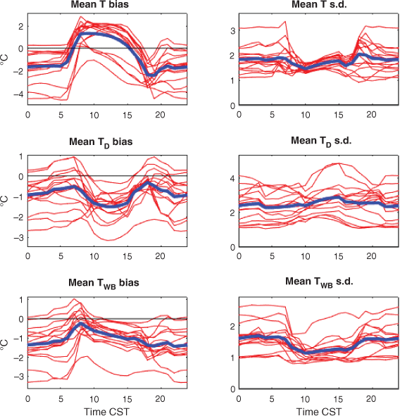
The origin of these biases could arise from a number of sources, including local circulations, biases in surface, cloud, radiation and boundary layer parameterisations and the extrapolation from model level to the screen level. For example, AWS sites separated by only a few kilometres may have marked variations in minimum temperature associated with local circulations and drainage flows (e.g. Trewin 2005). Fig. 2 shows the mean biases and standard deviations of the temperature, dew point and wet bulb as a function of local time for those (16) sites with records greater than 14 years. All the temperature biases show similar behaviour with a rapid transition to BARRA being positively biased near sunrise and a more gradual shift to negative biases at sunset. In contrast, the average standard deviations of the differences show little diurnal cycle, but there are some sites where there are significant variations. In particular, there was an outlying curve from Argyle Aerodrome, located near a large inland lake, which showed a distinct increase in the evening. The subgrid characterisation of the associated model grid cell includes this lake as inland water, but local circulations may still have an impact. Other sites showed some additional variations around sunrise and sunset, possibly arising from comparing points with areal averages. The TD shows a negative (dry) bias in BARRA at all times, but this is larger during the day, possibly indicating too much mixing. The wet bulb bias sees the individual temperature and the dew point biases essentially cancel, albeit with an underestimation by BARRA with a minimum shortly after sunrise. The standard deviations of these moist variables show relatively small variance, although the TWB differences tend to have smaller variability during the day.
|
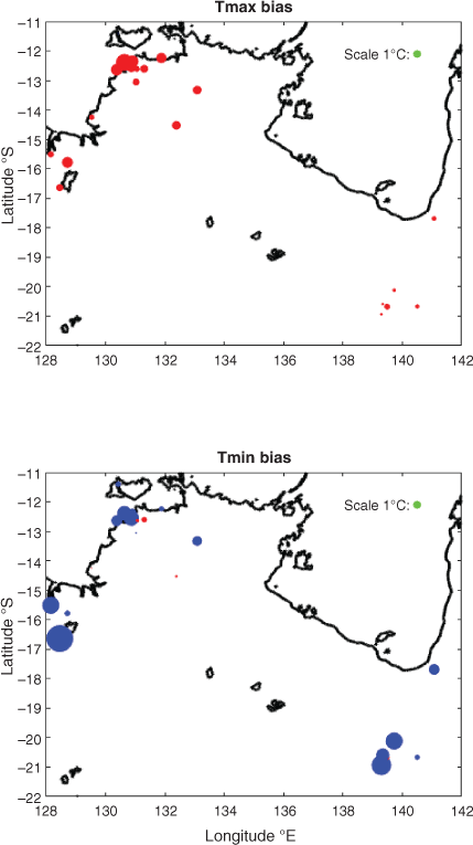
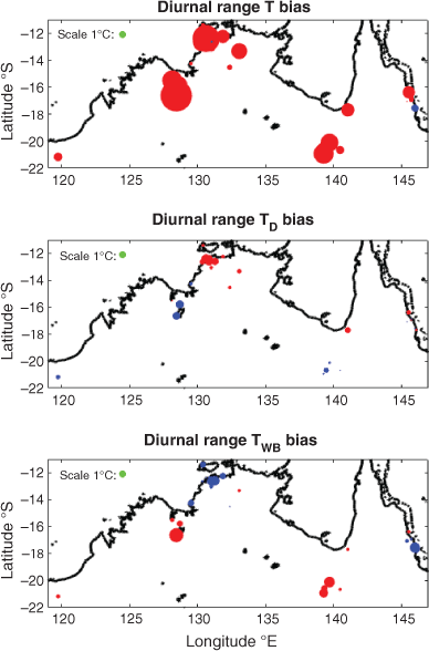
The spatial distribution of these biases could provide some insights into their causes. Some of the largest Tmax biases are near the coast, but these have nearby sites with small biases, so that the observed ocean–coastal transition of the temperature and humidity diurnal variations does not seem to be a major factor leading to errors (Fig. 3). Similar large variations in nearby sites are also seen inland. Likewise, the largest Tmin biases tend to be inland, but again there is no clear spatial patterns, with nearby sites exhibiting large variations in the bias, both near the coast and inland. Thus, there is also little evidence of systematic differences between the coastal areas and inland. This indicates that small-scale variability is important, with potentially unresolved circulations and their impacts as well as variations in land surface perhaps dominating other factors, such as radiation and the extrapolation, down to the 2 m level where biases may be expected to be more spatially uniform. The maxima and minima of TD and TWB also show small spatial scale variability and no clear signal. However, when these are combined, there is a clear north south gradient in the magnitude of the biases in the diurnal variation of the moist variables TD and TWB (Fig. 4). Although this is a large spatial scale variation, it also reflects the meridional gradient of rainfall and soil moisture.
|
|
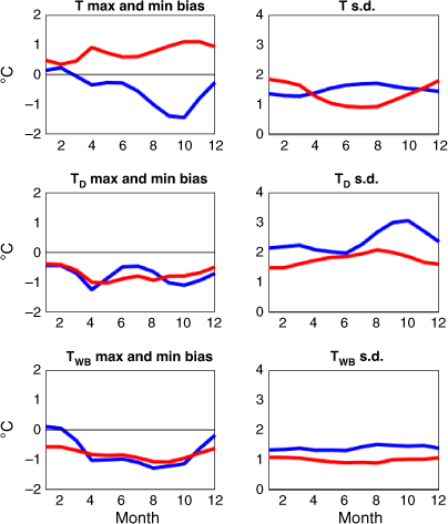
5 Seasonal variations
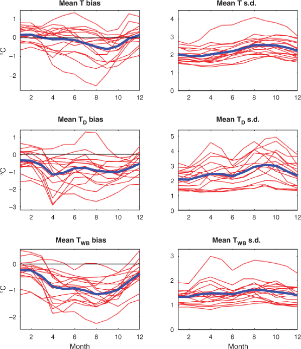
The diurnal variations of bias and potential linkages to the model boundary layer parameterisation, land surface and radiation schemes leads to the question of any systematic variations with season. Fig. 5 shows the seasonal variations for the mean bias and standard deviations of T, TD and TWB for the same 16 locations. It is clear that the seasonal variations are much smaller than the diurnal ones, but there are still clear signals. There are significant variations between the various sites for all the variables, but the temporal variations are generally consistent. The temperature bias tends to be small and negative (AWS > BARRA) in the late winter and build-up (October–December) seasons whereas the variability slightly increases. These biases are smallest in the wet season (January–March) when there is the most convection, cloud cover, etc. (e.g. May et al. 2012 and references within). The TD analyses show a dry bias in BARRA throughout the dry season (April–September), and this manifests as a consistent dry bias in the TWB. The fact that these biases are smallest in the wet season indicates that rainfall biases in BARRA (Su et al. 2019, section 3) are unlikely to be responsible for the overall dry bias. Similar to the diurnal biases, there was little consistent spatial structure evident in the sparse network when these biases were plotted on maps (not shown). There is far less seasonal variation in the standard deviations of the differences between the AWS and BARRA, although there is a weak maximum of the standard deviation of the differences in temperature and dew point in September and October, which is the end of the dry season.
|
We further expand on this by examining the biases and variation of the daily maxima and minima as a function of month (Fig. 6). The temperature panel shows a distinct cycle where the biases are relatively small in the wet season and progressively grow larger, with BARRA being greater than the AWS for Tmax and lower for Tmin. A candidate to explain this may be local flows. For example, as the amount of local convection increases in the build-up months prior to the monsoon a source of cool minimum bias is where the AWS data may be affected by storm outflows associated with thunderstorms causing local temperature changes of several degrees, which will not be resolved in the reanalysis (e.g. Keenan and Carbone 1992; May 1999). However, the nighttime cool bias starts to increase well before the storm season, and the daytime warm bias also increases from mid-year until well into the build-up season. This points to some issues in the analysis in clear sky conditions for the screen level estimates. This could be associated with model biases in radiation, land surface characteristics and boundary layer parameterisations or the extrapolation from the lowest model level to the screen level. All may contribute.
|
The moisture variable (TD), in contrast, demonstrates a weaker seasonal variation of dry bias, but there is a clear increase in variability during the pre-monsoon build-up where local circulation trigger storms. Again, moist outflows may contribute to this, but the temperature variations do not show a similar peak. These T and TD variations result in low seasonal variability of TWB.
6 Summary and conclusions
This paper compared the BARRA reanalysis temperature and humidity related screen level data with AWS data for a number of locations across northern Australia. This is particularly important for tropical regions, as the weather and its impact are affected by high humidity and measuring variables, such as TWB, are prone to instrumental issues. We have focussed on the air temperature, the TD, which is a purely humidity based variable, and the TWB, which is a combination of temperature and humidity.
In general, there was good agreement between the AWS and BARRA time series considering the comparison is between areal averages and point measurements. The model biases relative to the observations and the standard deviation of those differences are generally less than the variability associated with weather systems, diurnal and seasonal variability, which gives confidence in their application. This is supported by the high correlations between the time series for all variables. There are seasonal variations in the daily Tmax and Tmin and generally smaller variations in the moist variables.
There were, however, some significant issues. In particular, the diurnal cycle of temperature was overestimated, and there were clear seasonal dependencies on both the mean biases and the seasonal variation of bias, with the dry season being most affected. Bush et al. (2020) reported that the diurnal cycle representation in the Unified Model can be improved through various changes, including land cover characterisation, scalar roughness lengths for grass tiles and revisions to the albedos of vegetation tiles, and these changes could influence seasonal changes in the bias. The small-scale variations in the biases at different sites also indicates the importance of small-scale circulations and land surface variability. There were more modest variations in the standard deviations of maxima and minima of the temperature, etc., but there remain some significant seasonal variations. There was also evidence that some of these differences may be associated with local circulations induced by convection that are not resolved in the 12-km reanalysis as well as model limitations. It should be noted that future higher resolution reanalyses will reduce the issue of unresolved circulations.
Data availability
The Bureau of Meteorology 2019 BARRA data set is available via the NCI Data Catalogue, Canberra (http://dx.doi.org/10.4225/41/5993927b50f53). The automatic weather station data used in this study is available on request or are available from the Bureau of Meteorology ’s climate database (http://www.bom.gov.au/climate/data/).
Conflicts of interest
The authors declare no conflicts of interest.
Declaration of funding
This research did not receive any specific funding.
Acknowledgements
BARRA is produced by the Bureau of Meteorology in collaboration with Australian emergency service agencies and research institutions. We would also like to thank Peter Steinle, Yimin Ma and two anonymous reviewers for insightful reviews that significantly improved the paper.
References
Betts, A. K., Köhler, M., and Zhang, Y. (2008). Comparison of river basin hydrometeorology in ERA-Interim and ERA-40 with observations. ECMWF Tech. Memo. 568, 18 pp.Bock, O., Keil, C., Richard, E., Flamant, C., and Boen, M.-N. (2005). Validation of precipitable water from ECMWF model analyses with GPS and radiosonde data during the MAP SOP. Quart. J. Roy. Meteor. Soc. 131, 3013–3036.
| Validation of precipitable water from ECMWF model analyses with GPS and radiosonde data during the MAP SOP.Crossref | GoogleScholarGoogle Scholar |
Bosilovich, M. G., Chen, J., Robertson, F. R., and Adler, R. F. (2008). Evaluation of global precipitation in reanalysis. J. Appl. Meteor. Climatol. 47, 2279–2299.
| Evaluation of global precipitation in reanalysis.Crossref | GoogleScholarGoogle Scholar |
Buck, A. (1981). New equations for computing vapor pressure and enhancement factor. J. Appl. Meteor 20, 1527–1552.
| New equations for computing vapor pressure and enhancement factor.Crossref | GoogleScholarGoogle Scholar |
Bush, M., Allen, T., Bain, C., Boutle, I., Edwards, J., Finnenkoetter, A., Franklin, C., Hanley, K., Lean, H., Lock, A., Manners, J., Mittermaier, M., Morcrette, C., North, R., Petch, J., Short, C., Vosper, S., Walters, D., Webster, S., Weeks, M., Wilkinson, J., Wood, N., and Zerroukat, M. (2020). The first Met Office Unified Model–JULES Regional Atmosphere and Land configuration, RAL1. Geosci. Model Dev. 13, 1999–2029.
| The first Met Office Unified Model–JULES Regional Atmosphere and Land configuration, RAL1.Crossref | GoogleScholarGoogle Scholar |
Decker, M., Brunke, M. A., Wang, Z., Sakaguchi, K., Zeng, X., and Bosilovich, M. G. (2012). Evaluation of the reanalysis products from GSFC, NCEP and ECMWF using flux tower observations. J. Clim. 25, 1916–1944.
| Evaluation of the reanalysis products from GSFC, NCEP and ECMWF using flux tower observations.Crossref | GoogleScholarGoogle Scholar |
Dee, D. P., Uppala, S. M., Simmons, A. J., Berrisford, P., Poli, P., Kobayashi, S., Andrae, U., Balmaseda, M. A., Balsamo, G., Bauer, P., Bechtold, P., Beljaars, A. C. M., van de Berg, L., Bidlot, J., Bormann, N., Delsol, C., Dragani, R., Fuentes, M., Geer, A. J., Haimberger, L., Healy, S. B., Hersbach, H., Holm, E. V., Isaksen, L., Kallberg, P., Kohler, M., Matricardi, M., McNally, A. P., Monge-Sanz, B. M., Morcrette, J. J., Park, B. K., Peubey, C., de Rosnay, P., Tavolato, C., Thepaut, J. N., and Vitart, F. (2011). The Era-Interim reanalysis: Configuration and performance of the data assimilation system. Quart. J. Roy. Meteor. Soc. 137, 553–597.
| The Era-Interim reanalysis: Configuration and performance of the data assimilation system.Crossref | GoogleScholarGoogle Scholar |
Jakobson, E., Vihma, T., Palo, T., Jakobson, L., Keernik, H., and Jaagus, J. (2012). Validation of atmospheric reanalyses over the central Arctic Ocean. Geophys. Res. Lett. 39, L10802.
| Validation of atmospheric reanalyses over the central Arctic Ocean.Crossref | GoogleScholarGoogle Scholar |
Jones, D. A., Wang, W., and Fawcett, R. (2009). High-quality spatial climate data-sets for Australia. Aust. Meteorol. Oceanogr. J. 58, 233–248.
| High-quality spatial climate data-sets for Australia.Crossref | GoogleScholarGoogle Scholar |
Keenan, T. D., and Carbone, R. E. (1992). A preliminary morphology of precipitation systems in tropical Northern Australia. Quart. J. Roy. Meteor. Soc. 118, 283–326.
| A preliminary morphology of precipitation systems in tropical Northern Australia.Crossref | GoogleScholarGoogle Scholar |
Lucas, C. (2010). A High-quality Historical Humidity Database for Australia, CAWCR Research Report 24, Bureau of Meteorology, ISBN 9781921605864 (pdf)
May, P. T. (1999). Thermodynamic and vertical velocity structure of two gust fronts observed with a wind profiler/RASS during MCTEX. Mon. Wea. Rev. 127, 1796–1807.
| Thermodynamic and vertical velocity structure of two gust fronts observed with a wind profiler/RASS during MCTEX.Crossref | GoogleScholarGoogle Scholar |
May, P. T., Protat, A., and Long, C. (2012). The diurnal cycle of the boundary layer, convection, clouds, and surface radiation in a coastal monsoon environment (Darwin Australia). J. Clim. 25, 5309–5326.
| The diurnal cycle of the boundary layer, convection, clouds, and surface radiation in a coastal monsoon environment (Darwin Australia).Crossref | GoogleScholarGoogle Scholar |
Stull, R. (2011). Wet-bulb temperature from relative humidity and air temperature. J. Appl. Meteor. Climatol. 50, 2265–22690.
| Wet-bulb temperature from relative humidity and air temperature.Crossref | GoogleScholarGoogle Scholar |
Su, C.-H., Eizenberg, N., Steinle, P., Jakob, D., Fox-Hughes, P., White, C. J., Rennie, S., Franklin, C., Dharssi, I., and Zhu, H. (2019). BARRA v1.0: the Bureau of Meteorology Atmospheric high-resolution Regional Reanalysis for Australia. Geosci. Model Dev. 12, 2049–2068.
| BARRA v1.0: the Bureau of Meteorology Atmospheric high-resolution Regional Reanalysis for Australia.Crossref | GoogleScholarGoogle Scholar |
Szczypta, C., Calvet, J.-C., Albergel, C., Balsamo, G., Boussetta, S., Carrer, D., Lafont, S., and Meurey, C. (2011). Verification of the new ECMWF ERA-Interim reanalysis over France. Hydrol. Earth Syst. Sci. 15, 647–666.
| Verification of the new ECMWF ERA-Interim reanalysis over France.Crossref | GoogleScholarGoogle Scholar |
Trewin, B. (2005). A notable frost hollow at Coonabarabran, New South Wales. Aust. Met. Mag. 54, 15–21.
Walters, D., Boutle, I., Brooks, M., Melvin, T., Stratton, R., Vosper, S., Wells, H., Williams, K., Wood, N., Allen, T., Bushell, A., Copsey, D., Earnshaw, P., Edwards, J., Gross, M., Hardiman, S., Harris, C., Heming, J., Klingaman, N., Levine, R., Manners, J., Martin, G., Milton, S., Mittermaier, M., Morcrette, C., Riddick, T., Roberts, M., Sanchez, C., Selwood, P., Stirling, A., Smith, C., Suri, D., Tennant, W., Vidale, P. L., Wilkinson, J., Willett, M., Woolnough, S., and Xavier, P. (2017). The Met Office Unified Model Global Atmosphere 6.0/6.1 and JULES Global Land 6.0/6.1 configurations. Geosci. Model Dev. 10, 1487–1520.
| The Met Office Unified Model Global Atmosphere 6.0/6.1 and JULES Global Land 6.0/6.1 configurations.Crossref | GoogleScholarGoogle Scholar |
Appendix 1.
A total of 32 AWS sites were selected. The record length ranges from 6 months up to the full BARRA record with a median length of 13 years.

|
Appendix 2.
This paper uses the empirical fit of Stull (2011) to calculate wet bulb temperature, TWB, from relative humidity, RH (%), and temperature, T (°C). The equation is:

The saturation vapour pressure (hPa) over liquid water, Ps (T), calculation uses Buck (1981), which is more accurate than the Goff-Gratch formulation over the temperatures of interest. Ps (T) is given by:
