
Variation in growing season water balance in central Victoria, Australia, in relation to large-scale climate drivers
Adam John MarshallA Federation University (formerly University of Ballarat), Ballarat, Vic., Australia. Email: adjomarshall@gmail.com
Journal of Southern Hemisphere Earth Systems Science 69(1) 131-145 https://doi.org/10.1071/ES19007
Submitted: 23 September 2018 Accepted: 27 May 2019 Published: 11 June 2020
Journal Compilation © BoM 2019 Open Access CC BY-NC-ND
Abstract
The precipitation and evaporation records from 1972 to 2013 were analysed at five stations in central Victoria, Australia. The stations formed a north-south transect of sites across a distinct climatic gradient spanning the dry inland plains, the Great Dividing Range and the southern coastal zone. The focus was on the March–November ‘Growing Season’ when typically higher available moisture is critical for a variety of agricultural practices and water management across the region. Growing season rainfall trends were fairly consistent across all stations with ongoing declines generally observed in all months with the exception of November, with the most notable declines in April, May and October. Pan evaporation recorded display greater variation between stations with both significant positive and negative trends evident within the season across the station network. The influence of El Niño–Southern Oscillation and Indian Ocean Dipole on rainfall and pan evaporation was statistically significant, increasing through winter and peaking in spring at all stations. The Southern Annular Mode displayed marked intraseasonal influence which appeared to be highly location dependent. Interestingly, the tropical climate drivers displayed a stronger relationship with pan evaporation than rainfall over the analysis period. This highlighted the potential benefits of taking a broader terrestrial water balance (TWB) perspective of both pan evaporation and rainfall, a concept previously termed ‘Effective Rainfall’. Critically, this study shows the importance of understanding regional variation in TWB elements with respect to local topography and geographic location, as well as intraseasonal variations within the overall growing season.
1 Introduction
1.1 Recent climate
In south-eastern Australia (SEA) recent climate research has had a particular focus on understanding the increased frequency of drought conditions over the region in recent decades, including the protracted Millennium Drought from 1997 to 2009, and the coincident precipitation and circulation changes.
A further confounding factor to such drought has been the long-term increase in Australia-wide mean temperatures since 1900, with an acceleration during the latter part of the 20th century averaging 0.19°C/decade during 1970–2006 (Murphy and Timbal 2008), consistent with global temperature increases observed over the same period (BOM and CSIRO 2012). In SEA average temperatures have increased by ~0.7°C since 1910 (Trewin and Vermont 2010) across all seasons with significant increases in maximum temperatures (Murphy and Timbal 2008).
Prior to the Millennium Drought, long-term annual rainfall records back to 1900 displayed little overall trend across SEA generally although decadal to multidecadal wet and dry periods were evident (Murphy and Timbal 2008). For example, a period of consistently above average rainfall years and infrequent droughts occurred from the late 1940s to ~1975 across SEA, continuing into the mid-1990s in Victoria (Murphy and Timbal 2008). Immediately prior to this multidecadal wet period was the World War II Drought, which is typically considered to have persisted from 1936 to 1945 across SEA (Verdon-Kidd and Kiem 2009a). In SEA generally, the first half of the 20th century experienced a lower rainfall regime compared to the prolonged period of predominantly ‘wetter’ conditions that occurred from 1946 (Timbal and Fawcett 2012).
During the Millennium Drought, extreme rainfall deficits persisted across SEA from 1997 and became more widespread and severe, resulting in unprecedented drought throughout much of SEA and Victoria (BOM 2006). This effect first started to accrue and was most marked in central Victoria, before extending into other regions. A peculiar feature of the Millennium Drought was the near-complete absence of wet or even average years, with rainfall from 1997 to 2009 generally 20%–25% below the long-term annual mean. During the driest years (e.g. 2006), annual rainfall totals were the lowest on record at many rainfall stations with long-term (>100 years) records (BOM 2006).
The Millennium Drought, in combination with both locally and globally increasing temperatures, has resulted in a changed hydrological regime in recent decades (Nicholls 2004; Kiem and Verdon-Kidd 2010). The resultant decrease in water availability, for both surface and groundwater reserves, was of a magnitude much greater than would have been expected from the rainfall decline alone (Verdon-Kidd and Kiem 2009b), resulting in ecosystem stress and a wide range of economic, social and environmental impacts.
Despite an overall reduction in annual rainfall over SEA and Victoria since 1997, the magnitude of the decline has varied throughout the year. In some cases, it was shown that some recent changes in seasonal rainfall had actually existed for some time prior to the commencement of the Millennium Drought (Verdon-Kidd et al. 2014). Seasonal rainfall declines in SEA were traced back to the early 1970s for autumn, the 1990s for winter and the beginning of the 21st century for spring (Timbal et al. 2010). It seems that the earlier the start of the seasonal decline, the larger the contribution of that season to the recent Millennium Drought (1997–2009) rainfall deficiency (Timbal et al. 2010).
1.2 Terrestrial water balance
Although changes in precipitation regime are fundamentally the major meteorological driver of drought, the role of evaporation whereby moisture is returned to the atmosphere from the surfaces of the land, water bodies and vegetation, constitutes the other significant meteorological process impacting the terrestrial water balance (TWB) at a particular location (Roderick and Farquhar 2004; Roderick et al. 2009b).
In Australia, the standard instrumentation for evaporative measurements (and the inferring of potential evaporation) is the ‘US Class-A’ evaporation pan which was widely introduced in the late 1960s and early 1970s (Roderick et al. 2009a). By the early 2000s, increasingly extensive pan evaporation data sets were more rigorously analysed, and an evaluation of trends and tendencies in the data were given greater attention in the scientific community (Roderick and Farquhar 2002). An increasing body of evidence was published which showed declining trends in the longest records of pan evaporation measurements over substantial areas of Australia (Roderick and Farquhar 2004; Rayner 2007; Roderick et al. 2007, 2009b; Johnson and Sharma 2010). At first, this seemed contradictory to what might have been expected in a warming climate (Hobbins et al. 2008; Johnson and Sharma 2010), although it was not unprecedented in the scientific literature (Roderick and Farquhar 2002; Fu et al. 2009). Internationally, substantial and widespread declines in pan evaporation had been noted in countries such as the USA, China, Canada, New Zealand, India and the former Soviet Union (Roderick and Farquhar 2002; Roderick et al. 2009a, 2009b; Fu et al. 2009).
The growing body of global evidence, showing widespread and notable declines in pan evaporation despite increasing temperatures, became known as the ‘pan evaporation paradox’ (Roderick and Farquhar 2002; Roderick et al. 2009b). Previously empirical equations, predominantly relying on air temperature, had been used to derive evaporation estimates (Roderick and Farquhar 2004; Hobbins et al. 2008). However, the pan structure’s ability to integrate the full cumulative effects of all meteorological variables that influence evaporation, including air temperature, solar radiation, wind and humidity, provided a greater understanding of this perceived paradox (Rayner 2007; Roderick et al. 2009a; Johnson and Sharma 2010).
Thus, the existence of a common and consistent decline in pan evaporation, despite higher air temperatures (Ashcroft et al. 2012), suggested that changes in one or more of the other meteorological variables must be counteracting the rising air temperature influence, resulting in a net reduction of pan evaporation (Roderick and Farquhar 2004; Roderick et al. 2009a). The majority of Australian studies have concluded that the most significant variable affecting pan evaporation is wind speed, otherwise measured at the pan itself as wind run (Rayner 2007; Roderick et al. 2007; Johnson and Sharma 2010).
Hence the focus of research into the atmospheric influence on Australian pan evaporation has predominantly concerned meteorological elements directly affecting the immediate pan environment such as air temperature, mean wind speed and relative humidity (Rayner 2007; Roderick et al. 2007; Johnson and Sharma 2010). Despite local conditions being influenced by regional (e.g. synoptic) and global (e.g. large-scale climate drivers) atmospheric circulation patterns, little attempt has been made to link pan evaporation fluctuations with changes to these large-scale phenomena (Marshall 2016). In contrast, much research has examined the relationships between SEA rainfall and global circulation patterns such as El Niño–Southern Oscillation (ENSO) in recent decades (Brown et al. 2009; Risbey et al. 2009; Ummenhofer et al. 2010). This present research seeks to complement and extend the existing SEA literature by investigating rainfall and pan evaporation changes on a local and subregional scale in central Victoria. The effects of such TWB changes are examined from a seasonal and subseasonal perspective, and then related to the intraseasonal influence from teleconnections with the major climatic drivers ENSO, Indian Ocean Dipole (IOD) and Southern Annular Mode (SAM).
2 Data
2.1 Station location and history
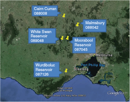
The study sites in central Victoria form a transect across a climatic, geographical and topographical gradient that influences the TWB. The stations were specifically selected along a north-south orientation stretching from the Victorian coastline, across the Great Divide and onto the northern inland plains (Fig. 1). The five stations have long-term rainfall and pan evaporation records which are largely complete with minimal missing data (Table 1).
|

|
2.2 Rainfall and pan evaporation data
All rainfall and pan evaporation data were obtained from the Bureau of Meteorology’s climate archive ADAM. Each station’s data records were analysed at a daily level with any (minimal) missing daily data infilled from the nearest neighbouring station in the case of rainfall.
When 5 days or fewer of pan evaporation were missing in a month, those days were infilled using the Silo data drill, a product from the QLD Department of Science, Information Technology, Innovation and the Arts (DSITIA). DSITIA developed a synthetic daily Class A pan evaporation data set for Australia for the period 1910–present, using a linear model and NR&M (Natural Resources and Mines) climate grids covering all of Australia at 0.05° (~5 km) spatial resolution. The resulting synthetic pan evaporation grids were calculated using a thin-plate spline algorithm to interpolate observed data supplied by the Bureau of Meteorology (Rayner 2005). Not all of the climate variables used to derive the synthetic pan evaporation data were directly observable (e.g. wind), so the resulting interpolated synthetic pan data was only used to infill up to five missing days per month. Thus monthly pan evaporation data containing minor gaps could be utilised to compile seasonal totals.
Rayner (2005) noted that the synthetic data struggled to capture extreme daily values of pan data, for example, high-evaporation days are underestimated and low-evaporation days are overestimated. A likely causal factor is the absence of wind input, with previous research finding average wind speed (wind run) to be the most significant influence on pan evaporation across much of Australia (Rayner 2007; Roderick et al. 2007; Johnson and Sharma 2010). This vindicates the cautious approach taken to infilling at the daily level, although the absence of wind input appears to have a negligible influence on synthetic pan evaporation values at longer timescales. Exploratory analysis in the study region showed the monthly-mean synthetic and observed pan evaporation values correlated at 0.96 without any systematic biases (Marshall 2016). In-filled synthetic data comprised <0.002% of the daily pan evaporation values used in this study.
2.3 Analysis period
The period of analysis for this research was primarily determined by the length and quality of data available. Specifically pan evaporation data posed several unique considerations, whereas the rainfall records at all stations were largely complete and extended well back into the early 20th century at most stations. In order to assess rainfall and pan evaporation characteristics over time, it was necessary to compare identical time periods. The earliest pan evaporation data occurred at Wurdiboluc Reservoir from 1969, whereas the last station to commence pan evaporation records was Cairn Curran in August 1972. Thus analysis starts from 1972, the first year in which pan evaporation records existed at all stations.
2.4 Climate indices
ENSO is a coupled atmospheric or oceanic phenomenon associated with zonal fluctuations in atmospheric pressure and circulation patterns across the Pacific Ocean. Numerous indices measuring oceanic characteristics are used to depict the strength of prevailing ENSO phases (Risbey et al. 2009).
Historically, ENSO events (La Niña and El Niño) have been associated with large-scale sea surface temperature (SST) anomalies in the western Pacific, a zone categorised as ‘Nino 4’, and the eastern Pacific (Nino 3). In particular, anomalies in the eastern sector have often been found to be useful indicators of basin-wide changes in ENSO phases. Since the 1970s ENSO events have exhibited some variation on this general principle, with the main area of SST anomalies tending to evolve further west in the central Pacific (5°N–5°S, 120–170°W) – a region known as ‘Nino 3.4’ (Brown et al. 2009; Risbey et al. 2009). For this study, the Nino 3.4 index is selected as the primary ENSO indicator, due to it having the strongest association with large-scale changes across the Pacific during our analysis period (Risbey et al. 2009). Monthly and seasonal Nino 3.4 data were obtained from the NOAA National Weather Service Climate Prediction Center.
The IOD is associated with atmospheric circulation changes resulting from west–east equatorial SST differences in the Indian Ocean (Saji et al. 1999). The Dipole Mode Index (DMI) measures the difference between SST anomalies in the western (50–70°E and 10°S–10°N) and eastern (90–110°E and 10–0°S) equatorial Indian Ocean and is widely used to monitor the IOD state. Monthly IOD data based on the DMI were obtained from the Bureau of Meteorology.
The SAM has been described using several parameters over various regions across differing data sets (Ho et al. 2012). Historically, the two most common methods of defining a SAM index have been to use either 700 or 850 hPa geopotential height anomalies, or mean sea level pressure (mslp) anomalies, between 65 or 70 and 40°S (Ho et al. 2012). Essentially, these indices describe the location of large-scale pressure and circulation anomalies that characterise each of the two SAM phases. That is, anomalously high pressure is seen over the mid-latitudes during +SAM with lower pressures at high latitudes, and the converse occurring during −SAM. This study utilises the Marshall Index of SAM obtained from https://legacy.bas.ac.uk/met/gjma/sam.html, accessed 7 February 2014.
3 Quality control
3.1 Siting and exposure
The significance of instrument exposure is particularly important for pan evaporation which is influenced by several atmospheric variables, including air temperature, solar radiation, relative humidity and wind flow. Although both pan evaporation and rainfall are influenced by broad-scale weather regimes, local modification of these conditions more readily affect pan evaporation through changes in the immediate environment. A prime example is the addition or removal of trees or other physical structures such as buildings, that markedly and suddenly change the exposure of the pan (van Dijk 1985; Jovanovic et al. 2008). Similarly, movement of the pan equipment to a different site can influence exposure, particularly if the new environment is not comparable to the original location, for example, a sheltered valley as opposed to an exposed ridge line. Jovanovic et al. (2008) found that some early studies of Australia’s pan evaporation trends had neglected to account for artificial changes to the pan’s exposure by using raw data without first referring to relevant metadata.
A check of historical metadata at each station was undertaken to discern whether significant changes to the pan instrument or the nearby environment could have adversely affected the pan evaporation data. Station reports of very detailed site diagrams back to the early 1990s were obtained from the Bureau of Meteorology and scrutinised (BOM 2013a–g). Significant changes to pan exposure were difficult to identify over this period unless explicitly documented.
An additional way to identify artificial changes in the immediate environment involves checking the raw data for abrupt changes in the mean value of the time series and which appear to be of a nonclimatic origin. Residual mass curves (RMCs) were used to detect change points in both rainfall and pan evaporation time series at stations in this study.
RMCs represent the cumulative sum of deviations from the long-term (1972–2013) mean and are constructed according to the following equation:
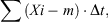
where Δt is the time step or time interval (in this case, monthly values); Xi is the ith element of the series, representing the average value over time interval Δt (mm/year), and m is the long-term average (1972–2013 mean), expressed in the same units as Xi (Rancic et al. 2009). When graphed, extremes of the RMCs associated with abrupt changes in the mean reflect sudden changes within the time series which are likely to be nonclimatic in origin, for example, change in location or exposure.
The RMCs detected anomalously low pan evaporation at Malmsbury and Wurdiboluc (relative to the 1972–2013 period) up until 1986 then markedly higher pan evaporation rates thereafter compared to the other stations. The two stations are separated by ~150 km and subject to vastly different climatic influences – Malmsbury is inland, elevated and with a northerly aspect, whereas Wurdiboluc is by the coast, surrounded by low undulating plains. Hence no common regional connection was identified which was peculiar to these stations. The increased pan evaporation at Wurdiboluc coincided with a marked increase in wind run, consistent with a relocation of the pan evaporation site in 1986 that resulted in greater wind exposure (Jovanovic et al. 2008). In compiling the HQ Australian Pan Evaporation data set, Jovanovic et al. (2008) applied an adjustment factor to the Wurdiboluc data prior to this pan relocation.
Using a similar but slightly different technique to Jovanovic et al. (2008), both the Wurdiboluc and Malmsbury records from 1972 to 1986 were adjusted using the change of mean from before and after the change point for each month. Mean seasonal adjustments for autumn, winter and spring were +9%, +9% and +7% at Wurdiboluc Reservoir; and +16%, +20% and +12% for Malmsbury (Marshall 2016). Following this adjustment, RMCs on the new homogenous data sets no longer showed any significant differences between the underexposed early records and the rest of the series. In all seasons, the time series of Wurdiboluc and Malmsbury now broadly exhibit deviations of pan evaporation regime similar to the other stations in the region (Fig. 2).

|
3.2 Bird guard corrections
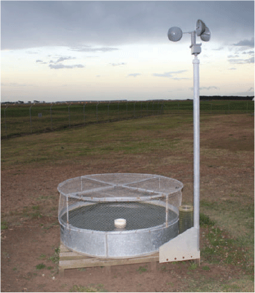
A change to the pan instrumentation, often overlooked in the literature (Jovanovic et al. 2008), was the installation of bird guards into the pan evaporation network across Australia which occurred predominantly during the early 1970s. A uniquely Australian modification, it sat on top of the pan itself and was fitted with chickenwire netting to restrict animal and bird access whilst still allowing pan water to interact with the air above. Field studies found that the installation of such structures acted to decrease exposure of the pan to elements like sunlight, wind and rainfall and modified the aerodynamic conditions immediately above the pan (Jovanovic et al. 2008). This had the effect of reducing pan evaporation by ~7% compared to unscreened pans (van Dijk 1985).
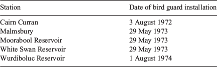
In the homogenisation process of Jovanovic et al. (2008), no adjustment of data before or after the installation of the bird guard was applied unless it was found to have had a significant and statistically identifiable effect on the data set, that is, it showed up as a change point in the mean of the series. Hence not all stations were subject to homogenisation processes resulting from the bird guard installation. For our network, the dates at which bird guards were installed at each station were obtained and a similar principle applied. All stations in our network had bird guards installed by July 1974, meaning pan evaporation data from 1975 onwards was obtained using comparable equipment (see Fig. 3 and Table 2). Again, the RMCs were utilised to see if there were significant and abrupt changes in the mean of the time series around that time. Taking the prevailing conditions into account, it was considered likely that at least some months prior to bird guard installation displayed very high pan evaporation values which could only be explained by the absence of the bird guard.
|
|
Hence the remaining three stations (Cairn Curran, Moorabool and White Swan) were corrected such that data before the bird guard installation was adjusted downwards by 7% as per the results of field trials by van Dijk (1985). No bird guard corrections were applied to Malmsbury or Wurdiboluc following their earlier homogenisation as neither site displayed excessively high values relative to the immediate years following the bird guard installation.
4 Methodology
4.1 Linear monthly trends
A linear fit was applied to each monthly time series to depict rainfall and pan evaporation trends at each station during 1972–2013. The trend line was derived using the least squares linear regression method as per Jovanovic et al. (2008).
The resulting trend line equation was used to quantify the monthly rainfall and pan evaporation trends at each station shown in Tables 4 and 5. Time series changes were expressed as both an absolute change (increase or decrease) in millimetres per decade and further as a percentage change per decade based on the respective month’s long-term mean. A two-tailed Student’s t-test was used to test statistical significance at the 95 per cent level (P < 0.05) of each longer term trend.
4.2 Correlation analysis
The association between rainfall or pan evaporation and prominent climate drivers (ENSO, IOD, SAM) is explored through correlation analysis at the monthly level using Pearson’s correlation coefficient R. Measuring the strength of the linear relationship between rainfall or pan evaporation and each respective climate driver, R values range from −1 to 1, with values closest to these two extremes indicative of a strong positive or negative relationship. Values close to zero reflect very weak relationships between variables. Statistically significant relationships are defined as those where R exceeded the 95th percentile and exhibited a P-value of <0.05. This generally meant that R values greater than 0.3 or −0.3 were of statistical significance with monthly correlations graphed to display the evolution of rainfall and pan evaporation relations with each climate driver throughout the growing season.
4.3 Composite analysis
ENSO and IOD events typically persist through much of the growing season once established. Seasonal composite analysis of rainfall and pan evaporation was performed for opposing phases of ENSO: La Niña and El Niño; and IOD: +IOD and −IOD. SAM was not analysed due to its variance between positive and negative phases on weekly and monthly timescales.
The thresholds for determining warm (El Niño, +IOD) and cold (La Niña, −IOD) phases for the composite analysis vary in the literature according to the specific ENSO or IOD indices used, for example, Meyers et al. (2007), Ummenhofer et al. (2009). Although there is general agreement in the literature as to what constitutes a La Niña or El Niño ‘year’, applying such broader definitions to a seasonal composite analysis could be misleading due to considerable variability in the timing and duration of La Niña or El Niño conditions throughout the growing season. ENSO or IOD conditions may only exist for short periods, with late starting ENSO events in spring, sometimes bearing little resemblance to the ENSO state that occurred in the preceding autumn and winter seasons.
Therefore, in order to fully reflect the varied influences of both drivers during the respective seasons, years where an ENSO or IOD event occurred have been determined based on particular thresholds being met as deviations from average conditions over that season. A typical threshold used by national meteorological agencies to categorise ENSO events, for example, is an SST index anomaly of ±0.5°C. In the composite analysis, this standard threshold is used to classify a seasonal ENSO event using Nino 3.4 indices, with the threshold increased to ±0.6°C from the long-term mean in spring to recognise the peak of ENSO conditions which are often experienced in this season (Table 3).
|
A similar seasonal threshold approach was applied to the IOD (DMI). It was found that by using thresholds similar to winter and spring when IOD has peak influence, there was a dearth of IOD years in autumn to allow for a reliable composite analysis in that season. Although this is predominantly a result of IOD events being largely undeveloped during autumn, it was considered important to still investigate the effects of IOD tendencies (despite the lack of discernible events) on rainfall and pan evaporation especially in light of the significant regional rainfall changes noted in recent decades during this season. Hence, the threshold for IOD phases was relaxed generally compared to ENSO, but particularly during autumn, to ensure an adequate number of years could be incorporated into the composite analysis. Although this method does not emphatically differentiate between ±IOD events, as it might with ENSO, it still allows for a comparison between opposing IOD tendencies even though the tendency itself may be classed as neutral in other seasons.
Seasonal box plots are constructed for La Niña or El Niño and −IOD or +IOD composites at each station and provide a visual representation of the range of rainfall and pan evaporation values that have occurred under the respective ENSO and IOD conditions during 1972–2013. The box plots are based on quartiles from the mean with outliers denoted by solid dots. A two-tailed Student’s t-test was used to test statistical significance at the 95 per cent level (P < 0.05).
5 Intraseasonal terrestrial water balance trends 1972–2013
5.1 Monthly rainfall trends
The autumn months display widespread rainfall declines at all stations (Table 4), with the exception of a slight increase at Cairn Curran in March. The percentage change is greatest in May with rainfall declining ~15% in the region through 1972–2013. As April and May are wetter months climatologically, such percentage reductions represent significantly larger rainfall deficits compared to March. This is consistent with previous research attributing the bulk of the autumn rainfall decline to these 2 months (Murphy and Timbal 2008; Kiem and Verdon-Kidd 2010; Cai et al. 2012; Cai and Cowan 2013). In May, the decline is statistically significant at all stations, but only so at Malmsbury in April.

|
The monthly rainfall trends in winter were statistically insignificant and generally weakly negative, although local variation existed between stations, for example, White Swan exhibited positive trends in June and July. Weak negative rainfall trends at all stations in August, which although statistically insignificant, were somewhat stronger than in June and July.
Spring rainfall trends displayed marked monthly variability. September rainfall exhibited weak-to-moderate negative trends across the region, with larger statistically significant declines observed at most stations in October. Interestingly, the rainfall decline in October was greater than that seen in May at some stations, with the decadal rate of decline as high as 19% at Malmsbury. Unlike April and May, analysis of any October rainfall decline is largely absent in the literature. November contrasted significantly with the earlier spring months, with increasing rainfall at all stations during 1972–2013. A distinct geographical gradient in the November trend magnitude is apparent, with the positive rainfall trend increasing further north. This suggests that the likely source of the increased November rainfall has its origins to the north of central Victoria.
5.2 Monthly pan evaporation trends
Monthly trends in pan evaporation (Table 5) displayed greater variation between stations and throughout the growing season. Stations along the Great Dividing Range exhibit decreasing pan evaporation trends throughout most months of the growing season. Although generally weak, the monthly pan evaporation declines occasionally reach statistical significance during autumn and early winter. In contrast, the coastal Wurdiboluc Reservoir has positive pan evaporation trends in all months except November. Weak and variable monthly trends exist inland at Cairn Curran, which displays a tendency towards increased pan evaporation throughout the spring which is generally not apparent elsewhere.

|
6 Large-scale climate driver associations with terrestrial water balance through the growing season
6.1 Rainfall correlations
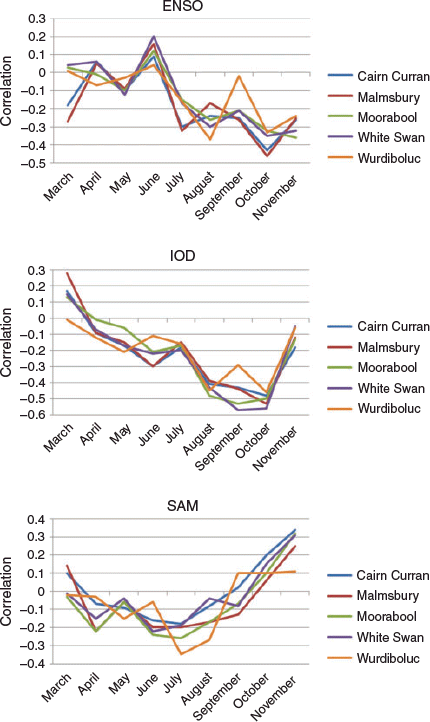
The influence of ENSO, IOD and SAM on growing season rainfall in central Victoria was analysed on an intraseasonal basis, using monthly correlations to provide an insight into the evolution of such relationships and short-term fluctuations occurring within the season.
The ENSO–rainfall relationship (Fig. 4) is mostly weak and variable in March when El Niño or La Niña events typically decay and conclude. Moderate negative correlations at the northern most stations (Cairn Curran and Malmsbury) likely reflect the final waning influence from any preceding ENSO event. Such ENSO effects disappear in April and May resulting in extremely weak rainfall correlations reflective of the overall autumn season. Positive ENSO correlations, although not statistically significant, exist at all stations in June before a moderate-to-strong negative rainfall relationship with ENSO tends to establish at all stations in July. This negative relationship exists through the remaining months of the growing season until November, with highest correlations occurring in October. A local anomaly occurs in September with Wurdiboluc displaying very weak correlations compared to the other stations. Despite the clear existence of a negative relationship between ENSO and rainfall after June, statistical significance is only reached throughout the region in October when monthly correlations are highest, as well as briefly at individual stations in July, August and November. Such low correlations indicate that although ENSO has an influence on rainfall from July to November, other large-scale drivers may exert a more prominent influence in the region.
|
In contrast to ENSO, evolution of the IOD’s influence on rainfall displays a much clearer, widespread and uniform signal within the growing season (Fig. 4). Weak negative correlations appear in April after being weakly positive in March. The negative correlations strengthen in early winter with statistical significance nearly reached at stations in the north (Cairn Curran and Malmsbury) during June. Saji et al. (1999) found the start of winter to be a common time for the expression of the first signs of an IOD event. The negative correlations temporarily weaken in July before increasing markedly in August and continuing to display strong to very strong and statistically significant rainfall correlations during September and October. The only exception is at Wurdiboluc where statistical significance briefly disappears in September, similar to ENSO during this month. After the very strong associations with rainfall during August–October, the IOD correlations fall abruptly below statistical significance in November, consistent with the notion that IOD events rarely continue into Summer due to the development of the southern hemisphere monsoon trough (Saji et al. 1999). Thus, significant tropical influence on growing season rainfall does not generally commence until mid-to-late winter (July for ENSO and August for IOD), with greatest impact on central Victorian rainfall seen in September and October before correlations decline in November.
The monthly cycle of SAM influence on rainfall is typified by weak correlations during the first half of the growing season similar to ENSO and IOD (Fig. 4). Weak negative correlations gradually strengthen during autumn and generally peak in mid-winter, reaching statistically significant levels at Wurdiboluc in July. The SAM correlations show a rapid weakening of the negative rainfall relationship in August before transitioning to positive correlations during September and October. These positive correlations strengthen into November reaching statistical significance at Cairn Curran, Moorabool and White Swan.
Although the magnitude of the correlations themselves are not remarkable, the unique change from negative-to-positive correlations at the start of spring are indicative of a rapid and significant switch in synoptic regime at this time. From March to August, −SAM (+SAM) is synonymous with higher (lower) rainfall, whereas the opposite is true during September–November. Both positive and negative SAM phases are capable of bringing substantial rainfall to SEA despite the processes behind such rainfall being very different (Hendon et al. 2007; Meneghini et al. 2007; Whan et al. 2013). This effect is particularly prominent during transition seasons like autumn and spring when pressure patterns undertake their seasonal migration north or south across SEA (Whan et al. 2013). In these seasons, when SAM is strongly negative, the mid-latitude storm belt moves northwards and brings rain bearing cold fronts and lows to SEA. However, when pressure patterns contract southwards enough during a significant +SAM phase, a strong easterly circulation prevails which often transports considerable amounts of moist air from the Pacific Ocean, increasing the chances of rainfall (Hendon et al. 2007; Meneghini et al. 2007; Whan et al. 2013).
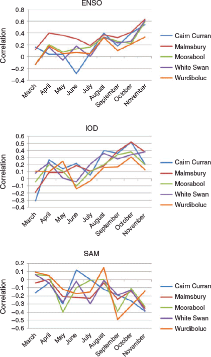
6.2 Pan evaporation correlations
Monthly analysis of pan evaporation correlations displayed much greater variance between stations than that observed with rainfall. This likely reflects the much greater sensitivity of pan evaporation to local effects under a given circulation regime, compared to rainfall.
The month-to-month relationship between ENSO and pan evaporation (Fig. 5) is generally weak and variable from March to July, although local anomalies are evident at Malmsbury where statistically significant positive correlations occur in April and May. An increased ENSO influence on pan evaporation occurs in winter, becoming prominent in August, a month later than the corresponding ENSO effect on rainfall. Correlations generally ease in September before increasing in October and reaching statistical significance throughout the region in November, with very strong ENSO–pan evaporation correlations across the Great Dividing Range.
|
The monthly IOD correlations (Fig. 5) exhibit broad similarities to ENSO with no strong association with pan evaporation apparent until August, coinciding with an increased IOD influence on rainfall. Positive IOD–pan evaporation correlations increase in spring and, like rainfall, generally peak in October. IOD influence along the coast at Wurdiboluc is subdued somewhat with statistical significance never reached in any of the spring months. Although the ENSO correlations with pan evaporation develop further in November, the IOD influence diminishes, though not as dramatically as that seen with rainfall.
The SAM–pan evaporation relationship displays large and variable fluctuations from month to month throughout the region (Fig. 5). Despite the high monthly variance, the SAM association with pan evaporation remains mostly negative and generally increases over the growing season. In spite of the rather erratic monthly correlations, the peak SAM effect on pan evaporation is considerably greater than that on rainfall, with the occurrence of statistically significant pan evaporation correlations in September and November as high as r = −0.49 at Wurdiboluc Reservoir. Despite temporarily strong correlations, there appears no systematic growing season evolution of the SAM relationship with pan evaporation at a regional scale, like that observed with the IOD and ENSO. There is also no reversal of SAM–pan evaporation relationship, for example, negative to positive, like that seen with rainfall at the beginning of spring.
7 The effects of El Niño–Southern Oscillation and Indian Ocean Dipole years on rainfall and pan evaporation
7.1 Rainfall composites
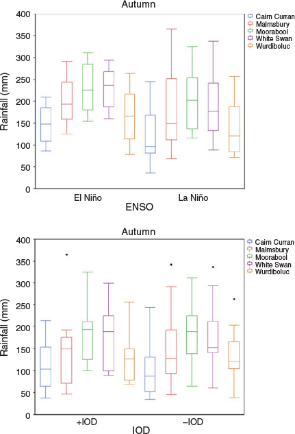
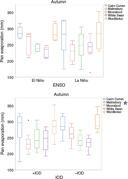
As discussed in Section 4, the composite analysis of ENSO and IOD years in autumn must be viewed in a different light to those in winter and spring, due to a rarity of La Niña or El Niño, or −IOD or +IOD events in this season. Thus, autumn is the time of year when ENSO and IOD have least impact on SEA climate, illustrated earlier by the low monthly correlations with rainfall and pan evaporation at all stations. Hence, the autumn analysis depicts conditions where ENSO and IOD ‘tendencies’ are apparent, but at a much lower threshold than during winter and spring.
Figure 6 displays no major differences in mean rainfall between opposing ENSO and IOD phases in autumn. The lack of a clear ENSO or IOD signal in this season is reflected in the indifferent rainfall variations observed under each respective ENSO and IOD phase. In autumn, it appears that conditions usually associated with reduced rainfall later in the growing season (El Niño, +IOD) tend to display slightly higher rainfall on the average, compared to traditionally wetter phases (La Niña and −IOD). Overall the probability of receiving high rainfall in autumn is neither enhanced or reduced by ENSO or IOD, consistent with previous research that suggests that the long-term rainfall decline in this season is unlikely to be attributed to changes in these particular drivers (Murphy and Timbal 2008).
|
Although no significant difference in mean rainfall exists between ENSO states in autumn, an asymmetry exists in terms of rainfall variability under each phase. Specifically, the autumn rainfall spread under La Niña conditions is much greater than during El Niño. The greater La Niña variability results from both high and low rainfall autumns occurring under strong La Niña conditions, whereas the El Niño rainfall response is generally much more linear. Asymmetrical Australian rainfall responses to ENSO have previously been noted by Power et al. (2006) during June–December, but not in autumn. Nonlinearity in rainfall variability associated with ENSO was also evident in the winter composites (Fig. 7), consistent with Power et al. (2006). This asymmetrical rainfall response is the opposite of that seen in autumn with markedly reduced variability observed during La Niña phases.
|
Consistent with Risbey et al. (2009), the winter composite analysis did not elicit a significant mean rainfall difference between ENSO phases, despite the much greater rainfall variance during El Niño compared to La Niña. Similarly, Brown et al. (2009) found that the presence of El Niño need not necessarily equate to low growing season rainfall in SEA. Their examination of three El Niño years (1982, 1997 and 2002) found that the strength of El Niño conditions were not always reflected in subsequent rainfall anomalies; however, such effects could vary significantly between seasons. For instance, the very strong 1997 El Niño saw a very dry winter followed by near-average rainfall in spring, whereas the relatively weak El Niño in 2002 displayed marked rainfall deficiencies throughout both seasons (Brown et al. 2009).
In the correlation analysis, the IOD exerted a greater influence on central Victorian winter rainfall than ENSO. Although previous research suggested that the IOD may act as a pathway through which ENSO impacts SEA rainfall (Cai et al. 2011), Risbey et al. (2009) demonstrated that June–October IOD correlations with SEA rainfall remained high after the relationship with ENSO was removed using partial correlations. Conversely, ENSO correlations with SEA rainfall dissipated once the IOD influence was removed. Such findings suggest that the IOD association with rainfall is able to operate independently of ENSO, but that ENSO’s effect on SEA rainfall can be expressed via the IOD due to the frequent co-occurrence of warm or cold phases of each driver. Hence, the greater IOD influence in winter is reflected in statistically significant (P < 0.05) rainfall differences between positive and negative phases at all stations. Higher rainfall in SEA during −IOD years is associated from increased moisture flux across the country from the northwest compared to +IOD years (Ummenhofer et al. 2009).
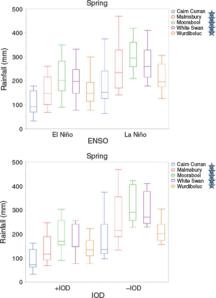
Statistically significant spring rainfall correlations with ENSO and IOD were evident at all stations during 1972–2013, coincident with the period of the annual cycle when ENSO and IOD events often reach maximum intensity and hence exert the greatest direct influence on SEA climate. The spring rainfall composite analysis (Fig. 8) reflects this with statistically significant differences at all stations between opposing ENSO and IOD events. La Niña and −IOD spring seasons exhibit much higher mean rainfall than El Niño and +IOD, consistent with previous SEA studies into ENSO or IOD effects on spring rainfall (Meyers et al. 2007; Murphy and Timbal 2008; Risbey et al. 2009; Ummenhofer et al. 2009, 2010).
|
Although the simultaneous occurrence of wet or dry phases in both the Pacific and Indian Oceans reliably translates into higher or lower spring rainfall anomalies, it has been noted that La Niña or −IOD and El Niño or +IOD in combination do not necessarily enhance spring rainfall anomalies beyond what is experienced if only one of the drivers are in a wet phase (Meyers et al. 2007; Risbey et al. 2009; Ummenhofer et al. 2010).
7.2 Pan evaporation composites
Composite analysis of La Niña or El Niño and −IOD or +IOD tendencies showed no statistically significant pan evaporation differences (Fig. 9) during autumn, consistent with the rainfall composites which also found minimal effect from ENSO and IOD in this season. An exception was at Malmsbury which displayed statistically significant pan evaporation differences between IOD regimes, with higher pan evaporation occurring when the IOD was negative. Similar to the autumn rainfall composites, pan evaporation exhibited much greater variability under La Niña conditions compared to El Niño.
|
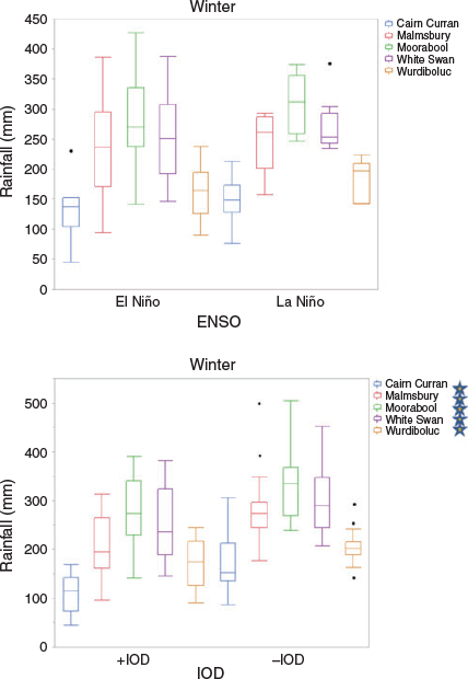
Winter pan evaporation characteristics during ENSO and IOD events broadly reflect the increased influence seen with each driver in the correlation analysis. Thus, statistically significant pan evaporation differences between ENSO phases are evident at all stations except Cairn Curran in winter (Fig. 10). Higher pan evaporation during El Niño compared to La Niña, being a reflection of the change in moisture fluxes, cloud cover and rainfall associated with each regime.
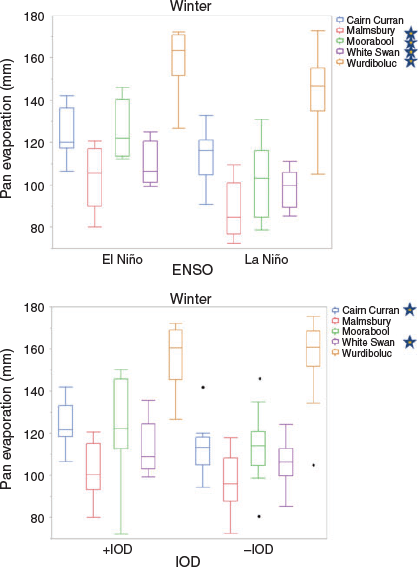
|
The clear pan evaporation differences between La Niña and El Niño in winter, contrasts with the rainfall composite analysis, which exhibited much stronger relations to the prevailing IOD phase, rather than ENSO in this season. Conversely, minimal differences in winter pan evaporation is evident in the IOD composites, although two stations (Cairn Curran and White Swan) displayed statistically significant differences between IOD phases. The variable and generally opposing impacts of ENSO or IOD composites on winter rainfall and pan evaporation suggest that the often complimentary relationship between rainfall and pan evaporation fails to operate in any consistent capacity during this season. For example, higher rainfall under −IOD conditions do not necessarily appear to be accompanied by a reduced rate of pan evaporation. Such findings indicate variability in the overall TWB response during winter, despite rainfall and pan evaporation components showing strong in-phase associations with ENSO and IOD.
Seasonally, the spring composites display the most marked and statistically significant pan evaporation differences across central Victoria for both ENSO and IOD (Fig. 11), consistent with strong correlations with both drivers in this season. The large-scale changes in circulation associated with each driver means that conditions that bring increased cloud cover and relative humidity (La Niña, −IOD) promote greater rainfall and reduced pan evaporation, whereas phases responsible for drier air, increased solar exposure and higher temperatures (El Niño, +IOD) generate lower rainfall and greater pan evaporation (Roderick and Farquhar 2004; Jovanovic et al. 2008; Roderick et al. 2009b). Thus, the complimentary association between rainfall and pan evaporation is greatest in spring at all stations and in nearly all instances is statistically significant.
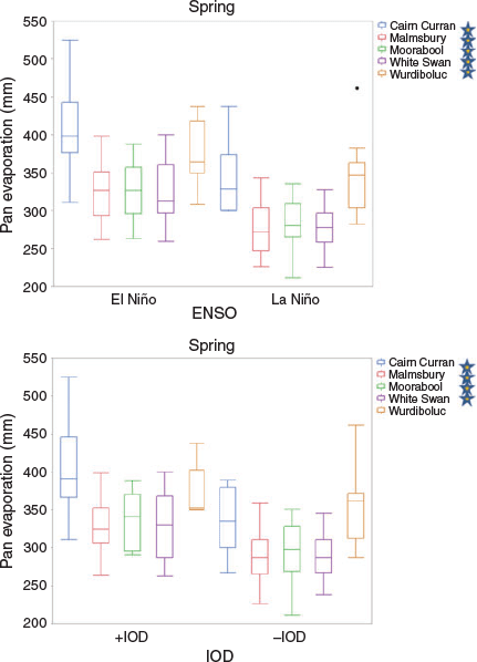
|
Conclusions
Growing season (March–November) rainfall and pan evaporation characteristics have been examined at stations within a north-south climatic gradient in central Victoria. The five stations were analysed at both monthly and seasonal scales between 1972 and 2013.
Autumn has seen a long-term reduction in rainfall at all stations across 1972–2013, which is statistically significant and greatest in April and May. Consistent with previous research, no strong connection was found with ENSO, IOD or SAM to explain the cause of this decline (Meneghini et al. 2007; Murphy and Timbal 2008; Risbey et al. 2009; Cai and Cowan 2013). Most stations also exhibited decreasing pan evaporation during this season, though of a smaller magnitude than rainfall. Over the analysis period, autumn pan evaporation shows statistically significant correlations with the SAM, except on the Victorian coastline. Hence the increasingly +SAM trend in autumn may be contributing to the long-term decline in pan evaporation through increasingly calm and stable conditions, despite only a weak association with rainfall.
Trends in winter rainfall and pan evaporation were relatively minor with both exhibiting a weak decline at most stations, with the rainfall reduction most evident in August. The climate driver with the greatest influence on rainfall is the IOD, particularly at inland stations owing to their greater exposure to northwest airstreams originating from the Indian Ocean (Meyers et al. 2007; Risbey et al. 2009; Cai et al. 2011). Statistically significant differences in winter rainfall between negative and positive IOD conditions were apparent at all stations. Winter pan evaporation displayed the highest correlations with ENSO, exhibiting significantly less pan evaporation under La Niña conditions compared to El Niño. The contrast in pan evaporation between the two ENSO states is likely to reflect changes associated with tropical moisture flux into the region and hence cloud cover and humidity. The influence of ENSO and IOD on rainfall and pan evaporation was more prominent in August, with only weak TWB relations during June and July.
The strongest correlations with all climate drivers were evident in spring, as well as the greatest interannual variability in rainfall and pan evaporation. Rainfall was very strongly correlated to the IOD, whilst also being statistically significant with ENSO. This is consistent with previous research which found IOD and ENSO states often covary, particularly in spring (Meyers et al. 2007; Risbey et al. 2009). Thus, La Niña and −IOD commonly occur simultaneously, likewise El Niño and +IOD. The frequent pairing of similar Pacific and Indian Ocean states has previously caused debate over the interdependence of IOD from ENSO, as well as the role of the Indian Ocean in transmitting ENSO influence to SEA (Saji et al. 1999; Meyers et al. 2007; Risbey et al. 2009; Ummenhofer et al. 2009). During 1972–2013, the months of September and especially October experienced significant rainfall declines, whereas November rainfall increased. Despite the monthly variation, negative trends in total spring rainfall were observed, although the magnitude of the decline is somewhat exaggerated by the presence of very high rainfall years at the beginning of the analysis. However, contributing to a general spring rainfall decline has also been a marked reduction in the frequency of wet conditions and the occurrence of several very low rainfall years after 2001. These very low rainfall years have coincided with an increased frequency of +IOD events (Ummenhofer et al. 2010), resulting in suppressed tropical moisture flux accompanying synoptic systems affecting SEA. Although the mechanisms by which IOD conditions produce rainfall fluctuations in SEA are well understood (Meyers et al. 2007; ), it was found that the IOD and ENSO influence also has a statistically significant association with spring pan evaporation. Composite analysis showed markedly lower pan evaporation under La Niña and −IOD, likely due to greater cloud cover, humidity and rainfall, compared to the drier, warmer and generally greater solar radiation levels received during El Niño and +IOD (Ummenhofer et al. 2010). The strongly inverse rainfall–pan evaporation relationship in spring means that the magnitude of wet and dry TWB conditions are magnified according to the prevailing ENSO or IOD phase. This may have particular significance for analysing drought conditions, where common assessment of rainfall deviations from the mean can sometimes fail to fully illustrate the overall moisture deficits which are accruing during El Niño and +IOD phases. Overall trends in spring pan evaporation were generally weak and variable from month to month and between stations.
This research has emphasised the need to understand the pan evaporation element of the TWB in concert with rainfall, building on the rather limited literature concerning pan evaporation characteristics and trends in Australia. Previous studies have often focused on pan evaporation at the continental level and on an annual basis, whereas this research has examined local variations within a regional area at the monthly and seasonal scale, as well as the response of pan evaporation characteristics to changes in large-scale climate drivers. Previous research has focussed on the pan evaporation affects from directly measured elements such as air temperature and rainfall (Rayner 2007; Roderick et al. 2007; Johnson and Sharma 2010), often reflecting conditions within the immediate station vicinity. In this study, pan evaporation generally observed stronger correlations with climate drivers than that seen with rainfall. Hence, the future utilisation of such strong relationships may be possible for the seasonal forecasting of pan evaporation similar to rainfall, providing a more complete picture of TWB conditions for agricultural and related industries in central Victoria.
Acknowledgements
The author thanks Professor Peter Gell (Federation University) for his advice and suggestions in preparing this paper. This research did not receive any specific funding.
References
Ashcroft, L., Karoly, D., and Gergis, J. (2012). Temperature variations of southeastern Australia, 1860–2011. Aust. Meteorol. Oceanogr. J. 62, 227–245.| Temperature variations of southeastern Australia, 1860–2011.Crossref | GoogleScholarGoogle Scholar |
Brown, J. N., McIntosh, P. C., Pook, M. J., and Risbey, J. S. (2009). An investigation of the links between ENSO flavours and rainfall processes in southeastern Australia. Mon. Wea. Rev. 137, 3786–3795.
| An investigation of the links between ENSO flavours and rainfall processes in southeastern Australia.Crossref | GoogleScholarGoogle Scholar |
Bureau of Meteorology (BOM) (2006). Special Climate Statement 9 – An exceptionally dry decade in parts of southern and eastern Australia: October 1996 – September 2006. Issued 10th October 2006. pp. 9. (National Climate Centre.) Available at http://www.bom.gov.au/climate/current/statements/scs9a.pdf [Verified 22 April 2020].
Bureau of Meteorology (BOM) and CSIRO (2012). State of the Climate 2012. 12 pp. Available at http://www.bom.gov.au/announcements/media_releases/ho/stateClimate2012.pdf [Verified 22 April 2020].
Bureau of Meteorology (BOM) (2013a). Basic Climatological Station Metadata: Cairn Curran 088009. Available at http://www.bom.gov.au/clim_data/cdio/metadata/pdf/siteinfo/IDCJMD0040.088009.SiteInfo.pdf [Verified 22 April 2020].
Bureau of Meteorology (BOM) (2013b). Basic Climatological Station Metadata: Malmsbury 088042. Available at http://www.bom.gov.au/clim_data/cdio/metadata/pdf/siteinfo/IDCJMD0040.088042.SiteInfo.pdf [Verified 22 April 2020].
Bureau of Meteorology (BOM) (2013c). Basic Climatological Station Metadata: Moorabool Reservoir 087045. Available at http://www.bom.gov.au/clim_data/cdio/metadata/pdf/siteinfo/IDCJMD0040.087045.SiteInfo.pdf [Verified 22 April 2020].
Bureau of Meteorology (BOM) (2013d). Basic Climatological Station Metadata: White Swan Reservoir 089048. Available at http://www.bom.gov.au/clim_data/cdio/metadata/pdf/siteinfo/IDCJMD0040.089048.SiteInfo.pdf [Verified 22 April 2020].
Bureau of Meteorology (BOM) (2013e). Basic Climatological Station Metadata: Durdidwarrah 087021. Available at http://www.bom.gov.au/clim_data/cdio/metadata/pdf/siteinfo/IDCJMD0040.087021.SiteInfo.pdf [Verified 22 April 2020].
Bureau of Meteorology (BOM) (2013f). Basic Climatological Station Metadata: Geelong Salines 087023. Available at http://www.bom.gov.au/clim_data/cdio/metadata/pdf/siteinfo/IDCJMD0040.087023.SiteInfo.pdf [Verified 22 April 2020].
Bureau of Meteorology (BOM) (2013g). Basic Climatological Station Metadata: Wurdiboluc Reservoir 087126. Available at http://www.bom.gov.au/clim_data/cdio/metadata/pdf/siteinfo/IDCJMD0040.087126.SiteInfo.pdf [Verified 22 April 2020].
Cai, W., Rensch, P. V., and Cowan, T. (2011). Influence of global-scale variability on the subtropical ridge over Southeast Australia. J. Clim. 24, 6035–6053.
| Influence of global-scale variability on the subtropical ridge over Southeast Australia.Crossref | GoogleScholarGoogle Scholar |
Cai, W., Cowan, T., and Thatcher, M. (2012). Rainfall reductions over southern hemisphere semi-arid regions: the role of subtropical dry zone expansion. Sci. Rep. 2, 1–5.
| Rainfall reductions over southern hemisphere semi-arid regions: the role of subtropical dry zone expansion.Crossref | GoogleScholarGoogle Scholar |
Cai, W., and Cowan, T. (2013). Southeast Australia autumn rainfall reduction: a climate-change-induced poleward shift of ocean–atmosphere circulation. J. Clim. 26, 189–205.
| Southeast Australia autumn rainfall reduction: a climate-change-induced poleward shift of ocean–atmosphere circulation.Crossref | GoogleScholarGoogle Scholar |
Fu, G., Charles, S. P., and Yu, J. (2009). A critical overview of pan evaporation trends over the last 50 years. Clim. Change 97, 193–214.
| A critical overview of pan evaporation trends over the last 50 years.Crossref | GoogleScholarGoogle Scholar |
Hendon, H. H., Thompson, D. W. J., and Wheeler, M. C. (2007). Australian rainfall and surface temperature variations associated with the southern hemisphere annular mode. J. Clim. 20, 2452–2467.
| Australian rainfall and surface temperature variations associated with the southern hemisphere annular mode.Crossref | GoogleScholarGoogle Scholar |
Ho, M., Kiem, A. S., and Verdon-Kidd, D. C. (2012). The southern annular mode: a comparison of indices. Hydrol. Earth Syst. Sci. 16, 967–982.
| The southern annular mode: a comparison of indices.Crossref | GoogleScholarGoogle Scholar |
Hobbins, M. T., Dai, A., Roderick, M. L., and Farquhar, G. D. (2008). Revisiting the parameterization of potential evaporation as a driver of long-term water balance trends. Geophys. Res. Lett. 35, 1–6.
| Revisiting the parameterization of potential evaporation as a driver of long-term water balance trends.Crossref | GoogleScholarGoogle Scholar |
Johnson, F., and Sharma, A. (2010). A comparison of Australian open water body evaporation trends for current and future climates estimated from Class A evaporation pans and general circulation models. J. Hydrometeorol. 11, 105–121.
| A comparison of Australian open water body evaporation trends for current and future climates estimated from Class A evaporation pans and general circulation models.Crossref | GoogleScholarGoogle Scholar |
Jovanovic, B., Jones, D. A., and Collins, D. (2008). A high quality monthly pan evaporation dataset for Australia. Clim. Change 87, 517–535.
| A high quality monthly pan evaporation dataset for Australia.Crossref | GoogleScholarGoogle Scholar |
Kiem, A. S., and Verdon-Kidd, D. C. (2010). Towards understanding hydroclimatic change in Victoria, Australia – preliminary insights into the “Big Dry”. Hydrol. Earth Syst. Sci. 14, 433–445.
| Towards understanding hydroclimatic change in Victoria, Australia – preliminary insights into the “Big Dry”.Crossref | GoogleScholarGoogle Scholar |
Marshall, A. J. (2016). Precipitation and evaporative aspects of the terrestrial water balance in Central Victoria and their relationship to large-scale climate drivers during the growing season. Masters Thesis, University of Ballarat/Federation University, Australia. Available at https://researchonline.federation.edu.au/vital/access/manager/Repository/vital:10828 [Verified 22 April 2020].
Meneghini, B., Simmonds, I., and Smith, I. N. (2007). Association between Australian rainfall and the Southern Annular Mode. Int. J. Climatol. 27, 109–121.
| Association between Australian rainfall and the Southern Annular Mode.Crossref | GoogleScholarGoogle Scholar |
Meyers, G., McIntosh, P., Pigot, L., and Pook, M. (2007). The years of El Niño, La Niña and interaction with the Indian Ocean. J. Clim. 20, 2872–2880.
| The years of El Niño, La Niña and interaction with the Indian Ocean.Crossref | GoogleScholarGoogle Scholar |
Murphy, B. F., and Timbal, B. (2008). A review of recent climate variability and climate change in southeastern Australia. Int. J. Climatol. 28, 859–879.
| A review of recent climate variability and climate change in southeastern Australia.Crossref | GoogleScholarGoogle Scholar |
Nicholls, N. (2004). The changing nature of Australian droughts. Clim. Change 63, 323–336.
| The changing nature of Australian droughts.Crossref | GoogleScholarGoogle Scholar |
Power, S., Haylock, M., Colman, R., and Wang, X. (2006). The predictability of interdecadal changes in ENSO activity and ENSO teleconnections. J. Clim. 19, 4755–4771.
| The predictability of interdecadal changes in ENSO activity and ENSO teleconnections.Crossref | GoogleScholarGoogle Scholar |
Rancic, A., Salas, G., Kathuria, A., Acworth, I., Johnston, W., Smithson, A., and Beale, G. (2009). Climatic influence on shallow fractured-rock groundwater systems in the Murray–Darling Basin, NSW. (NSW Department of Environment and Climate Change.) Available at http://www.environment.nsw.gov.au/resources/salinity/09108groundwatermdb.pdf [Verified 22 April 2020].
Rayner, D. P. (2005). Australian synthetic daily Class A pan evaporation – technical report December 2005. (Queensland Department of Natural Resources and Mines.) Available at https://www.longpaddock.qld.gov.au/silo/documentation/AustralianSyntheticDailyClassAPanEvaporation.pdf [Verified 22 April 2020].
Rayner, D. P. (2007). Wind run changes: the dominant factor affecting pan evaporation trends in Australia. J. Clim. 20, 3379–3394.
| Wind run changes: the dominant factor affecting pan evaporation trends in Australia.Crossref | GoogleScholarGoogle Scholar |
Risbey, J. S., Pook, M. J., McIntosh, P. C., Wheeler, M. C., and Hendon, H. H. (2009). On the remote drivers of rainfall variability in Australia. Mon. Wea. Rev. 137, 3233–3253.
| On the remote drivers of rainfall variability in Australia.Crossref | GoogleScholarGoogle Scholar |
Roderick, M. L., and Farquhar, G. D. (2002). The cause of decreased pan evaporation over the past 50 years. Sci. Mag. 298, 1410–1411.
| The cause of decreased pan evaporation over the past 50 years.Crossref | GoogleScholarGoogle Scholar |
Roderick, M. L., and Farquhar, G. D. (2004). Changes in Australian pan evaporation from 1970 to 2002. Int. J. Climatol. 24, 1077–1090.
| Changes in Australian pan evaporation from 1970 to 2002.Crossref | GoogleScholarGoogle Scholar |
Roderick, M. L., Rotstayn, L. D., Farquhar, G. D., and Hobbins, M. T. (2007). On the attribution of changing pan evaporation. Geophys. Res. Lett. 34, 1–6.
| On the attribution of changing pan evaporation.Crossref | GoogleScholarGoogle Scholar |
Roderick, M. L., Hobbins, M. T., and Farquhar, G. D. (2009a). Pan evaporation trends and the terrestrial water balance. I. Principles and observations. Geogr. Compass 3/2, 746–760.
| Pan evaporation trends and the terrestrial water balance. I. Principles and observations.Crossref | GoogleScholarGoogle Scholar |
Roderick, M. L., Hobbins, M. T., and Farquhar, G. D. (2009b). Pan evaporation trends and the terrestrial water balance. II. Energy balance and interpretation. Geogr. Compass 3/2, 761–780.
| Pan evaporation trends and the terrestrial water balance. II. Energy balance and interpretation.Crossref | GoogleScholarGoogle Scholar |
Saji, N. H., Goswami, B. N., Vinayachandran, P. N., and Yamagata, T. (1999). A dipole mode in the tropical Indian Ocean. Nature 401, 360–363.
| A dipole mode in the tropical Indian Ocean.Crossref | GoogleScholarGoogle Scholar |
Timbal, B., Arblaster, J., Braganza, K., Fernandez, E., Hendon, H., Murphy, B., Raupach, M., Rakich, C., Smith, I., Whan, K., and Wheeler, M. (2010). Understanding the anthropogenic nature of the observed rainfall decline across South Eastern Australia. CAWCR technical report no. 026. Available at http://www.cawcr.gov.au/publications/technicalreports/CTR_026.pdf [Verified 22 April 2020].
Timbal, B., and Fawcett, R. (2012). A historical perspective on southeastern Australian Rainfall since 1865 using the instrumental record. J. Clim. 26, 1112–1129.
| A historical perspective on southeastern Australian Rainfall since 1865 using the instrumental record.Crossref | GoogleScholarGoogle Scholar |
Trewin, B., and Vermont, H. (2010). Changes in the frequency of record temperatures in Australia, 1957–2009. Aust. Meteorol. Oceanogr. J. 60, 113–119.
| Changes in the frequency of record temperatures in Australia, 1957–2009.Crossref | GoogleScholarGoogle Scholar |
Ummenhofer, C. C., England, M. H., McIntosh, P. C., Meyers, G. A., Pook, M. J., Risbey, J. S., Sen Gupta, A., and Taschetto, A. S. (2009). What causes southeast Australia’s worst droughts? Geophys. Res. Lett. 36, 1–5.
| What causes southeast Australia’s worst droughts?Crossref | GoogleScholarGoogle Scholar |
Ummenhofer, C. C., Sen Gupta, A., Briggs, P. R., England, M. H., McIntosh, P. C., Meyers, G. A., Pook, M. J., Raupach, M. R., and Risbey, J. S. (2010). Indian and Pacific Ocean influences on southeast Australian drought and soil moisture. J. Clim. 24, 1313–1336.
| Indian and Pacific Ocean influences on southeast Australian drought and soil moisture.Crossref | GoogleScholarGoogle Scholar |
van Dijk, M. H. (1985). Reduction in evaporation due to the bird screen used in the Australian class A pan evaporation network. Austr. Meteorol. Mag. 33, 181–183.
Verdon-Kidd, D. C., and Kiem, A. S. (2009a). Nature and causes of protracted droughts in southeast Australia: comparison between the Federation, WWII, and Big Dry droughts. Geophys. Res. Lett. 36, L22707.
| Nature and causes of protracted droughts in southeast Australia: comparison between the Federation, WWII, and Big Dry droughts.Crossref | GoogleScholarGoogle Scholar |
Verdon-Kidd, D. C., and Kiem, A. S. (2009b). On the relationship between large-scale climate modes and regional synoptic patterns that drive Victorian rainfall. Hydrol. Earth. Syst. Sci. 13, 467–479.
| On the relationship between large-scale climate modes and regional synoptic patterns that drive Victorian rainfall.Crossref | GoogleScholarGoogle Scholar |
Verdon-Kidd, D. C., Kiem, A. S., and Moran, R. (2014). Links between the Big Dry in Australia and hemispheric multi-decadal climate variability. Hydrol. Earth. Syst. Sci. 18, 2235–2256.
| Links between the Big Dry in Australia and hemispheric multi-decadal climate variability.Crossref | GoogleScholarGoogle Scholar |
Whan, K., Bertrand Timbal, B., and Lindesay, J. (2013). Linear and nonlinear statistical analysis of the impact of sub-tropical ridge intensity and position on south-east Australian rainfall. Int. J. Climatol. 34, 326–342.
| Linear and nonlinear statistical analysis of the impact of sub-tropical ridge intensity and position on south-east Australian rainfall.Crossref | GoogleScholarGoogle Scholar |