Simulating wildfire spread based on continuous time series remote sensing images and cellular automata
Huajian Zhuang A B , Naian Liu A B * , Xiaodong Xie A B * , Xuan Xu A B , Mengmeng Li A B , Yang Zhang A B and Rui Wang CA
B
C
Abstract
Acquiring behaviour parameters of wildfire propagation and developing firefighting strategies necessitate a precise and efficient simulation method; fireline coordinates and rate of spread (ROS) are two crucial parameters closely associated with simulation precision.
This study proposes an adaptive simulation method for wildfire propagation by integrating continuous time series remote sensing images with a cellular automata (CA) model.
The ROS in each direction is calculated using continuous time fireline coordinates derived from multi-source remote sensing images. A time-adaptive propagation algorithm is developed based on the CA model (time-adaptive cellular automata, TCA). Vegetation distribution information is derived to establish a simulation system for verification experiments.
The TCA model demonstrated satisfactory simulation performance, with a prediction accuracy of 92.2% for burned area and 87.3% for fireline length within local regions in the MuLi Forest Fire and effectively characterised gradual spread based on low ROS.
The adaptive simulation method produces fairly precise results and demonstrated its capability to achieve localised and gradual propagation. This software serves as a powerful tool for wildland surface fire prevention and control.
The adaptive simulation method based on continuous time remote sensing images and the CA model are essential for accurately predicting wildfire propagation.
Keywords: cellular automata model, continuous-time remote sensing images, coordinates of fireline, rate of spread, simulation of wildfire propagation, simulation software, vegetation inversion, wildfire spread rules.
Introduction
In recent years, wildfires have emerged as a growing global concern, causing significant damage to the structure, composition and functionality of pristine forests while also posing threats to human security and regional economies (McNamee et al. 2019; Crist 2023; Mitchell 2023; Woinarski et al. 2023). The accurate simulation of wildfire propagation is crucial for obtaining real-time fire spread information and devising effective firefighting strategies (Meng et al. 2023). Wildfire propagation simulation has been performed using various models. An empirical model typically establishes mathematical relationships between the geographic parameters and the rate of fire spread (ROS) through experimental analysis. For instance, Noble et al. (1980) developed a comprehensive fire statistics table by conducting over 800 experiments in Australian forests and grasslands with flat topography. The wildfire spread model proposed by Junpen et al. (2013) utilises a statistical approach based on multiple fire experiments, specifically designed for the foliage in northern Thailand. However, it should be noted that the effectiveness of the models mentioned above depends highly on the diverse geographical characteristics of each country. In contrast, Rothermel (1972) developed a method for calculating fire spread rates based on the principle of energy conservation, which involves heating unburned fuel ahead of the flame front until its temperature reaches the ignition point. The cellular automata (CA) model (Clarke et al. 1994) is another well-known semi-empirical model that is appreciated for its simple structure and computational efficiency for wildfire spread modelling. For example, Sun et al. (2021) incorporated a time factor into the Wang model (Wang 1992) to simulate wildfire spread using a CA model, whereas Gharakhanlou and Hooshangi (2021) introduced dynamic wind speed and direction into the simulation and utilised a genetic algorithm (GA) correction (Sohail 2023) based on a CA model. Most CA models calculate the ROS by incorporating geographical parameters within a grid to implement propagation techniques, yet they lack the integration of actual wildfire behaviour parameters into the propagation to guide models. This limitation hinders the accurate characterisation of uncontrollable variables in wildfires.
With advances in remote sensing technology, researchers have integrated remote sensing images of wildfires with fire propagation models to enhance their performance. Zheng et al. (2017) integrated the CA model with the extreme learning machine (ELM) to infer the local conversion rules for forest fire spread using historical data. Cruz et al. (2021) developed a fire spread model with different fire intensities based on experimental and actual wildfire data. Incorporating wildfire remote sensing images into fire spread models has proved successful, greatly enhancing their effectiveness. However, the relevant methods primarily focus on static spatial information post wildfire. Some optimised models encounter specific limitations, particularly in accurately predicting ongoing local wildfire spread.
Considering the above limitations, the present study proposes an adaptive simulation method to enhance the precision of wildfire propagation simulation by integrating continuous time series remote sensing images and a CA model. Specifically, a case study utilises continuous time series remote sensing images of the MuLi Forest Fire in Liangshan Prefecture, Sichuan Province on 28 March 2020 to extract the coordinates of the fireline and determine the average ROS in each direction. The coordinates of the fireline and the average ROS are then used as initial inputs for simulation purposes. A time-adaptive CA model is proposed to accurately simulate wildfire spread with a lower ROS within localised regions. Further, we employ an inverted spatial distribution analysis of vegetation within the research area. Subsequently, we develop a simulation system for predicting wildfire propagation that integrates the continuous time series remote sensing images, the time-adaptive cellular automata (TCA) model and the inversion results for vegetation. The system is utilised to validate the local propagation trends observed during the MuLi Forest Fire in 2020.
Experimental methods
Study area
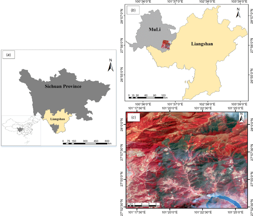
The research area was selected within localised burn extents of the 2020 MuLi Forest Fire, where time sequential multi-source remote sensing images were collected, as shown in Fig. 1. The geographical coordinates of MuLi County are (100.139859E, 28.942699N), encompassing a total area of 13,252 km2, with an administrative district boundary measuring 134.81 km. MuLi exhibits typical mountainous, hilly and canyon-like landforms, with three primary topographical features: northwestern mountainous terrain, southeastern middle-height mountain terrain and southwestern high-mountain terrain. According to meteorological data from the China Meteorological Administration (CMA), the county experiences distinct dry and wet seasons, with an annual average temperature of 14°C. The fire started at 19:30 hours on 28 March 2020, with the ignition point located at coordinates (101.379492E, 27.900137N). The prevailing wind directions were from the northeast and northwest, while the average wind speed ranged from 2.5 to 3.0 m s−1.
Preparation of the data
The present study incorporates various spatiotemporal factors influencing fire spread, encompassing wind speed, wind direction, distribution of vegetation, thermophysical parameters of vegetation and topographic conditions. The collected data include fire ignition points (fire ignition lines), a digital elevation model (DEM), wind speed and direction, and Sentinel-2A satellite images, as well as the vegetation map of China. Table 1 presents a summary of the data sources.
| Data type | Precision | Data source | |
|---|---|---|---|
| Digital elevation model | 10 m | United States Geological Survey | |
| Sentinel-2A | 10 m | United States Geological Survey | |
| Wind speed | 3 h | National Meteorological Information Center | |
| Wind direction | 3 h | National Meteorological Information Center | |
| Vegetation map of China | – | Resource and Environment Science and Data Center | |
| GLC_FCS30-2020 | 30 m | Aerospace Information Research Institute (AIR), Chinese Academy of Sciences (CAS) | |
| Google Digital Image | 2.39 m | China Meteorological Administration (CMA) |
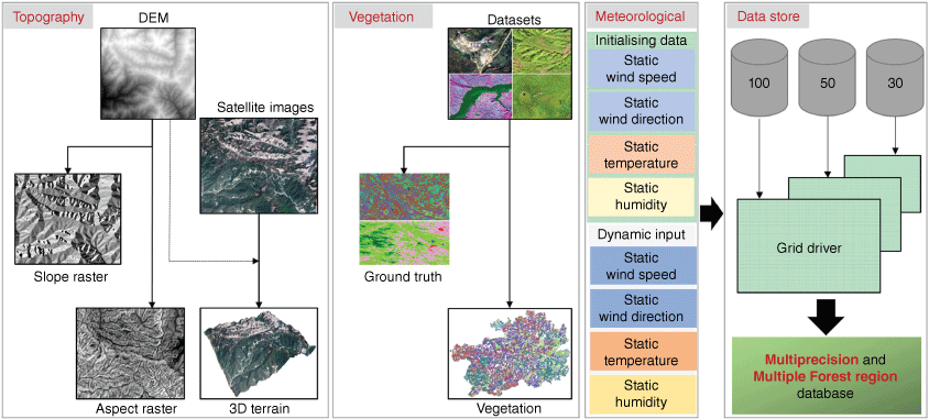
We use ArcGIS 10.1 software to conduct data manipulations and analyses for pre-processing purposes. The DEM is clipped to the study area boundary and converted into the raster data representing slope and aspect. The spatial distribution information of vegetation is derived by an instance segmentation method (Zhao et al. 2022) based on Sentinel-2A remote sensing images, aiming to assess the diversity of vegetation within the study area. Further, thermo-physical parameters of various vegetation fuels are obtained through systematic sampling and measurement. Dynamic meteorological data every 3 h from 29 to 31 March 2020 are collected within the study area to consider the influence of meteorological parameters. Finally, all the data are incorporated into the geospatial information database, defined as a ‘quartel grid’. The process of data preparation is schematically illustrated in Fig. 2.
Data preparation process. Topography encompasses slope and aspect; vegetation encompasses distribution and parameters; meteorological factors encompass wind speed, wind direction, temperature and humidity; the data store comprises two pivotal aspects: multi-precision and multiple forest regions.
Vegetation inversion
For the study area, we introduce multi-source and multi-temporal remote sensing images to construct comprehensive datasets for vegetation inversion. To establish ground truth, we adopt the vegetation map of China (1:1,000,000) (Wu et al. 2022), the Global Land Cover Product with Fine Classification System at 30 m for 2020 (GLC_FCS30-2020) (Meng et al. 2022), and up-to-date data from Google Digital Image. Subsequently, we utilise Labelme (Russell et al. 2008) to construct labels. The train and test datasets are constructed using Sentinel-2A remote images, encompassing infrared spectral bands across different seasons. Specifically, the vegetation map of China (1:1,000,000) and the GLC_FCS30-2020 provide information on vegetation types within various compartments, while Google Digital Image and labels offer the boundary delineations of vegetation. Moreover, we divide the built training and test dataset into three subsets: 70% for the training dataset, 25% for the test dataset and 5% for the validation dataset.
We obtain the spatial distribution information of vegetation by combining the maximum likelihood (ML) technique (Otukei and Blaschke 2010) and the Hybrid Task Cascade (HTC) algorithm (Chen et al. 2019). The ML technique is a non-linear supervised classification method based on Bayes’ theorem, which necessitates the derivation of prior probability and conditional probability density functions from provided training samples. The HTC algorithm is a multi-task and multi-stage hybrid cascade instance segmentation approach that enhances information flow by integrating cascaded stages and multi-tasking capabilities at each stage.
The ML method integrated within ArcGIS and the HTC model are utilised for vegetation inversion, with the fusion of results achieved by incorporating ground truth data and manual priors. Moreover, non-combustible objects such as rivers and villages are identified and categorised using the abovementioned approach to serve as natural barriers for fire spread within forested regions. These natural barriers are excluded from the outcomes to enhance the reliability of the inversion.
Fire spread models
The fire spread modelling incorporates the Rothermel (1972) and the Time-WZF rate models (Sun et al. 2021), considering the topographical slope factor in MuLi County. The study area is partitioned into a grid of square-shaped cells with uniform dimensions (i.e. sides measuring 30, 50 and 100 m). The ROS R is determined using Eqn 1 when slope ≤25° as recommended in the Rothermel model (1972):
where the reaction intensity IR (kJ m−2 min−1) represents the heat release per unit area of the fire front, ξ denotes the no-wind propagating flux ratio, Φs is a slope factor, Φw is the wind coefficient, ρb (kg m−3) is the oven-dry bulk density and Qig (kJ kg−1) is the heat required to ignite a unit weight of fuel. The wind coefficient ΦW is calculated using:
where
The slope factor ΦS is calculated according to Eqn 4:
where β is the filling rate, ϕ is the slope and σ is a function coefficient.
The ROS R is calculated according to Eqn 5 when 25°< slope ≤ 60° as recommended in the Time-WZF model (Sun et al. 2021):
where R0 is the initial ROS (m min−1), Kφ is the wind coefficient, Kθ is a terrain factor, Ks is the combustible index (obtained from a look-up table (Wang 1992)); Kr is the time correction coefficient, set to 0.04 as suggested in Rui et al. (2018); a = 0.03, b = 0.05, c = 0.01, d = 0.3; T is the temperature (°C), W is the wind level, Int a set integer, RH is the air humidity (%), v is the wind speed (m s−1), θ is the slope angle, and g is the direction of the hill (1 for uphill and −1 for downhill). The model takes into account the effects of combustibles, wind, temperature, humidity and slope on the ROS.
Beyond the two models above, there is scope for incorporating additional models. The selection of the most appropriate model at each simulation step depends on the precise conditions of applicability, including vegetation type, slope and wind speed. As pointed out previously, the Rothermel model is employed for a slope less than 25°, whereas the Time-WZF model is selected when the slope falls within the range of 25°–60°.
Time-adaptive cellular automata
The CA model used in each grid incorporates eight directions (east, west, south, north, southeast, southwest, northwest and northeast). The rule for fire propagation encompasses both the interior and exterior of the grid, as illustrated in Fig. 3. The state of cells either changes or remains constant according to the local evolution rules. The state of a cell at a discrete time step tstep is determined by whether the propagation displacement Lspread exceeds the cell size along the spread direction Lsize. The Lsize is calculated with the grid size L, Lsize = L/2 in east, west, south and north directions, in southeast, southwest, northwest and northeast directions. Two local evolution rules are taken into account as follows:
Fire propagation outside the grid and within the grid. Rule 1 corresponds to the outside grid, and Rule 2 to the grid inside.
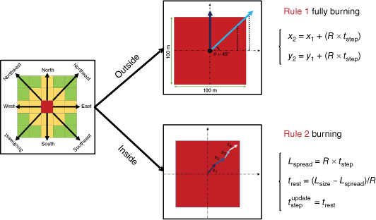
Rule 1: the fire spreads outside the grid if the propagation displacement Lspread exceeds the cell size along the spread direction Lsize. For the coordinate (x1, y1) of the fire point in current grid, the coordinate (x2, y2) in next grid during tstep can be calculated with:
where R is the ROS calculated by the model within the grid, and the coordinates (xi, yi) are the central coordinates of the grid considered as the coordinates of fire points. As illustrated in Fig. 3, when the propagation displacement Lspread along the northeastern direction exceeds the grid size Lsize = L/2, this indicates that the fire point has extended from the centre of one grid to the centre of an adjacent grid.
Rule 2: the fire spreads within the grid if the propagation displacement Lspread is smaller than the size of the cell along the spread direction Lsize. The propagation displacement Lspread is first calculated, followed by computation of the remaining time for spreading over the grid trest. Subsequently, the new time step is introduced into the spread calculation with Eqn 7 until the rule changes from 2 to 1:
where Lspread is the propagation displacement, Lsize is the grid size along the spread direction, trest is the extra time required to spread out of the current grid and is the new time step for a new simulation within the grid in this direction. According to Rule 2, the propagation displacement Lspread is evaluated against the grid size along the spread direction to adjust the duration within this grid, as shown in Fig. 3. This process continues until the fire point has successfully exceeded the current grid in the corresponding direction. During this phase, the coordinates of the fire point (xi, yi) are no longer fixed at the grid centre and change over time. Owing to the total simulating time ttotal being constant, Rule 2 may lead to inconsistent output times for simulation outcomes when compared with Rule 1. To address this discrepancy, the present study employs computational programming methodologies to ensure a consistent visualisation of simulation results across different time frames.
Assuming S is the state of the grid, according to Eqns 6 and 7, the transition from one state to another is calculated by:
where is the state of the grid (i, j) at the current moment, is that of the grid (i ± 1, j ± 1) at the next moment, is the ROS for each direction, which is approximately equal to in the ROS model within the grid approximately, Lsize is the grid size along the spread direction, Δt is the value of time step, t is the current time.
A critical condition judgment factor Cf reflects the relationship between propagation displacement and grid size within the current cell based on Eqn 8:
As time progresses discretely, the state of the neighbouring grid is determined by summing the state of the burning grid at the previous moment and the critical condition judgment factor Cf, adhering to the two local evolution rules. This process is depicted in Fig. 4. The critical condition judgment factor Cf represents the state of the current grid, defined as: Cf = 0, unburned; 0 < Cf < 1, burning, following Rule 2; and Cf ≥ 1, fully burned, following Rule 1. The variable S denotes the state of the adjacent grid at different time points, where S = 0 or S = 1 indicates that the adjacent grid state remains unburned, 1 < S < 2 indicates that the current grid has caused the adjacent grid to enter a burning state, and S > 2 indicates that the current grid has led the adjacent grid to reach a fully burned state. Wildfire propagation is often influenced by external factors such as fluctuating wind and active fire suppression efforts, resulting in slow propagation in the local direction. The proposed TCA model incorporates localised rules both within and outside the grid to achieve a controlled and deliberate fire spread in the local direction. The details of the input and output parameters of the TCA model are presented in Table 2.
Grid transition dynamics: fire propagation model, the adjacent grid states: unburned (a–b), burning (c) and fully burned (d). The centre S(i, j) represents the current grid with a fire point, surrounded by adjacent grids. The light green, orange and grey grids indicate the unburned, burning and fully burned states, respectively. The black bold arrows represent the transition of the grid state, while the red and grey arrows indicate the directions of wildfire spread.

Extraction of fireline
The location of the fireline is determined by employing the Normalized Burn Ratio (NBR) to identify burned areas through remote sensing images, as Epting et al. (2005) recommended.
where ρnir denotes the near-infrared band, ρswir represents the short-wave infrared band and the NBR index has a theoretical value ranging from −1 to 1.
The initial spatial information of the fireline is corrected using time series of remote sensing images through an adaptive simulation method, which involves integrating the extracted fireline coordinates with the proposed TCA model. Specifically, the NBR method is initially utilised to extract the coordinates of the fireline contour from t0 to tn−1, and subsequently calculate the average ROS in each direction, denoted R0, R1, R2, …, R7 based on the extracted information. Moreover, the fireline coordinates from t0 to tn−1 are used as the initial spatial information of fire spread at tn, and R0, R1, R2, …, R7 are adopted as the initial ROS instead of the results from the rate models. Finally, the proposed TCA model is integrated into a simulation system for wildfire propagation. The algorithm effectively addresses the challenges posed by non-linear factors such as dynamic wind and manual fire suppression.
Development of simulation system
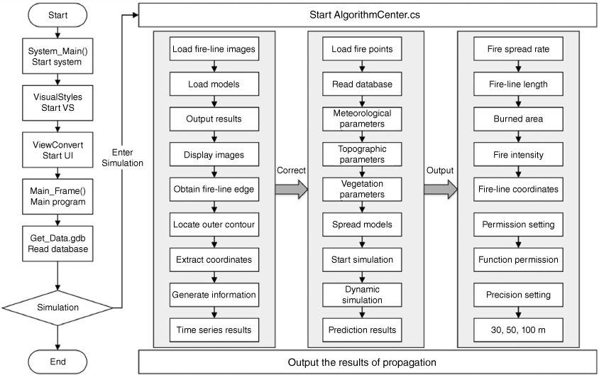
We evaluated the performance of the proposed method by developing a wildfire propagation simulation system based on ArcGIS Engine by C++, C# and XAML. A comprehensive static database that stores crucial topography, meteorology and vegetation parameters is incorporated into the system. The Rothermel model and Time-WZF model are embedded to calculate the ROS within the grid. The system integrates the proposed TCA model and utilises geographic information system (GIS) technology to achieve the three-dimensional and dynamic visualisation of fire propagation. Fig. 5 illustrates the technology pathway for the system.
The input conditions of the simulation system encompass the time step, total time and coordinates of a single fire point and fireline. The output parameters comprise the ROS, fireline length, burned area and fireline coordinates. Further, the fireline coordinates extracted from multi-source remote sensing images could be imported into the system as new initial spatial information to achieve adaptive fire spread simulation in subsequent time steps. The system also has a fireline identification module, which provides real-time spatial coordinates of firelines to simulate wildfire spread.
Results and discussion
Vegetation inversion results
By utilising the ML method integrated within ArcGIS and the HTC model, spatial distribution information on vegetation can be acquired with comprehensive datasets generated for training and testing purposes. The accuracy of predicting the probability of rivers reached 95%, while that for villages approached approximately 90% when compared with the GLC_FCS30-2020 and Google Earth System Digital Image. Moreover, the accuracy in predicting the probability of dominant vegetation was ~75% compared with ground truth labels. Importantly, inversion analysis provides more comprehensive information on the fire environment than previous research (Tavakol Sadrabadi and Innocente 2023; Xu et al. 2024), encompassing dominant vegetation, rivers and villages, as depicted in Fig. 6.
Vegetation inversion result: (a–b) are the inversion results with different grid sizes. The white areas indicate rivers and villages, while the other coloured areas represent vegetation.
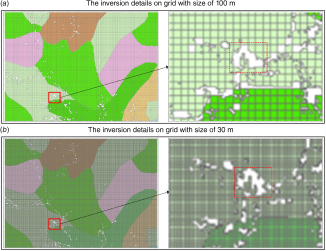
The inversion results provide crucial spatial distribution information on key ground objects, thereby highlighting the importance of fine-grained inversion in wildfire spread simulation.
Simulation results without and with the TCA model
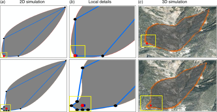
This section compares the simulation results without and with the proposed TCA model. The proposed model integrates two rules for higher and lower fire spread rates. The primary focus of the comparative analysis lies within the designated area highlighted in yellow shown in Fig. 7. The simulation results with the presented model effectively capture the gradual fire propagation trend in local regions. The proposed TCA model effectively addresses the limitations imposed by the time step and grid size, resulting in simulation outcomes that exhibit greater consistency with real wildfire environments. The local fire spread is specifically limited in the leeward direction of the fire front, thereby effectively preventing the fire front from surpassing its current grid within a given time step. Comparative analysis indicates that the proposed method effectively addresses the constraint imposed by grid size and time step on the spreading algorithm, thereby enabling a localised slow spreading simulation.
Simulation results without and with the proposed model, (a) 2D simulation, (b) Local details from (a), (c) 3D simulation. The first row represents the simulation result without the TCA model, whereas the second row corresponds to the simulation result with the TCA model. The red point denotes the ignition source, and the black points are generated by the spread of the wildfire. The blue line delineates the simulation result of the fire line. The yellow squares represent the local details of wildfire spread and the grey areas represent burned regions and the orange line is the wildfire boundary in 3D terrain.
Results of fireline extraction
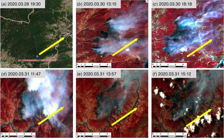
The time series of fire point distribution is derived from the GF4 and Sentinel 2A remote sensing images in the MuLi Forest Fire, as shown in Fig. 8. The ignition occurred at 19:30 hours on 28 March, as determined through investigation (Fig. 8a), with the initial coordinate of the fire point recorded as (101.379492E, 27.900137N). By 13:15 hours on 30 March, localised areas along the west started experiencing fire spread, contradicting the overall propagation trend of the fire (Fig. 8b), which can be attributed to local dynamic winds within the canyon. At 18:18 hours, there was a significant expansion in the fire-affected area (Fig. 8c). However, at 11:47 hours on 31 March, the fire intensified along the east (Fig. 8d), aligning with prevailing wind conditions. By 13:57 hours, the smoke plume from the fire displayed an upward trajectory (Fig. 8e), indicating a resurgence in fire intensity. Subsequently, at 15:12 hours, the fire spread towards the north–northeast direction with local weather conditions (Fig. 8f).
Forest fire monitoring in MuLi County based on GF-4 satellite data: (a–f) represent the fire spots at 19:30 hours on 28 March, 13:15 hours on 30 March, 18:18 hours on 30 March, 11:47 on 31 March, 13:57 hours on 31 March, and 15:12 hours on 31 March, respectively.
According to the analysis above, uncontrollable factors such as dynamic wind patterns and human intervention in fire suppression often pose significant challenges for quantifying localised fire spread outcomes during fire propagation, which presents substantial obstacles for fire propagation simulation. Therefore, the extraction of fireline coordinate information based on continuous time series remote sensing images (Fig. 9) and research on parameter initialisation for spreading simulations demonstrate significant importance.
Multi-source satellite remote sensing image extraction of the firelines: (a–c) represent the fire spots at 11:47 hours on 31 March, 13:57 hours on 31 March, and 15:12 hours on 31 March, respectively.
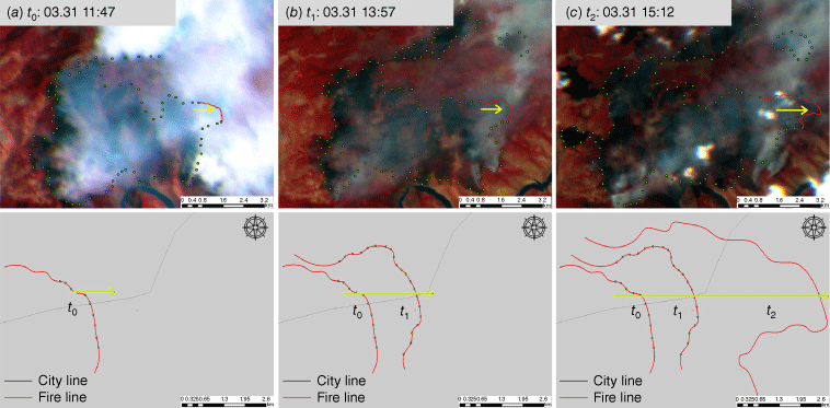
The location and shape of the fireline were extracted from multi-source remote sensing data (Fig. 9). The time series remote sensing images at 11:47, 13:57 and 15:12 hours on 31 March were selected based on the extracted fireline coordinates to achieve adaptive simulation. Considering the prevailing local weather conditions, particular attention was focused on the northeast fireline along the wind direction. The coordinates of the firelines at 11:47 hours (Fig. 9a) and 13:57 hours (Fig. 9b) were acquired using ArcGIS based on WGS_1984 UTM Zone 48N, as presented in Table 3. Specifically, the time denotes temporal data regarding distinct fire perimeters, the fire points represent a sequence of fire points along the current time on the fireline, direction indicates the primary direction of fire spread, and the coordinates provide the location information of the aforementioned fire points.
| Time (s) | Fire points | Direction | Coordinates (m) | |
|---|---|---|---|---|
| t0 | t0–1 | North | 151100.7619, 3097927.7381 | |
| t0–2 | Northeast | 151359.3825, 3097753.4856 | ||
| t0–3 | East | 151672.2631, 3097377.4037 | ||
| t1 | t1–1 | – | 151016.0951, 3098287.5722 | |
| t1–2 | North | 151132.3915, 3098374.1400 | ||
| t1–3 | – | 151281.1079, 3098418.2312 | ||
| t1–4 | – | 151456.7084, 3098435.8424 | ||
| t1–5 | – | 151592.0166, 3098518.8058 | ||
| t1–6 | – | 151753.9947, 3098555.1887 | ||
| t1–7 | Northeast | 151962.4567, 3098539.9271 | ||
| t1–8 | – | 152127.1761, 3098369.9600 | ||
| t1–9 | – | 152182.0241, 3098223.8979 | ||
| t1–10 | – | 152370.7645, 3098075.9051 | ||
| t1–11 | – | 152468.5928, 3097947.1883 | ||
| t1–12 | – | 152546.5481, 3097815.7274 | ||
| t1–13 | East | 152606.2621, 3097682.0542 | ||
| t1–14 | – | 152653.6741, 3097516.6865 |
Based on the results in Table 3, the ROS is calculated with the fire points coordinates at t0, including t0–1, t0–2 and t0–3, as well as the fire points at t1, namely t1–2, t1–7 and t1–13. The coordinates of fire points from t1–1 to t1–14 are also utilised as new fireline information for fire spread simulation at t2.
Simulation results based on parameters initialisation and TCA
Based on the above extracted fireline results, the fire spread trend observed in the remote sensing images from t1 to t2, combined with directional information provided by the TCA model show that the fire spread towards the north, northeast and east during this period. Consequently, three group fire points at t1 and t2 were selected to calculate the ROS in these directions.
After calculations, the spread distances in each direction are 805 m to the north, 991 m to the northeast and 934 m to the east. The rates of fire spread from t1 to t2 are determined as 0.103, 0.127 and 0.120 m s−1, respectively. To initialise the input parameters for simulation at t2, we assign the ROS as 0.103 m s−1 in the northern direction, 0.127 m s−1 in the northeast direction and 0.120 m s−1 in the eastern direction for all fire points ranging from t1–1 to t1–14. The initial fireline for simulation at t2 is selected based on the fire points within coordinates from t1–1 to t1–14, as presented in Table 4. This experiment successfully initialised the coordinates of the firelines and the ROS in each direction for simulating the fire spread from t1 to t2, overcoming the limitations associated with calculating ROS based on geographical parameters within a grid.
| Fire points | Direction | Coordinates (m) | Spread rate (m s−1) | |
|---|---|---|---|---|
| t1–1 | – | 151016.0951, 3098287.5722 | 0.103, 0.127, 0.120 | |
| t1–2 | North | 151132.3915, 3098374.1400 | 0.103, 0.127, 0.120 | |
| t1–3 | – | 151281.1079, 3098418.2312 | 0.103, 0.127, 0.120 | |
| t1–4 | – | 151456.7084, 3098435.8424 | 0.103, 0.127, 0.120 | |
| t1–5 | – | 151592.0166, 3098518.8058 | 0.103, 0.127, 0.120 | |
| t1–6 | – | 151753.9947, 3098555.1887 | 0.103, 0.127, 0.120 | |
| t1–7 | Northeast | 151962.4567, 3098539.9271 | 0.103, 0.127, 0.120 | |
| t1–8 | – | 152127.1761, 3098369.9600 | 0.103, 0.127, 0.120 | |
| t1–9 | – | 152182.0241, 3098223.8979 | 0.103, 0.127, 0.120 | |
| t1–10 | – | 152370.7645, 3098075.9051 | 0.103, 0.127, 0.120 | |
| t1–11 | – | 152468.5928, 3097947.1883 | 0.103, 0.127, 0.120 | |
| t1–12 | – | 152546.5481, 3097815.7274 | 0.103, 0.127, 0.120 | |
| t1–13 | East | 152606.2621, 3097682.0542 | 0.103, 0.127, 0.120 | |
| t1–14 | – | 152653.6741, 3097516.6865 | 0.103, 0.127, 0.120 |
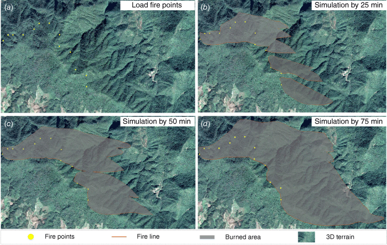
The dynamic simulation of wildfire spread is achieved through the initialisation of parameters and the application of the TCA model. The simulation of MuLi Forest Fire is presented over a duration of 75 min from t1 to t2, with a time step interval of 25 min. The primary wind direction is set as eastward. The coordinates of fire points and their corresponding spread rates in each direction are derived from Table 4. The simulation results are shown in Fig. 10. A comparison between the dynamic simulation results and multi-source remote sensing data, as presented in Fig. 9, indicates that the dynamic simulation accurately captures the observed trends in the burning area, with consistent shape changes reflecting those of the actual burning area. This consistency serves to validate the efficacy of the proposed method for simulating real wildfire events. According to Table 4, it is evident that the rates of spread in the eastern and northern directions are comparable. Consequently, the propagation outcomes should be similar within the same time step for both directions. However, observational data suggest a greater extent of eastward propagation compared with northward propagation. This behaviour may be attributed to the amalgamation of multiple simulation results along the wind direction, resulting in an expanded dispersion area. To accurately integrate simulation results from multiple fire points, this study calculates the propagation correction factor along the wind direction at t2 based on the firelines extracted from t0 to t1.
Dynamic simulation results by initialisation parameters. (a) Fire points by fireline. Simulation results (b) after 25 min, (c) after 50 min, (d) after 75 min. The simulated results coalesce on intersection.
For a qualitative assessment of the fire spread simulation outcomes, the simulation results were compared with the ground truth derived from time series remote sensing images, and the performance of the proposed method was evaluated based on the burned area and fireline length. As shown in Fig. 11, the overall spread trend, shape of the burned area and location of the fire front exhibit remarkable consistency with ground truth, thereby substantiating that time series remote sensing images demonstrated exceptional correction performance for the simulation. The effectiveness of the proposed TCA model is further confirmed by successfully simulating the gradual propagation scenario within a localised region.
Qualitative comparison of simulation results and real information. The grey area represents the simulation results, while the area bounded by the red line depicts the actual data. The period of the simulation is from t1 to t2.
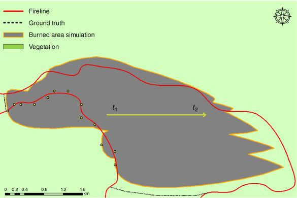
To further demonstrate the advantages of the proposed method, we conducted a comparative analysis between the simulation results of burned area and fireline length and their corresponding ground truth values, as presented in Table 5. The findings reveal that prediction accuracy of the burned area reached an impressive 92.2%, while the accuracy for fireline length prediction achieved 87.3%. The experimental results demonstrate that the proposed methodology effectively enhances the simulation precision and successfully addresses significant prediction errors caused by objective factors such as local dynamic wind patterns and human intervention in firefighting efforts.
Discussion
In the current scenario of frequent wildfires, the utilisation of multi-source remote sensing images plays a pivotal role in facilitating the simulation of wildfire spread. In this study, the primary aim was to utilise time series remote sensing images (Fig. 8) for extracting coordinates of fire points (Fig. 9), and to integrate the proposed TCA model for simulating wildfire spread in MuLi County. The ROS was calculated in each direction based on these extracted fire points (Table 3), and the combined fire points (Table 4) served as initial conditions for simulation in subsequent steps.
The imprecision of input parameters often leads to low accuracy in calculating ROS using the Rothermel model, mainly owing to the difficulty in quantifying dynamic wind and human intervention factors. In contrast, continuous time-series remote sensing can effectively mitigate these influences and provide more reliable initial parameters for the TCA model. Consequently, this approach serves as a valuable complement to the Rothermel model, particularly for accurately estimating ROS in complex fire environments. The aforementioned objective factors, such as dynamic wind and human intervention, often result in a significant reduction in the local rate of fire spread. This reduction may hinder the accurate characterisation of slow propagation in localised areas, particularly when applied to large grids over short periods. To address this issue, this study proposes a TCA model governed by two designed rules. The simulation results demonstrate a high degree of agreement with the observed fire spread patterns (Fig. 7). For the MuLi Forest Fire, the proposed method shows strong predictive capabilities. Qualitative results indicate that the overall spread trend, contours of the burned area and location of the fire front align well with ground truth observations (Fig. 11). Quantitatively, the prediction accuracy of the burned area reached 92.2%, while the prediction accuracy achieved for fireline length was 87.3% (Table 5). This study highlights challenges associated with small-scale wildfire spread while showcasing commendable performance in real wildfires. For large-scale wildfire spread simulation, data obtained from satellite imagery and Unmanned Aerial Vehicle (UAV) images can provide more precise parameters for the TCA model, suggesting its potential for future applications.
In terms of efficiency, the proposed method in this study demonstrates higher efficiency compared with other models. On one hand, Rule 1 shows comparable efficiency between TCA and CA. Despite a relatively lower efficiency of TCA compared with CA in Rule 2, TCA shows the capability to accurately simulate gradual spread within local regions without significantly reducing the overall efficiency of wildfire spread simulation. On the other hand, wildfire spread models that calculate ROS often require extensive geographical parameter inversion, resulting in low efficiency in ROS calculations. In contrast, utilising continuous time series satellite imagery to derive fire point coordinates and calculate average ROS circumvents inversion, thereby enhancing efficiency. Moreover, integrating UAV-based video instead of satellite imagery can significantly enhance parameter accuracy and overall efficiency.
A limitation of this study is the extended acquisition cycle of remote sensing imagery, which poses challenges for meeting real-time fire prevention and control requirements. Previous studies have highlighted the superior real-time capabilities of UAV imagery (De Vivo et al. 2021; Garcia et al. 2023; Ribeiro et al. 2023). Therefore, integrating the method proposed in the present paper with UAV monitoring could offer a viable solution for acquiring time series remote sensing images.
Conclusions
In this study, we propose an adaptive simulation method of wildfire propagation based on multi-source remote sensing images and cellular automata. The coordinates of the fireline are extracted to calculate the rate of spread (ROS) in each direction. The fireline coordinates and ROS are subsequently adopted as the initial conditions for simulation. A TCA model is proposed to address localised fire propagation with less uncertainty. It is demonstrated that the proposed adaptive simulation method can achieve fairly precise simulation results, while the presented TCA model has the capability to simulate fire spread with low ROS. The accurate prediction results obtained through the developed simulation software can serve as a powerful tool for wildland surface fire prevention and control.
The simulation of wildfire propagation poses a complex challenge in system engineering, with the accuracy of results closely tied to the accuracy of input parameters, spread models and correction data. To overcome the limitations of extended acquisition cycles and low resolution of remote sensing images, our forthcoming research will delve deeper into spatial error characterisation methods within grids and fireline identification models based on UAV images. The main focus of our efforts will be to enhance the precision of adaptive simulation outcomes to provide support for prevention measures against surface wildfires.
Nomenclature
| IR | reaction intensity (kJ m−2 min−1) |
| ΦS | slope factor (–) |
| ΦW | wind coefficient (–) |
| ρb | oven-dry bulk density (kg m−3) |
| Qig | heat of preignition (kJ kg−1) |
| C | function coefficient (–) |
| B | function coefficient (–) |
| E | function coefficient (–) |
| φ | slope (–) |
| R | speed of wildfire spread (m min−1) |
| R0 | initial speed of wildfire spread (m min−1) |
| Kφ | wind coefficient (–) |
| Kθ | terrain factor (–) |
| Ks | combustible index (–) |
| Kr | time correction coefficient (–) |
| a | constant (–) |
| b | constant (–) |
| c | constant (–) |
| d | constant (–) |
| T | temperature (°C) |
| W | wind level (–) |
| Int | set integer (–) |
| RH | air relative humidity (%) |
| v | wind speed (m s−1) |
| g | direction of hillslope (–) |
| tstep | time step (–) |
| update of time step under Rule 2 (–) | |
| Lspread | propagation displacement (m) |
| Lsize | the grid size along the spread direction [m] |
| trest | extra time required to diffuse out of the current grid (min) |
| S | the state of the grid [-] |
| state of the grid (–) | |
| ROS for each direction (m min−1) | |
| L | half size of the grid along the spread direction (m) |
| Δt | value of time step (–) |
| t | current time node (–) |
| Cf | critical condition judgment factor (–) |
| NBR | Normalized Burn Ratio (–) |
| tn | time node (–) |
Data availability
Data that support this study will be shared on reasonable request to the corresponding author.
Conflicts of interest
Dr Naian Liu is an Associate Editor of the International Journal of Wildland Fire. To mitigate this potential conflict of interest, he had no editor-level access to this paper during the peer review process. All authors hereby declare that they do not have any conflict of interest and have participated in (a) experimental design and analysis of the data; (b) drafting the article or revising it critically for important intellectual content; and (c) approval of the final version. This manuscript has not been submitted to, nor is it under review at, another journal or other publishing venue. The authors have no affiliation with any organisation with a direct or indirect financial interest in the subject matter discussed in the manuscript.
Declaration of funding
This research is sponsored by the National Key Research and Development Plan (No. 2022YFC3003000), and the National Natural Science Foundation of China (Nos 52321003, 51936011, and 52106186).
Acknowledgements
We thank the following people for help in the laboratory: Wei Gao and Hong Zhu for general advice and help.
References
Clarke KC, Brass JA, Riggan PJ (1994) A cellular automation model of wildfire propagation and extinction. Photogrammetric Engineering and Remote Sensing 60, 1355-1367.
| Google Scholar |
Crist MR (2023) Rethinking the focus on forest fires in federal wildland fire management: landscape patterns and trends of non-forest and forest burned area. Journal of Environmental Management 327, 116718.
| Crossref | Google Scholar | PubMed |
Cruz MG, Cheney NP, Gould JS, McCaw WL, Kilinc M, Sullivan AL (2021) An empirical-based model for predicting the forward spread rate of wildfires in eucalypt forests. International Journal of Wildland Fire 31, 81-95.
| Crossref | Google Scholar |
De Vivo F, Battipede M, Johnson E (2021) Infra-red line camera data-driven edge detector in UAV forest fire monitoring. Aerospace Science and Technology 111, 106574.
| Crossref | Google Scholar |
Epting J, Verbyla D, Sorbel B (2005) Evaluation of remotely sensed indices for assessing burn severity in interior Alaska using Landsat TM and ETM+. Remote Sensing of Environment 96, 328-339.
| Crossref | Google Scholar |
Garcia T, Ribeiro R, Bernardino A (2023) Wildfire aerial thermal image segmentation using unsupervised methods: a multilayer level set approach. International Journal of Wildland Fire 32, 435-447.
| Crossref | Google Scholar |
Gharakhanlou NM, Hooshangi N (2021) Dynamic simulation of fire propagation in forests and rangelands using a GIS-based cellular automata model. International Journal of Wildland Fire 30, 652-663.
| Crossref | Google Scholar |
Junpen A, Garivait S, Bonnet S, Pongpullponsak A (2013) Fire spread prediction for deciduous forest fires in northern Thailand. Science Asia 39, 535-545.
| Crossref | Google Scholar |
McNamee M, Meacham B, van Hees P, Bisby L, Chow WK, Coppalle A, Dobashi R, Dlugogorski B, Fahy R, Fleischmann C, Floyd J, Galea ER, Collner M, Hakkarainen T, Hamins A, Hu L, Johnson P, Karlsson B, Merci B, Ohmiya Y, Rein G, Trouve A, Wang Y, Weckman B (2019) IAFSS agenda 2030 for a fire safe world. Fire Safety Journal 110, 102889.
| Crossref | Google Scholar |
Meng Q, Huai Y, You J, Nie X (2023) Visualization of 3D forest fire spread based on the coupling of multiple weather factors. Computers & Graphics 110, 58-68.
| Crossref | Google Scholar |
Meng S, Pang Y, Huang C, Li Z (2022) Improved forest cover mapping by harmonizing multiple land cover products over China. GIScience & Remote Sensing 59, 1570-1597.
| Crossref | Google Scholar |
Mitchell JW (2023) Analysis of utility wildfire risk assessments and mitigations in California. Fire Safety Journal 140, 103879.
| Crossref | Google Scholar |
Noble IR, Gill AM, Bary GAV (1980) McArthur’s fire-danger meters expressed as equations. Australian Journal of Ecology 5, 201-203.
| Crossref | Google Scholar |
Otukei JR, Blaschke T (2010) Land cover change assessment using decision trees, support vector machines and maximum likelihood classification algorithms. International Journal of Applied Earth Observation and Geoinformation 12, S27-S31.
| Crossref | Google Scholar |
Ribeiro TF, Silva F, Moreira J, Costa RL (2023) Burned area semantic segmentation: a novel dataset and evaluation using convolutional networks. ISPRS Journal of Photogrammetry and Remote Sensing 202, 565-580.
| Crossref | Google Scholar |
Rui X, Hui S, Yu X, Zhang G, Wu B (2018) Forest fire spread simulation algorithm based on cellular automata. Natural Hazards 91, 309-319.
| Crossref | Google Scholar |
Russell BC, Torralba A, Murphy KP, Freeman WT (2008) LabelMe: a database and web-based tool for image annotation. International Journal of Computer Vision 77, 157-173.
| Crossref | Google Scholar |
Sohail A (2023) Genetic algorithms in the fields of artificial intelligence and data sciences. Annals of Data Science 10, 1007-1018.
| Crossref | Google Scholar |
Sun L, Xu C, He Y, Zhao Y, Xu Y, Rui X, Xu H (2021) Adaptive forest fire spread simulation algorithm based on cellular automata. Forest 12, 1431.
| Crossref | Google Scholar |
Tavakol Sadrabadi M, Innocente MS (2023) Vegetation cover type classification using cartographic data for prediction of wildfire behaviour. Fire 6, 76.
| Crossref | Google Scholar |
Wang Z (1992) Current forest fire danger rating system (CFFDRS). Fire Safety Science 1, 121-125.
| Google Scholar |
Woinarski JCZ, McCormack PC, McDonald J, Legge S, Garnett ST, Wintle B, Rumpff L (2023) Making choices: prioritising the protection of biodiversity in wildfires. International Journal of Wildland Fire 32, 1031-1038.
| Crossref | Google Scholar |
Wu Z, Wang B, Li M, Tian Y, Quan Y, Liu J (2022) Simulation of forest fire spread based on artificial intelligence. Ecological Indicators 136, 108653.
| Crossref | Google Scholar |
Xu F, Chen W, Xie R, Wu Y, Jiang D (2024) Vegetation classification and a biomass inversion model for wildfires in chongli based on remote sensing data. Fire 7, 58.
| Crossref | Google Scholar |
Zhao Z, Liu Y, Zhang G, Tang L, Hu X (2022) The winning solution to the iFLYTEK challenge 2021 cultivated land extraction from high-resolution remote sensing images. In ‘Proceedings of the 2022 14th International Conference on Advanced Computational Intelligence (ICACI)’, 15–17 July 2022, Wuhan, China. pp. 376–380. (IEEE)
Zheng Z, Huang W, Li S, Zeng Y (2017) Forest fire spread simulating model using cellular automaton with extreme learning machine. Ecological Modelling 348, 33-43.
| Crossref | Google Scholar |


