

Evaluation and comparison of simple empirical models for dead fuel moisture content
Jason J. Sharples A B C * , P. Jyoteeshkumar Reddy D , Victor Resco de Dios E F , Rachael H. Nolan C G , Matthias M. Boer C G and Ross A. Bradstock C H
A
B
C
D
E
F
G
H
Abstract
The moisture content of litter and woody debris is a key determinant of fire potential and fire behaviour. Obtaining reliable estimates of the moisture content of dead fine fuels (i.e. 1-h and 10-h fuels) is therefore a critical requirement for effective fire management.
We evaluated and compared the performance of five simple models for fuel moisture content. The models belong to two separate classes: (1) exponential functions of the vapour pressure deficit; and (2) affine functions of the (weighted) difference between air temperature and relative humidity.
Model performance is assessed using error and correlation statistics, calculated using cross validation, over four empirical datasets.
Overall, the best performing models were the relaxed and generalised models based on the weighted difference between temperature and relative humidity.
Simple functions of the difference between air temperature and relative humidity can perform as well as, if not better than exponential functions of vapour pressure deficit. However, it is important to note the limitations of all these models when applied to fuels with moisture contents <10%.
The moisture content of fine dead fuels and woody debris can be reliably estimated using simple models that are amenable to easy application.
Keywords: 10-h fuels, empirical modelling, fine dead fuels, fuel moisture content, fuel moisture index, relative humidity, temperature, vapour pressure deficit.
Introduction
The amount of moisture present in wildfire fuels has a profound effect on fire potential and fire behaviour. For example, Matthews (2009) determined that fire potential and rate of spread, as assessed by the McArthur Forest Fire Danger Rating System (McArthur 1967; Noble et al. 1980), varies approximately as the inverse square of fine fuel moisture content, assuming all other factors are held constant. Bradstock (2010) also noted that low fuel moisture content is one of the four factors required to sustain wildfire propagation. The moisture content of dead fine fuels; i.e. litter and woody debris consisting of elements whose diameters are less than about 20–25 mm, is particularly important in determining whether ignitions develop into wildfires, their consequent rate of spread, and other factors such as the likelihood of spotting, crown fire transition and extreme wildfire development (Viegas et al. 1992; Davies and Legg 2011; Slijepcevic et al. 2013; Sullivan and Matthews 2013; Cruz et al. 2015; Cawson et al. 2020; Abram et al. 2021; Masinda et al. 2021; Reddy et al. 2021; Sharples 2022; Lopes et al. 2023; Ma et al. 2023). Fuel moisture content subsequently affects broader management decisions such as identifying prescribed burning windows, assessing the potential for fire self-extinguishment, assigning readiness/warning levels, deployment of personnel, appliances and other firefighting resources, and public mandates (e.g. fire bans). It is also a key variable in other areas, such as in ecological management and research (Matthews 2013).
Assessing the moisture content of fine dead fuels to within a reasonable degree of accuracy is therefore a critical consideration in wildfire management and in other areas of environmental science and application. A model for dead fine fuel moisture should be able to provide reliably accurate estimates of fuel moisture content across a variety of relevant ecosystem types and should not be so complex that its use is impractical. A variety of empirical and mechanistic models that meet these criteria can be found in the literature; empirical models specifically developed to estimate fuel moisture content include those of McArthur (1967), Simard (1968) and Sneeuwjagt and Peet (1998), but many more have been developed as auxiliary models associated with models for rate of spread (e.g. see Cruz et al. 2015). Mechanistic, or process-based models, formally account for the most important physical processes driving changes in fuel moisture, such as heat and moisture fluxes within a fuel layer and their interaction with the atmosphere above, as well as with the soil below the fuel layer. Examples of mechanistic fuel moisture models include those of Fosberg (1975), Nelson (2000), Wittich (2005) and Matthews (2006). Further examples of fuel moisture models can be found in the literature reviews of Viney (1991) and Matthews (2013).
Resco de Dios et al. (2015) introduced a semi-mechanistic model (denoted mD) to estimate dead fuel moisture content (FMC) based on its inverse exponential relationship with vapour pressure deficit (VPD). The VPD is a key variable influencing the flux of moisture between fine dead fuels and the surrounding atmosphere, and hence FMC. Resco de Dios et al. (2015) also compared the performance of mD to several other models from the fuel moisture modelling literature, including those of Simard (1968), VanWagner (1972) and Nelson (1984), which are so widely used that they are often taken as a benchmark for model comparison (Sharples et al. 2009; Nieto et al. 2010; Resco de Dios et al. 2015). Resco de Dios et al. (2015) also considered the simple fuel moisture index (FMI) introduced by Sharples et al. (2009).
Resco de Dios et al. (2015) found that mD consistently outperformed the other models in terms of mean absolute error (MAE), mean bias error (MBE) and the Akaike Information Criterion (AIC). While the FMI exhibited a lower AIC than mD when consideration was restricted to low FMC values (<20 and <10%), it systematically underpredicted FMC over any moisture range, and always showed higher MAE and MBE. However, the FMI is a dimensionless index that should only be considered as an equivalent scale for FMC – its values do not necessarily directly equate with fuel moisture content of fine dead fuels. As such, a comparison of FMC model output with raw FMI values is not entirely appropriate. A more meaningful comparison would involve a transformation of FMI, which converts the dimensionless values into dead fuel moisture contents (with units of %). In their analyses, Sharples and McRae (2011) used a simple scalar transformation of the FMI, but inspection of the results of Resco de Dios et al. (2015) – particularly their fig. 5 – suggests that an affine transformation of FMI could potentially yield a more useful model for dead fuel moisture content.
In this manuscript, the utility of the FMI is re-examined. Specifically, the FMI is extended via a simple affine transformation and the output of the resulting FMC model evaluated using empirical data. The performance of the modified FMI model is also compared to that of mD and several other models that can be viewed as generalisations or variants of the FMI and/or mD models.
Materials and methods
Fuel moisture models
Five dead fine fuel moisture models are considered in this study. They are as follows.
The FMI developed by Sharples et al. (2009) is a dimensionless index defined as a simple affine transformation of the difference between air temperature T (°C) and relative humidity H (%).
The specific form of the index was based on the broad observation that T − H ≤ 40 over forested landscapes (except in rare cases). As such, the FMI is (mostly) positive and increases as FMC increases. It is important to note that FMI does not directly produce fuel moisture content values per se. Rather, it provides an equivalent measure of fuel moisture content (similar to how air pressure provides an equivalent scale for measuring altitude, for example).
The relaxed FMI is determined as an affine transformation of the FMI, defined by the model parameters a and b, which are determined empirically:
The parameters a and b have units of %, so that FMIrel produces direct estimates of dead fuel moisture content.
The generalised FMI is a linear model with T and H as the independent variables, defined by the (empirically determined) model parameters a, b, and c:
The generalised FMI can be realised as an extension of the FMI and the relaxed FMI, in which the equal weightings given to temperature and relative humidity are allowed to differ and are determined empirically. The generalised FMI provides direct estimates of fuel moisture content, given that the parameters a, b and c have been assigned appropriate units. Models for fine dead fuel moisture content of this form can already be found in the literature; for example, Fosberg (1978), Pook and Gill (1993), Cheney et al. (2012), and Cruz et al. (2015) all consider models that have the same form as FMIgen.
The mD model is developed based on the inverse exponential relationship between the vapour pressure deficit of air (VPD) and dead fine fuel moisture content (Resco de Dios et al. 2015). This model was calibrated using the fuel moisture data of the first 90 days of the year at an Australian site using non-linear least squares fitting (for further details refer to Resco de Dios et al. (2015)). The model takes the form:
where mmin and mmax are the minimum and maximum of the observed fuel moisture content data used to train the model, respectively, and k is a parameter that represents the rate of decay of fuel moisture content with increasing VPD.
The mgen model is based on the inverse exponential relationship proposed by the Resco de Dios et al. (2015) with the rigid model parameters defined by mmin and mmax replaced by the more general model parameters a and b, which are determined empirically. The model takes the form:
The five fuel moisture models can be grouped into two structural groups defined by their functional forms: the first group (FMI, FMIrel, FMIgen) will be referred to as the ‘FMI Group’ of models; and the second group (mD, mgen) will be referred to as the ‘Exponential Group’ of models.
Fuel moisture and weather data
In this study, all models were calibrated and validated using the FMC data of Resco de Dios et al. (2015) combined with additional data obtained from the ACT Parks and Conservation Service (ACT PCS). The FMC data of Resco de Dios et al. (2015) were obtained from 1.9 cm diameter dowels connected to sensors. Specifically, three dowels were placed 30 cm above the ground facing to the north. The ACT PCS data were obtained as the average of three fuel moisture stick readings from five different sites. The fuel sticks were 1.27 cm diameter dowel, manufactured to weigh exactly 100 g when oven dried. They were placed in shaded areas approximately 15–20 cm above representative fuels, which included woody debris of approximately the same diameter as the dowels (ACT PCS, unpubl. data). For the dataset of Resco de Dios et al. (2015), only days with less than 2 mm of rain were considered in their analysis. We maintain this convention, and to ensure consistency across the datasets, we filter the ACT PCS data in the same manner. Specifically, rain values were extracted from AWAP gridded data (0.05°) (Jones et al. 2009) for grid cells near the site locations, and fuel moisture content values from the ACT PCS dataset corresponding to days on which rain was less than 2 mm were included in the analyses. The process for excluding rain-affected days was based on rain recorded to 09:00, which is standard procedure in Australian. Further details of the data are in Table 1.
| Data source | Site name | No. of FMC observations on days with rain <2 mm | No. of rain days (≥2 mm) | Time period | FMC range (%) | |
|---|---|---|---|---|---|---|
| Elevation | Data collection frequency | |||||
| Vegetation type | ||||||
| Resco de Dios et al. (2015) (fuel moisture sensor) | Cumberland plains | 311 | 51 | 01/01/2013–31/12/2013 | 5.6–44.4 | |
| 25 m | Daily | |||||
| Eucalypt, Melaleuca | ||||||
| ACT Parks and Conservation Service (average of three fuel moisture sticks) | Brindabella | 66 | 8 | 15/02/2017–14/04/2020 | 3.3–33.0 | |
| 750 m | Fortnightly | |||||
| Dry eucalypt forest | ||||||
| Honeysuckle | 65 | 6 | 15/02/2017–15/042020 | 3.0–43.0 | ||
| 1065 m | Fortnightly | |||||
| Dry eucalypt forest | ||||||
| Smokers gap | 61 | 10 | 15/02/2017–15/04/2020 | 3.7–40.7 | ||
| 1230 m | Fortnightly | |||||
| Dry eucalypt forest | ||||||
| Black mountain | 27 | 3 | 14/01/2019–15/04/2020 | 4.0–17.7 | ||
| 800 m | Fortnightly | |||||
| Dry eucalypt forest | ||||||
| Mugga | 31 | 1 | 14/01/2019–15/04/2020 | 1.7–21.0 | ||
| 680 m | Fortnightly | |||||
| Dry eucalypt woodland |
The two sets of FMC data can also be in Fig. 1, where they are plotted against VPD and FMI. The ACT PCS data did not contain direct measurements of VPD, so VPD (kPa) was calculated from temperature (T, °C) and relative humidity (H, %) as follows (Monteith and Unsworth 1990; Nolan et al. 2016):
Observed FMC values (%) plotted against (a) VPD (kPa), and (b) FMI for the Resco de Dios et al. (2015) (red squares) and ACT PCS (blue circles) datasets.
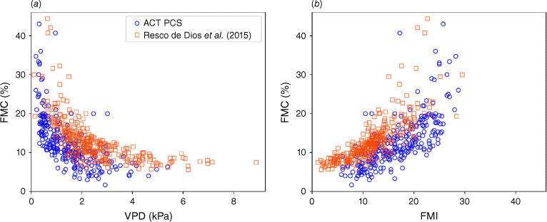
A discrepancy between the FMC data of Resco de Dios et al. (2015) and ACT PCS can be in Fig. 1, with the FMC values of Resco de Dios et al. (2015) offset from the ACT PCS values by about +5%. This discrepancy could be due to differences in the diameter of the dowels used as fuel sticks (12.7 mm for ACT PCS compared to 19.0 mm for Resco de Dios et al. 2015) and the height above ground the fuel sticks were placed (15–20 cm for ACT PCS compared to 30 cm for Resco de Dios et al. 2015). Microclimatic differences between the ACT PCS field sites and the site used by Resco de Dios et al. (2015) and differences in the sampling times could also account for the observed discrepancy. This discrepancy is disregarded in the analyses presented, but the issue is discussed further in a later section of the paper along with potential ramifications.
The models are calibrated and tested using four different datasets made up of fuel moisture content values and the corresponding weather data. Specifically, these datasets are as follows:
The set of all fuel moisture sensor data and associated weather variables used by Resco de Dios et al. (2015) combined with the set of fuel moisture content values and associated weather variables collected by ACT Parks and Conservation Service. This dataset comprises N1 = 561 elements and is denoted D1.
The subset of D1 consisting of N2 = 510 elements with fuel moisture content values below 20%, and denoted D2.
The subset of D1 consisting of N3 = 232 elements with fuel moisture content values above or equal to 10% and below 20%, and denoted D3.
The subset of D1 consisting of N3 = 187 elements with fuel moisture content values below 10%, and denoted D4.
Assessment of model performance
The predictive ability of the models was evaluated and compared through calculation of several performance statistics, similar to those considered by Resco de Dios et al. (2015). Specifically, the following quantities were considered: MBE, mean bias error; MAE, mean absolute error; MSE, mean square error; RMSE, root mean square error; B1, the slope of a linear regression model fitted to the estimated and observed data; B0, the intercept of a linear regression model fitted to the estimated and observed data; R2, squared correlation coefficient for the regression model fitted to the estimated and observed data; AIC, Akaike Information Criterion; and Dr, the refined Willmott’s index of agreement (Willmott et al. 2012; Legates and McCabe 2013).
The statistics were estimated using k-fold cross-validation (Geisser 1995). In k-fold cross-validation, each of the three datasets Dj (j = 1, 2, 3, 4) is randomly split into k disjoint subsets of approximately equal size. For each ℓ = 1, …, k, the models are calibrated using nonlinear regression on the set to determine the model parameters. The subset is then used as validation data to permit estimation of the correlation and error statistics mentioned above. In this study, the value k = 10 was chosen, and the entire 10-fold cross-validation process just described was replicated 10 times to produce 100 samples of the fitted model parameters and an estimate of the distribution of each of the performance statistics, which are reported in the next section. Unlike other validation techniques, k-fold cross validation utilises all the available data for training and testing the model by generating different folds.
The nonparametric permutation test (Singh et al. 2021) was used to assess the statistical significance of the differences in the mean of the performance statistics of different model pairings (see Supplementary Material Fig. S1).
Results
Model performance and intercomparison
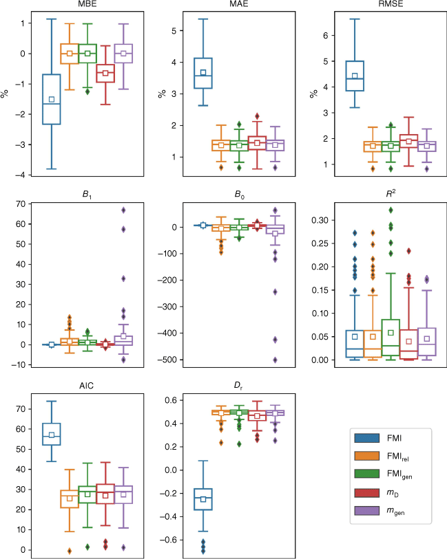
The error and correlation statistics obtained using dataset D1 are in Fig. 2, where the distributions of the various statistics are presented as box and whisker plots. The figure indicates the models that performed best overall were FMIrel, FMIgen, and mgen. These models clearly performed better than FMI and mD in terms of MBE, with FMIrel, FMIgen, and mgen all exhibiting approximately symmetric distributions centred near 0%, while FMI and mD registered mean MBE values of around −1 and +2%, respectively. The FMIrel, FMIgen and mgen models exhibited the lowest values of MAE and RMSE, while the mD model consistently exhibited the largest error statistics. The nonparametric permutation test (Table S1) indicated that the MAEs and RMSEs for FMIrel, FMIgen and mgen, were statistically significantly better than the other models. In the case of MAE, the FMIrel, FMIgen and mgen models all performed statistically significantly better than FMI and mD at the 0.05 significance level (Table S1).
Box and whisker plot of the performance statistics of all five models (blue = FMI, orange = FMIrel, green = FMIgen, red = mD, and violet = mgen) obtained using 10-fold cross-validation with dataset D1. The lower end and upper end of each box represents the 25th and 75th percentile values, respectively. The whiskers represent 1.5 times the respective interquartile (25th and 75th) range. The small boxes and lines represent the mean and median, respectively. Solid diamonds represent outliers.
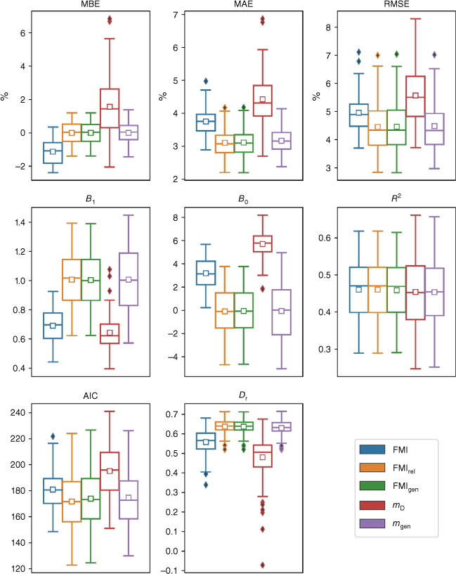
The distributions of the correlation statistics B1, B0 and R2 also indicated that the best performing models were FMIrel, FMIgen and mgen, with each exhibiting distributions of B1 and B0 with means and medians very close to 1 and 0, respectively. The FMI and mD models exhibited the worst performances in terms of B1 and B0, although it should be noted that this is not surprising for FMI, given that it is not intended to directly produce fuel moisture content values, as described above. These results for FMI are also consistent with those presented by Resco de Dios et al. (2015, fig. 5). The FMI Group of models exhibited slightly larger mean and median R2 values, but the differences weren’t statistically significant (Table S1).
The three models FMIrel, FMIgen and mgen have the greatest number of parameters, and so it is perhaps unsurprising that they produce the best error and correlation statistics. However, the AIC, which accounts for parametric dependence, also indicates that these three models performed the best, as Fig. 2 shows the mean and median AIC values for these three models were lowest. The refined index of agreement Dr also indicates that FMIrel, FMIgen and mgen were the best performing models. The worst performing models in terms of both AIC and Dr were mD and FMI, with FMIrel, FMIgen and mgen all producing significantly better AIC and Dr values than these two models (Table S1).
The results for the dataset D2, which focuses on fuel moisture content values below 20%, are shown in Fig. 3. In terms of MBE, the FMIrel, FMIgen and mgen models were again the best performing models, all exhibiting mean values very close to 0%, while FMI performed the worst with a mean negative bias of about −1.7%. FMIrel, FMIgen and mgen were also the best performing models in terms of MAE and RMSE, producing statistically significantly lower values than mD, which was the next best performing model (Table S1). In fact, the FMIgen model performed slightly better in terms of MAE, significantly better (at the 0.1 level) than mgen, but not significantly better than FMIgen. The FMIrel, FMIgen and mgen models also performed best overall in terms of the correlation statistics. They produced values of the slope B1 that were consistently the closest to unity and values of the intercept B0 consistently closest to zero. These models were closely followed by the next best performing model mD, which exhibited B1 values of around 0.8 and B0 values of around 1.0. The FMI model exhibited the worst performance in terms of B1 and B0, though again, these statistics are not that relevant for this model.
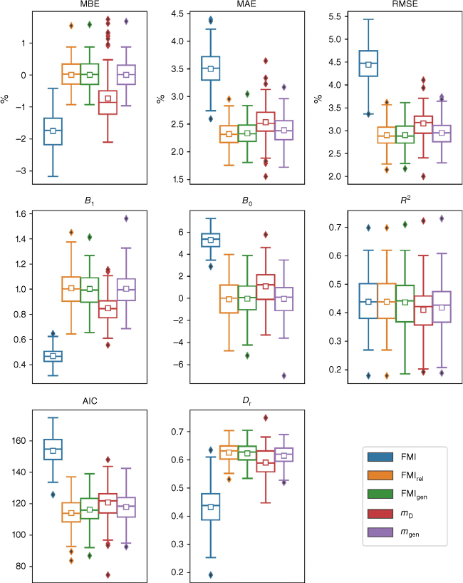
The FMI Group of models produced slightly higher R2 values than the Exponential Group of models, but the differences were only statistically significant for the mD model (Table S2). The FMIrel and FMIgen models also produced the lowest AIC values and highest Dr values. In terms of AIC, the FMIrel model performed the best. While FMIrel didn’t perform significantly better than FMIgen, it did perform significantly better (at the 0.05 level) than all the Exponential Group of models. The FMIgenmodel was the next best model in terms of AIC, though it didn’t perform significantly better than mgen. Similarly, the FMIrel model performed the best in terms of Dr. It significantly outperformed all the Exponential Group models (at the 0.05 level) but was not significantly better than FMIgen. The FMIgen model also performed significantly better than mD, but not significantly better than mgen.
The results for fuel moisture content values between 10 and 20%, belonging to the dataset D3, are shown in Fig. 4. Again, the FMIrel, FMIgen and mgen models exhibited the MBE values closest to 0%, while FMI performed the worst, with a mean negative bias of about −1.9%. In terms of MAE and RMSE there was no statistically significant difference between the FMIrel, FMIgen, mD and mgen models, but all were significantly (at the 0.05 level) better performing that FMI (see Supplementary Table S3). The FMIrel, FMIgen and mgen models also performed best overall in terms of the correlation statistics. They produced values of the slope B1 that were consistently the closest to unity and values of the intercept B0 consistently closest to zero. These models were closely followed by the next best performing model mD, which exhibited B1 values of around 0.75 and B0 values of around 3.0. There was no statistically significant difference in the R2 values for any of the models considered (Table S3).
In terms of AIC, the mD model performed significantly better than FMIgen and mgen at the 0.05 significance level and better that FMIrel at the 0.1 significance level. The FMIrel model also had a significantly lower AIC value than FMIgen and mgen at the 0.1 level (Table S3). The FMI model performed significantly worse than all the other models in terms of AIC. The FMIrel, FMIgen, mD and mgen models were also the best performing in terms of Dr. All of these models exhibited Dr values significantly higher than the FMI model, but not significantly different to each other.
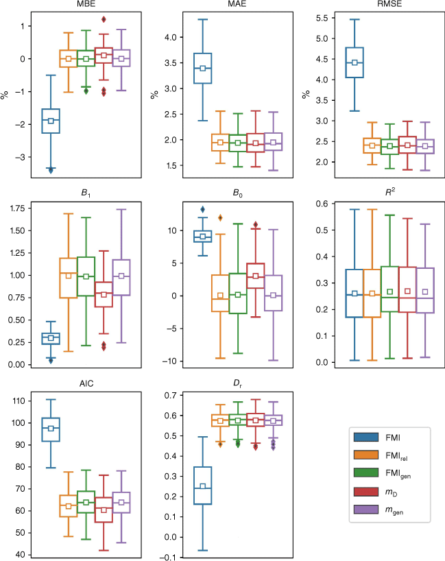
Fig. 5 confirms that FMIrel, FMIgen and mgen were also the best performing models when applied to the restricted dataset D4, which focuses on fuel moisture content values below 10%. These three models consistently exhibited smaller error statistics than the other models considered. In terms of MBE, each of these models produced roughly symmetric MBE distributions centred on zero. The mD model was the next best model in terms of MBE, displaying a slight negative bias, while FMI was the worst performing, exhibiting negative biases of −2%, or more. The FMI model also produced statistically significantly higher (at the 0.05 level) values of MAE and RMSE (Table S4). The mD model also produced significantly higher RMSE values than the three best performing models (at the 0.05 level). The MAE values for the mD model were only statistically significantly higher than those for the FMIrel and FMIgen models at the 0.1 level, and not significantly higher than the MAE values for the mgen model (Table S4).
The correlation statistics for the D4 dataset were problematic. The FMIrel, FMIgen and mgen models all produced a wide range of B1 and B0 values and the R2 values for all models were very low, with mean values of around 0.05 and even lower median values. There were no statistically significant differences in the R2 distributions for each of the models, except for FMIgen, which exhibited significantly higher R2 values than the mD model (at the 0.05 level). Overall, it was not possible to identify a best performing model from the correlation statistics.
The FMIrel model produced the most favourable AIC results; significantly better (at the 0.05 level) than those for the FMI, FMIgen and mgen models, but not significantly better than the mD model (Table S4). In terms of Dr, the FMIrel, FMIgen and mgen models gave the best results, with no statistically significant differences in model performance. These three models also had significantly higher Dr values than the mD model (at the 0.05 level). The AIC and Dr distributions for the FMI model were all statistically significantly worse (at the 0.05 level) than those of the other models (Table S4).
Distribution of model parameters
Fig. 6 shows the distributions of the various parameter values obtained from the 10 replications of 10-fold cross validation on each of the datasets D1, D2, D3 and D4, for each of the models considered (except FMI). Differences in the parameter estimates for each of the models can be seen, dependent upon whether the fuel moisture values were unconstrained, or constrained to be <20%, between 10 and 20%, or <10%. For the FMIrel model, when applied to the full dataset D1, the parameter a has a mean value of around 3.2. However, when applied to the restricted dataset D2, the parameter a has a larger value centred around 5.3, while for the further restricted dataset D4, the parameter a has an even larger value centred around 7.2. The largest values of the parameter a were found for the intermediate dataset D3. For this dataset, with fuel moisture varied between 10 and 20%, the parameter a assumed values of around 9.0. The parameter b varies in roughly the opposite manner with the largest values of around 0.69 found for the D1 dataset, smaller values of around 0.47 for the D2 dataset, values of around 0.3 for the D3 dataset and even smaller (near zero) values of around 0.04 for the D4 dataset.
Box and whisker plots for the estimated parameters of the respective models obtained using 10-fold cross-validation with each of the datasets (blue = D1 (all data), orange = D2 (FMC < 20%), green = D3 (10% ≤ FMC < 20%), red = D4 (FMC < 10%)). The lower end and upper end of each box represents the 25th and 75th percentile values, respectively. The whiskers represent 1.5 times the respective interquartile (25th and 75th) range. The small boxes and lines represent the mean and median, respectively. Solid diamonds represent outliers.
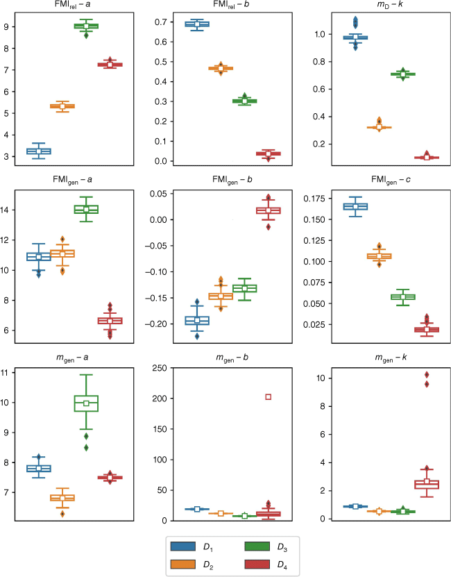
These parameter distributions indicate a reduction in the FMI-sensitivity of the FMIrel model as the FMC data is restricted below the 20 and 10% thresholds. For the full dataset D1, the variability in the FMC data is well-accounted for by FMI, while for the D2 dataset there is less ‘FMI signal’ in the data, though the FMIrel model still does a good job of predicting FMC, as has been shown. This trend continues through to the intermediate fuel moisture dataset D3, while for the D4 dataset there is minimal dependence on FMI, with the model dominated by the constant term a, which simply returns a value close to the mean FMC for D4.
This interpretation of the FMIrel parameters is supported by the distributions of the exponential parameter k in the mD model. For the dataset D1, the parameter k has values close to 1.0, larger that the values of k near 0.3 for the dataset D2, while for dataset D4 the parameter k assumes values of around 0.1. This indicates that FMC was most sensitive to VPD over the full dataset, less sensitive to VPD when FMC was restricted to <20% and least sensitive to VPD when FMC < 10%. These results can be explained through inspection of Fig. 1a, which shows a distinct ‘flattening’ of the relationship between FMC and VPD when FMC < 10%, indicating a lack of signal related to VPD in these data. A similar pattern can be seen in the relationship between FMCand FMI when FMC < 10% in Fig. 1b. The pattern of data in Fig. 1a also explains the distribution of the parameter k for the dataset D3, which is centred around 0.7, approximately halfway between the values for the D1 and D2 datasets.
The parameter distributions for the FMIgen model tell a similar story, with progressively weaker dependence of FMC on temperature and relative humidity (via parameters b and c, respectively) for the D2 and D3 datasets compared to that for D1. In contrast, however, the parameter a exhibited only slight differences in the values obtained from the D1 and D2 datasets, with values close to about 11.0 in both cases. For the D3 dataset, the constant parameter a exhibited higher values than for D1 and D2, consistent with the respective distributions for the a parameter in the FMIrel model. For D4, the parameter a exhibited values of around 6.6, which are not too dissimilar to the values found for parameter a in the FMIrel model. For D4, the b and c parameter values are closer to zero (each around 0.02), thus indicating a much lower sensitivity of FMC to temperature and relative humidity for data satisfying FMC < 10%. Indeed, the b parameter distribution for D4 includes many positive values, indicating that FMC increases with temperature, which is distinctly at odds with other results obtained here and the existing literature. This suggests that the models should be treated cautiously when applied to estimation of very low FMC values (i.e. FMC < 10%).
For the three-parameter mgen model, the exponential parameter k that is centred around 0.90 for the full dataset D1, compared to about 0.5 for the restricted dataset D2, were similar values to those found for the exponential parameters of the mD model (Table 2). For the dataset D3, however, the parameter k was lower than the values obtained for the mD model. Parameter a centred around 7.8 for the D1 dataset, compared to about 6.8 for D2 and about 10 for D3, while the parameter b had values of around 19.1 for D1, compared to about 12.2 for D2 and 6.9 for D3. For the D4 dataset, the a parameter had values of around 7.5, which are roughly comparable to those found for D1 and D2, but the values for parameter b and the exponential parameter k were vastly different. Values of parameter b centred around 200, but with some values (not shown) exceeding several thousand. Similarly, the exponential parameter k varied widely, with a mean of around 2.7 but with some values reaching as high as 10. Such high values of the exponential parameter again indicate a lack of signal relating to VPD in the D4 dataset. For FMC values below 10%, the exponential models essentially revert to the mean FMC.
| Model (parameters) | |||||
|---|---|---|---|---|---|
| Dataset | FMIrel (a, b) | FMIgen (a, b, c) | mD (k) | mgen (a, b, k) | |
| D1 | 3.238, 0.688 | 10.875, −0.193, 0.165 | 0.982 | 7.803, 19.110, 0.887 | |
| D2 | 5.321, 0.465 | 11.063, −0.146, 0.106 | 0.325 | 6.808, 12.245, 0.540 | |
| D3 | 9.000, 0.304 | 14.051, −0.132, 0.058 | 0.709 | 10.003, 6.897, 0.463 | |
| D4 | 7.244, 0.036 | 6.616, 0.017, 0.019 | 0.103 | 7.495, 202.348, 2.667 | |
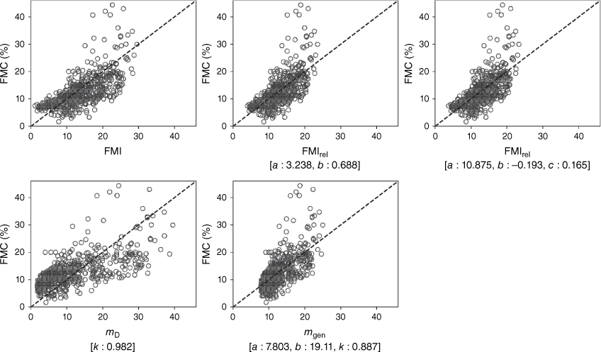
Table 2 provides a more precise summary of the estimated mean model parameter values for the distributions in Fig. 6, while Fig. 7 shows scatterplots of the FMC values against the various model predictions using the full dataset D1.
Scatter plots of observed FMC plotted against FMC predicted by each of the five models considered. The parameter values used to generate the plots are the mean values for the dataset D1 (see Table 2).
Discussion
Five relatively simple empirical models for estimating fuel moisture content have been evaluated and compared using four observational datasets. These models were based on the very simple fuel moisture index of Sharples et al. (2009) and the semi-mechanistic model of Resco de Dios et al. (2015). Overall, the analyses suggest that the FMI Group models FMIrel and FMIgen performed better than the Exponential Group of models (mD, mgen), though in most instances the performance of mgen was comparable (i.e. not statistically significantly different) to that of FMIrel and FMIgen. In contrast, FMIgen and FMIgen consistently performed significantly better than mD.
The models FMIgen and mgen are both defined by three parameters compared to FMIrel, which is defined by only two model parameters. So, this suggests that FMIrel should be favoured as the most parsimonious model. Furthermore, there was no discernible difference in the level of performance of FMIrel and FMIgen, across all the performance statistics. This suggests that the addition of an extra degree of freedom to the relaxed FMI model, to allow for different weightings of the influence of temperature and relative humidity, does not improve model performance. Indeed, the results indicate that the difference T − H, considered as a non-dimensional quantity, is a key predictor of dead fuel moisture content, but that it may lose its sensitivity when FMC < 10%. As has been previously noted (Sharples et al. 2009; Sharples and McRae 2011), operational personnel working on a fireground are routinely provided with basic information on air temperature and relative humidity. This information can be easily combined (via mental arithmetic) to calculate T − H, which then serves as a useful practical guide for estimating fuel moisture content under conditions commonly encountered in operational environments.
Some differences in the parameter estimates for each of the models were found, dependent upon whether the fuel moisture values were constrained to be <20%, between 10 and 20% or <10%. This indicates that the choice of model parameters should depend on the nature of the intended application. For example, if the intention is to assess fuel moisture content under wildfire conditions, then the parameter values derived using the restricted (e.g. FMC < 20%) datasets are more appropriate, while if the intention is to assess fuel moisture content under more benign conditions, then the parameter values derived from the full dataset are probably more appropriate. For more detailed consideration of prescribed burning thresholds, then the parameter values derived from the intermediate dataset D3 could be used. However, it is again noted that the results indicated that the models should be applied with some caution when predicting FMC values below 10%.
It is also important to note that the functional form of the models in the Exponential Group is such that these models saturate for high values of VPD. In fact, the models mD and mgen are, by definition, restricted to FMC > mmin, and FMC > a, respectively. This becomes an issue when attempting to predict critically low values of fuel moisture content, like those encountered during very hot and abnormally dry conditions, which are of key interest in the management of extreme wildfires (Sharples et al. 2016; Abram et al. 2021). For example, during the 2019–2020 Black Summer fire season in south-eastern Australia, some of the ACT sites recorded exceptionally low FMC values, with some as low as 1–2%. However, it should be noted that in the present study, the 10-fold cross validation procedure meant that mmin was essentially treated as an empirical parameter, whereas Resco de Dios et al. (2015) fixed mmin as the measured minimum FMC value over the whole dataset. Treating mmin as the measured minimum FMC should help with this issue, although none of the models considered performed particularly well when predicting FMC < 10%.
The models presented here have been developed and evaluated based on the observed fuel moisture content of fuels (sticks) with diameters of about 12–19 mm, which belong to the 10-h fuel size class (Deeming 1972). As such, the fuel moisture content of these fuels will take the order of about 10 h to equilibrate with the atmosphere; that is, changes in atmospheric conditions will not elicit an immediate response in fuel moisture content, and so care must be taken to accommodate this reality when applying the types of models considered here (Resco de Dios et al. 2015). Models in the FMI Group have also been used successfully to estimate fine dead fuel moisture content, which responds to atmospheric changes over a much shorter timeframe of about an hour (1-h fuel class). However, it may not be appropriate to apply the models derived here to predict 1-h fuel moisture content; to do so would require separate analyses, similar to those presented here, but based on 1-h fuels and weather data that has been recorded at sub-daily intervals.
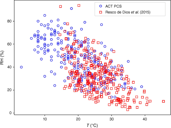
In the ‘Fuel moisture and weather data’ subsection, it was noted that the FMC values of Resco de Dios et al. (2015) were offset from the ACT PCS data by about +5%. This discrepancy could be due to differences in the dimensions and placement of the fuel sticks used to obtain the FMC data, differences in the microclimatic conditions of the field sites, differences in the sampling times and seasons, or a combination of these factors. For example, the data of Resco de Dios et al. (2015) was collected over the span of an entire year, and so included samples collected during winter and spring, whereas the ACT PCS data was only collected during late summer to mid-autumn. However, inspection of the associated temperature and relative humidity values for the two different datasets, depicted in Fig. 8, suggests that the climatic conditions were comparable; in fact, Fig. 8 indicates that, if anything, the ACT PCS sites experienced conditions that were overall cooler and moister than the site used by Resco de Dios et al. (2015). As such, the most likely reason for the discrepancy between the two data sets is differences in the dimensions and placement of the fuel sticks.
Observed relative humidity values (%) plotted against temperature (°C) for the Resco de Dios et al. (2015) (red squares) and ACT PCS (blue circles) datasets.
The main impact of the discrepancy between the two data sets was to obscure the FMI/VPD signal in the combined dataset when consideration was restricted to FMC < 10%. While it is possible to impose a systematic bias correction to remove some of the discrepancy between the two datasets, this was not pursued here. The effect that such a bias correction might have on the results presented here can be gauged by repeating the analyses with only one of the datasets considered. Thus, separate analyses (Figs S1–S5, Tables S5–S8) were performed using only the data of Resco de Dios et al. (2015). These analyses produced results that were similar to those presented above: when all the data of Resco de Dios et al. (2015) were considered, the FMIrel model performed the best overall – significantly better (at the 0.05 level) than FMI and mD, but not significantly better than FMIgen and mgen; when only FMC < 20% was considered, FMIrel was again the best performing model overall, performing significantly better (at the 0.05 level) than FMI, mgen and mD, though not significantly better than FMIgen; for fuel moisture between 10 and 20% FMIrel and FMIgen performed best overall, often significantly better than mD, but often not significantly better than mgen; while when FMC < 10% was considered, the FMIgen model performed statistically significantly better than the other four models across all of the error and correlation statistics. Using the measured minimum FMC as mmin, as proposed by Resco de Dios et al. (2015), instead of the estimated parameter a, could improve the predictive skill for mgen under low moisture. However, this would perhaps necessitate recalibration of the model when applied to new datasets. Overall, when only the FMC < 10% Resco de Dios et al. (2015) data is considered, the respective skill of the models considered was high compared to those trained on the combined dataset D4, although the models still exhibited considerably less skill compared to the FMC < 20% Resco de Dios et al. (2015) data. The distributions of the fitted model parameters also exhibited similar patterns of behaviour as seen for the combined dataset, except for those for the mgen model. In this case, the b and k parameters were far more constrained than they were for the combined dataset D3, though they still indicated a loss of sensitivity of FMC to VPD for lower FMC values.
Finally, it must be noted that the models presented here should only be applied in the absence of free moisture (e.g. dew or rainfall). Similarly, the models may not apply to estimation of moisture within thick fuel beds or near the bottom of fuel beds where fuel moisture can be influenced by soil moisture stores (Zhao et al. 2021). Similarly, other factors such as variation in solar radiation, topographic shading and wind exposure could also affect the moisture content of fuels in ways that are not accounted for in the models presented here (Nyman et al. 2015). Strictly speaking, the models presented here only apply to fuels that are sufficiently exposed to the atmosphere. It is possible, however, that the models presented here could be modified through incorporation of a variable such as a drought or soil moisture index to estimate average fuel moisture content throughout the fuel bed profile and to account for factors such as time since rain and rainfall amount (e.g. Goodrick 2002; Matthews 2006). This will be considered in future work.
Additional factors could also be incorporated through consideration of empirical datasets containing more detailed information on variables such as solar radiation, wind, litter depth, shrub layer characteristics and topographic setting (esp. topographic aspect). However, while inclusion of these additional factors would likely account for more of the variation in FMC data, it would also significantly compromise the parsimony of the models presented and their ease of use in field settings.
Conclusion
The ability to obtain reliable estimates of fuel moisture content of fine dead fuels is a key aspect of fire management. Fuel moisture content of 10-h fuels can be reliably estimated directly using either vapour pressure deficit, or by using the non-dimensional difference of air temperature and relative humidity, which acts as a proxy for VPD. In fact, simple affine models of T − H can perform just as well, if not better, than models that take the form of exponential functions of VPD.
Data availability
The data used in this study are available upon reasonable request from the authors.
Conflicts of interest
The first author, Jason J. Sharples, is an associate editor of the International Journal of Wildland Fire. To mitigate this potential conflict of interest, he was blinded from the peer review process and were not involved at any stage in the editing of this manuscript. There are no other conflicts of interest to declare.
Declaration of funding
This research was supported by funding from the NSW Government through the NSW Bushfire and Natural Hazards Research Centre.
Acknowledgements
The authors are grateful to the ACT Parks and Conservation Service for provision of fuel moisture content data and related information.
References
Abram NJ, Henley BJ, Gupta AS, Lippmann TJ, Clarke H, Dowdy AJ, Sharples JJ, Nolan RH, Zhang T, Wooster MJ, Wurtzel JB (2021) Connections of climate change and variability to large and extreme forest fires in southeast Australia. Communications Earth & Environment 2, 1-17.
| Crossref | Google Scholar |
Bradstock RA (2010) A biogeographic model of fire regimes in Australia: current and future implications. Global Ecology and Biogeography 19, 145-158.
| Crossref | Google Scholar |
Cawson JG, Nyman P, Schunk C, Sheridan GJ, Duff TJ, Gibos K, Bovill WD, Conedera M, Pezzatti GB, Menzel A (2020) Estimation of surface dead fine fuel moisture using automated fuel moisture sticks across a range of forests worldwide. International Journal of Wildland Fire 29, 548-559.
| Crossref | Google Scholar |
Cheney NP, Gould JS, McCaw WL, Anderson WR (2012) Predicting fire behaviour in dry eucalypt forest in southern Australia. Forest Ecology and Management 280, 120-131.
| Crossref | Google Scholar |
Davies GM, Legg CJ (2011) Fuel moisture thresholds in the flammability of Calluna vulgaris. Fire Technology 47, 421-436.
| Crossref | Google Scholar |
Goodrick SL (2002) Modification of the Fosberg fire weather index to include drought. International Journal of Wildland Fire 11, 205-211.
| Crossref | Google Scholar |
Jones DA, Wang W, Fawcett R (2009) High-quality spatial climate data-sets for Australia. Australian Meteorological and Oceanographic Journal 58, 233.
| Crossref | Google Scholar |
Legates DR, McCabe GJ (2013) A refined index of model performance: a rejoinder. International Journal of Climatology 33, 1053-1056.
| Crossref | Google Scholar |
Lopes S, Santos S, Rodrigues N, Pinho P, Viegas DX (2023) Modelling sorption processes of 10-h dead Pinus pinaster branches. International Journal of Wildland Fire 32, 903-912.
| Crossref | Google Scholar |
Ma W, Wilson C, Sharples JJ, Jovanoski Z (2023) Investigating the effect of fuel moisture and atmospheric instability on pyroCb occurrence over southeast Australia. Atmosphere 14, 1087.
| Crossref | Google Scholar |
Masinda MM, Li F, Liu Q, Sun L, Hu T (2021) Prediction model of moisture content of dead fine fuel in forest plantations on Maoer Mountain, Northeast China. Journal of Forestry Research 32, 2023-2035.
| Crossref | Google Scholar |
Matthews S (2006) A process-based model of fine fuel moisture. International Journal of Wildland Fire 15, 155-168.
| Crossref | Google Scholar |
Matthews S (2009) A comparison of fire danger rating systems for use in forests. Australian Meteorological and Oceanographic Journal 58, 41.
| Crossref | Google Scholar |
Matthews S (2013) Dead fuel moisture research: 1991–2012. International Journal of Wildland Fire 23, 78-92.
| Crossref | Google Scholar |
Nelson RM (1984) A method for describing equilibrium moisture content of forest fuels. Canadian Journal of Forest Research 14, 597-600.
| Crossref | Google Scholar |
Nelson RM (2000) Prediction of diurnal change in 10-h fuel stick moisture content. Canadian Journal of Forest Research 30, 1071-1087.
| Crossref | Google Scholar |
Nieto H, Aguado I, Chuvieco E, Sandholt I (2010) Dead fuel moisture estimation with MSG–SEVIRI data. Retrieval of meteorological data for the calculation of the equilibrium moisture content. Agricultural and Forest Meteorology 150, 861-870.
| Crossref | Google Scholar |
Noble IR, Gill AM, Bary GAV (1980) McArthur’s fire-danger meters expressed as equations. Australian Journal of Ecology 5, 201-203.
| Crossref | Google Scholar |
Nolan RH, Resco de Dios V, Boer MM, Caccamo G, Goulden ML, Bradstock RA (2016) Predicting dead fine fuel moisture at regional scales using vapour pressure deficit from MODIS and gridded weather data. Remote Sensing of Environment 174, 100-108.
| Crossref | Google Scholar |
Nyman P, Metzen D, Noske PJ, Lane PNJ, Sheridan GJ (2015) Quantifying the effects of topographic aspect on water content and temperature in fine surface fuel. International Journal of Wildland Fire 24, 1129-1142.
| Crossref | Google Scholar |
Pook EW, Gill AM (1993) Variation of live and dead fine fuel moisture in Pinus radiata plantations of the Australian-Capital-Territory. International Journal of Wildland Fire 3, 155-168.
| Crossref | Google Scholar |
Reddy PJ, Sharples JJ, Lewis SC, Perkins-Kirkpatrick SE (2021) Modulating influence of drought on the synergy between heatwaves and dead fine fuel moisture content of bushfire fuels in the Southeast Australian region. Weather and Climate Extremes 31, 100300.
| Crossref | Google Scholar |
Resco de Dios V, Fellows AW, Nolan RH, Boer MM, Bradstock RA, Domingo F, Goulden ML (2015) A semi-mechanistic model for predicting the moisture content of fine litter. Agricultural and Forest Meteorology 203, 64-73.
| Crossref | Google Scholar |
Sharples JJ (2022) A note on fire weather indices. International Journal of Wildland Fire 31, 728-734.
| Crossref | Google Scholar |
Sharples JJ, McRae RH (2011) Evaluation of a very simple model for predicting the moisture content of eucalypt litter. International Journal of Wildland Fire 20, 1000-1005.
| Crossref | Google Scholar |
Sharples JJ, McRae RHD, Weber RO, Gill AM (2009) A simple index for assessing fuel moisture content. Environmental Modelling and Software 24, 637-646.
| Crossref | Google Scholar |
Sharples JJ, Cary GJ, Fox-Hughes P, Mooney S, Evans JP, Fletcher MS, Fromm M, Grierson PF, McRae RHD, Baker P (2016) Natural hazards in Australia: extreme bushfire. Climatic Change 139, 85-99.
| Crossref | Google Scholar |
Singh J, Ashfaq M, Skinner CB, Anderson WB, Singh D (2021) Amplified risk of spatially compounding droughts during co-occurrences of modes of natural ocean variability. npj Climate and Atmospheric Science 4, 7.
| Crossref | Google Scholar |
Slijepcevic A, Anderson WR, Matthews S (2013) Testing existing models for predicting hourly variation in fine fuel moisture in eucalypt forests. Forest Ecology and Management 306, 202-215.
| Crossref | Google Scholar |
Sullivan AL, Matthews S (2013) Determining landscape fine fuel moisture content of the Kilmore East ‘Black Saturday’wildfire using spatially-extended point-based models. Environmental Modelling and Software 40, 98-108.
| Crossref | Google Scholar |
Viegas DX, Viegas MTSP, Ferreira AD (1992) Moisture content of fine forest fuels and fire occurrence in central Portugal. International Journal of Wildland Fire 2, 69-86.
| Crossref | Google Scholar |
Viney N (1991) A review of fine fuel moisture modelling. International Journal of Wildland Fire 1, 215-234.
| Crossref | Google Scholar |
Willmott CJ, Robeson SM, Matsuura K (2012) A refined index of model performance. International Journal of Climatology 32, 2088-2094.
| Crossref | Google Scholar |
Wittich KP (2005) A single-layer litter-moisture model for estimating forest-fire danger. Meteorologische Zeitschrift 14, 157-164.
| Crossref | Google Scholar |
Zhao L, Yebra M, van Dijk AI, Cary GJ, Matthews S, Sheridan G (2021) The influence of soil moisture on surface and sub-surface litter fuel moisture simulation at five Australian sites. Agricultural and Forest Meteorology 298–299, 108282.
| Crossref | Google Scholar |