Evaluation of seasonal teleconnections to remote drivers of Australian rainfall in CMIP5 and CMIP6 models
Christine Chung A * , Ghyslaine Boschat A , Andréa Taschetto
  B , Sugata Narsey A , Shayne McGregor C , Agus Santoso B and François Delage A
A Bureau of Meteorology, 700 Collins Street, Docklands, Melbourne, Vic. 3008, Australia.
B Climate Change Research Centre, University of New South Wales, Sydney, NSW 2052, Australia.
C School of Earth, Atmosphere and Environment, Monash University, Clayton, Vic. 3800, Australia.
Abstract
This study describes how coupled climate models participating in the sixth phase of the Coupled Model Intercomparison Project (CMIP6) simulate the primary climate drivers that affect Australian climate, and their seasonal relationship to Australian rainfall, namely the El Niño–Southern Oscillation (ENSO), the Indian Ocean Dipole (IOD) and the Southern Annular Mode (SAM). As results from the earlier generation of models (CMIP5) are still in use, the CMIP6 multi-model mean teleconnections between climate drivers and seasonal Australian rainfall are compared to CMIP5. Collectively, an improvement is found in CMIP6 relative to CMIP5 in the representation of the relationship between ENSO and IOD events and Australia’s springtime rainfall. Overall, CMIP6 models are also able to reproduce the asymmetric relationship between ENSO and eastern Australian rainfall, which exhibits a more robust signal during La Niña than during El Niño years. Both CMIP5 and CMIP6 models are also generally able to capture the stronger relationship between Central Pacific La Niñas, compared to Eastern Pacific La Niñas. However, the large spread in model-to-model behaviour, and among ensemble members, remains a source of uncertainty. Although CMIP6 models have improved in their representation of SAM variability, the simulated relationship between SAM and Australian rainfall has not materially improved. Additionally, this study is accompanied by an extensive Appendix in which each model’s ENSO, IOD and SAM seasonal teleconnection patterns to rainfall are presented and ranked.
Keywords: climate drivers, climate models, CMIP, ENSO, IOD, model evaluation, SAM, seasonal rainfall.
1Introduction
The sixth phase of the Coupled Model Intercomparison Project (CMIP6; Eyring et al. 2016) comprises over 100 models from modelling centres around the world and provides a comprehensive resource for the study of climate variability and change under a range of possible future scenarios. Climate models continue to improve in their representation of climate processes that critically affect aspects of life in Australia. How they are simulated in climate models matters deeply for informing users of climate change information, including efforts to downscale global climate model output to regional scales. This study evaluates the progress made in the most recent instalment of CMIP models, with a focus on how well they simulate the climate drivers most pertinent to Australia’s climate: the El Niño–Southern Oscillation (ENSO), the Indian Ocean Dipole (IOD) and the Southern Annular Mode (SAM).
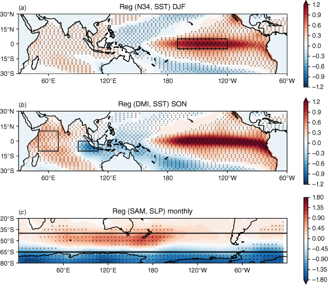
These three phenomena arise from processes originating in the atmosphere and ocean basins surrounding the Australian continent, and significantly influence regional rainfall variability and extremes on seasonal to interannual timescales (e.g. Risbey et al. 2009). From the tropical Pacific, ENSO (see Wang et al. 2017a and references therein) is a 3–7-year oscillation between El Niño (warm) and La Niña (cool) phases, in which warm and cool refer to sea surface temperature (SST) anomalies in the central to eastern equatorial Pacific (Fig. 1a). El Niño years are typically, though not always, associated with warm and dry conditions across northern and eastern Australia, and La Niña years are associated with cooler, wetter conditions (e.g. Risbey et al. 2009; Cai et al. 2010; Chung and Power 2017; Santoso et al. 2019; Taschetto et al. 2020). The IOD (Saji et al. 1999; Webster et al. 1999) is positive (negative) when the western Indian Ocean is anomalously warm (cool), and the eastern Indian Ocean is anomalously cool (warm) (Fig. 1b). During austral winter and spring, positive (negative) IOD events are typically associated with dry (wet) conditions across western, southern and south-eastern Australia (e.g. Ashok et al. 2003; Ummenhofer et al. 2009, 2011; Pepler et al. 2014; King et al. 2020; Liguori et al. 2022). Finally, the SAM is the leading mode of atmospheric variability in the southern hemisphere extratropics and describes the north–south expansion and contraction of the westerly wind belt around Antarctica (Gong and Wang 1999; Limpasuvan and Hartmann 1999; Marshall 2003; Fogt and Marshall 2020). Positive SAM phases are characterised by stronger westerlies, which are contracted towards higher latitudes and are associated with stronger storm tracks (Fig. 1c). These are associated with increased rainfall over eastern Australia in summer and winter, and decreased rainfall over southern Australia during winter (Hendon et al. 2007; Meneghini et al. 2007). Opposite conditions are observed during negative SAM phases.
(a) Observed Niño 3.4 index (averaged over box shown) regressed against the tropical Indo-Pacific SSTs for December–February (DJF). (b) Observed Dipole Mode Index (DMI; difference between east and west boxes shown) regressed against the tropical Indo-Pacific SSTs for SON. (c) Observed SAM index (difference between the sea level pressure zonally averaged along 40 and 65°S latitudes indicated by black lines) regressed against sea level pressure for SON. Panels (a) and (b) span 1950–2005 and panel (c) spans 1957–2005. Stippling indicates where regression is significant at the 95% level based on a t-test.
The teleconnections between ENSO and IOD to Australian rainfall are complex. In recent years, ENSO events have been sub-classified into Central Pacific (CP) or Eastern Pacific (EP) events (Kug et al. 2009; Capotondi et al. 2015) as the SST anomalies during these are often largest in the central or eastern Pacific. These distinct anomaly patterns generate different rainfall responses over Australia, with CP El Niños causing significantly drier conditions than EP El Niños (e.g. Taschetto et al. 2010; Yeh et al. 2018; Santoso et al. 2019; Ma et al. 2022). Additionally, there is an asymmetry, or non-linearity in the strength of ENSO events, with El Niño events being stronger than La Niña events, particularly in the eastern Pacific (e.g. Burgers and Stephenson 1999). The Australian rainfall response to El Niño and La Niña events, and positive and negative IOD events, is also asymmetric. La Niña events tend to generate larger rainfall anomalies than El Niño events (e.g. Cai et al. 2010, 2012; King et al. 2014; Chung and Power 2017; Taschetto et al. 2020), as do positive IOD (pIOD) events compared with negative IOD (nIOD) events (e.g. Cai et al. 2012). An added complexity is that ENSO and IOD often co-vary, with El Niño often co-occurring with pIOD and La Niña with nIOD, and so disentangling the impacts of the two on Australian rainfall variability is not straightforward (e.g. Ashok et al. 2003; Ummenhofer et al. 2015; Liguori et al. 2022). ENSO can also influence the phase of SAM, with El Niño acting as a precursor to negative SAM and La Niña preceding positive SAM, though the SAM response to ENSO usually lags by approximately one season (e.g. Dätwyler et al. 2020). The ENSO–SAM relationship has been poorly simulated in previous CMIP models due to inaccuracies in the simulation of the ENSO seasonal cycle (e.g. Lim et al. 2016).
As well as driving climate variability on seasonal to interannual timescales, ENSO, IOD, SAM and their interactions also strongly modulate the risk of climate extremes such as heat waves, floods and droughts. During the recent summer of 2019–20, eastern Australia sustained severe drought and widespread bushfires which have been linked to pIOD, a strong negative SAM and to a less extent to a CP El Niño (Lim et al. 2019; Wang and Cai 2020). Following this, three consecutive La Niñas and nIOD years preceded widespread flooding across many of the same regions. Recent studies (e.g. Holgate et al. 2022) have examined how the various phases of ENSO, IOD and SAM can affect rainfall-generating processes over eastern Australia. With these swings in climate drivers occurring atop a long-term warming trend, it is crucial that climate models are able to accurately simulate them in order to produce better-constrained projections to aid mitigation and adaptation efforts.
Recent studies (Grose et al. 2020; McKenna et al. 2020; Di Virgilio et al. 2022) have provided an overview of ENSO, IOD and SAM representation in CMIP6 models. We expand on these by discussing two aspects of this representation and how they compare to CMIP5 models. Firstly, we report on how well the large-scale climate drivers themselves are simulated using standard metrics by synthesising results of previous studies. Secondly, we evaluate how well the models simulate the teleconnections between these drivers and regional rainfall and climate. For ENSO, we address the nuances discussed above, including evaluation of models’ ability to reproduce the observed El Niño–La Niña asymmetry, CP and EP ENSO events and their respective teleconnections. We briefly examine pIOD–nIOD asymmetry; however, due to the co-variability between ENSO and IOD, the impacts of the two drivers are difficult to disentangle. We also briefly compare the observed historical trends in the climate drivers to those in CMIP5 and CMIP6 models.
Accurately simulating historical variability of these drivers and reproducing their regional teleconnections provide one way of assessing the performance and suitability of global climate models for selection in downscaling activities. Grose et al. (2023) evaluated CMIP6 models for selection in regional downscaling, selecting seven models chosen for their accuracy in simulating historical climate, as well as their ability to represent a range of possible climate futures (Grose et al. 2023). This evaluation complements such studies by further investigating the representation of the climate drivers and their regional teleconnections. Given that changes to climate drivers under global warming are a significant contributor to broader changes in climate, it is important to understand which models capture these drivers well. By contrast, those models that poorly represent climate drivers should be used with more caution when looking at their projections of climate change.
2Data and methods
In the teleconnection maps presented in this study, we analyse output from 58 CMIP6 and 42 CMIP5 models, using the first ensemble member from each model. In Sections 3–5, we also present ensemble spread for CMIP6 models that have more than one member (34 models with 3–49 members). Output from the historical scenario is analysed, spanning 1950–2005 for CMIP5 and CMIP6. Under the historical scenario, observed greenhouse gas, ozone and aerosol forcings are used in the models in order to replicate the observed climate of the 20th century as closely as possible (Taylor et al. 2012; Eyring et al. 2016). Modelled outputs are compared to 1950–2020 Australian rainfall observations from the Australian Gridded Climate Data (AGCD; Evans et al. 2020). All rainfall data are regridded to a 1.5 × 1.5° resolution.
The ENSO and IOD strength are measured using the Niño 3.4 and Dipole Mode Indices (DMI; Saji et al. 1999) respectively. The Niño 3.4 index is defined to be monthly SST anomalies in the central equatorial Pacific region (5°S–5°N, 170–120°W) and the DMI is the SST gradient between the western equatorial (50–70°E and 10°S–10°N) and south-eastern equatorial (90–110°E and 10°S–0°) Indian Ocean. Observed SSTs (1950–2020) are taken from HadISST (Rayner et al. 2003). The CP and EP ENSO indices are calculated following Sullivan et al. (2016), using standardised Niño3 (5°S–5°N, 150–90°W) and Niño4 (5°S–5°N, 160°E–150°W) indices (see Section 3.2.3 for details). To calculate the SAM index, we use the difference in zonal mean sea level pressure between 65 and 40°S (Gong and Wang 1999; Marshall 2003). Observed 1957–2020 SLP values are taken from station-based observations.1 All variables in this study (except when calculating long-term trends in Section 6) are quadratically detrended.
In the following sections, evaluations of ENSO, IOD and SAM metrics and teleconnections are presented for the CMIP6 multi-model means (MMMs), while noting that in some seasons there is a large inter-model spread. Model-by-model results are shown in the Appendix.
3ENSO and its impact on Australian rainfall
In this section, we first present a literature review of studies that have evaluated CMIP6 models’ skill in simulating ENSO variability, including their ability to simulate CP and EP ENSO events (Section 3.1). In Section 3.2, we evaluate the simulated teleconnections between ENSO and seasonal Australian rainfall for (i) all ENSO events, (ii) positive and negative Niño3.4 years separately and (iii) CP and EP El Niño and La Niña events separately.
3.1 Evaluation of ENSO metrics
The simulation of ENSO is closely linked to the dynamics and mean state of the tropical Pacific. In CMIP6, the MMM simulation of some aspects of the mean state of the tropical Pacific has improved compared to previous generations of climate models (Grose et al. 2020; McKenna et al. 2020). One significant improvement is in the common ‘cold tongue bias’, which is the tendency of many models to simulate an excessively cold ‘cold tongue’ in the equatorial Pacific that extends too far westwards (e.g. Li and Xie 2014). The cold tongue bias is related to many other tropical Pacific model biases, including spatial biases in the simulation of ENSO (e.g. Jiang et al. 2021), inaccurate forecasts of ENSO amplitude and duration (e.g. Kim et al. 2017; Wu et al. 2022) and spatial biases in ENSO teleconnections to Australian rainfall (Cai et al. 2011). Grose et al. (2020) found that the westward extension of the cold tongue is reduced by approximately 9° longitude in the CMIP6 MMM compared to the CMIP5 MMM.
The reduction in cold tongue bias has contributed to improvements in several aspects of ENSO representation, including its teleconnections. For example, Jourdain et al. (2013) reported an improvement in Australian monsoon response to ENSO from CMIP3 to CMIP5 models, and also noted that the strength of the Australian monsoon–ENSO teleconnection in most climate models depends on the strength of the simulated ENSO, which in turn is affected by cold tongue bias. A recent comparison of ENSO in CMIP5 and CMIP6 was conducted using a range of 24 metrics spanning, for example, spatial pattern, duration, global teleconnections and SST–wind feedbacks (Planton et al. 2021). This study found significant improvements in CMIP6 across eight metrics including spatial pattern and global teleconnections, and the simulation of ENSO diversity. Only one metric was significantly degraded compared to CMIP5, related to feedback between subsurface temperatures and SSTs in the eastern equatorial Pacific. The other metrics remained unchanged.
The ability to simulate CP and EP El Niños is important, as both flavours have been shown to have distinct impacts, particularly on Australian rainfall (e.g. Taschetto and England 2009; Santoso et al. 2019; Ma et al. 2022). Previous generations of models struggled to simulate two distinct regions of equatorial SST warming, with most favouring warming along the eastern Pacific (Taschetto et al. 2014; Feng et al. 2020). The CMIP6 models are able to better simulate CP El Niños (Planton et al. 2021; Hou and Tang 2022).
However, some other aspects of ENSO have not improved significantly. For example, some models underestimate ENSO seasonality and simulate a longer-than-observed life cycle (Taschetto et al. 2014, see their fig. 10 and 11), which results in persistent teleconnections at the tails of ENSO events (Jourdain et al. 2013). Also, one-third of CMIP5 models simulate the mature phase of ENSO to be outside the observed November–January window (Taschetto et al. 2014). This has not improved in CMIP6 (McKenna et al. 2020). The ENSO asymmetry and nonlinearity in the eastern Pacific remain underestimated (McKenna et al. 2020; Zhao and Sun 2022). The CMIP6 models also tend to overestimate the year-to-year variability along the western and central equatorial Pacific, leading to an overestimation of ENSO variability across most of the equatorial Pacific (McKenna et al. 2020).
It is also important to note that the tropical ocean basins do not operate in isolation. For instance, biases in the representation of the IOD are related to the Pacific cold tongue biases in CMIP5, whereas CMIP6 biases in the Pacific warm pool are shown to dominate the links to IOD biases, discussed in Section 4 (McKenna et al. 2020).
3.2 Evaluation of ENSO teleconnections to Australian climate
Grose et al. (2020) and Di Virgilio et al. (2022) evaluated ENSO teleconnections to austral winter–spring (JJASON) rainfall over the Australian Natural Resource Management regions. The authors found that most CMIP6 models underestimate these teleconnections, particularly over northern and eastern Australia, though they did find an improvement compared to CMIP5, with fewer outlier models.
Here, we evaluate the teleconnections for each season, and over all of Australia. As well as examining at the teleconnections between rainfall and all ENSO years (Section 3.2.1), we also look at the relationship between rainfall and El Niños and La Niñas (Section 3.2.2). We also evaluate the models’ ability to simulate CP and EP El Niño teleconnections (Section 3.2.3).
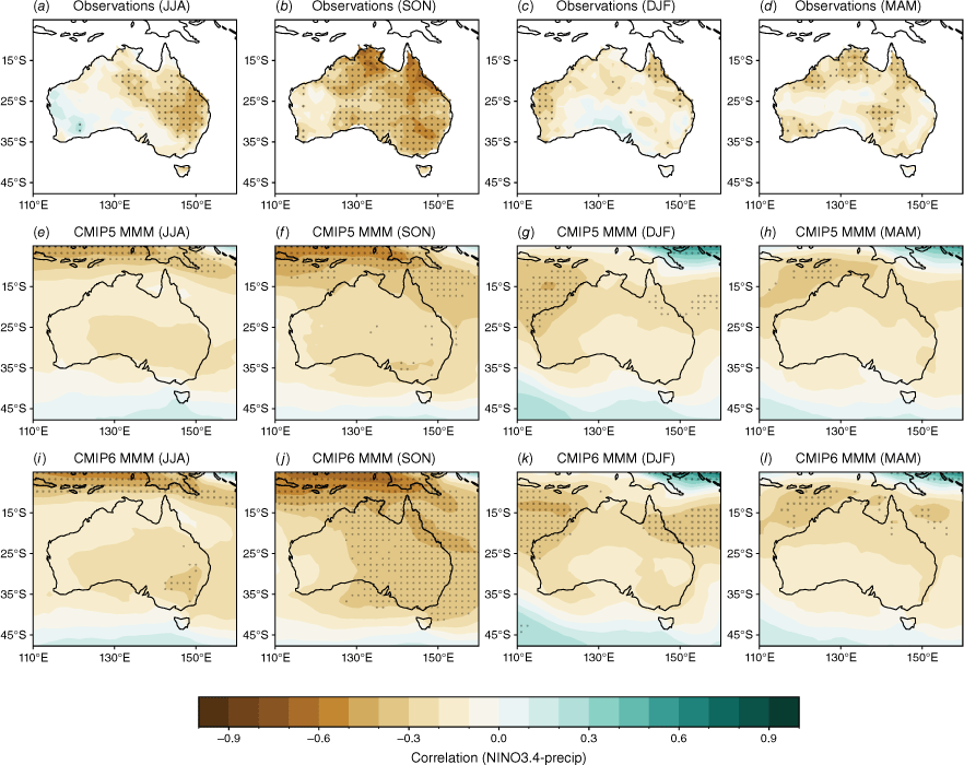
To evaluate the general teleconnections between ENSO and rainfall, we calculate the correlations between seasonal averages of rainfall and the concurrent Niño 3.4 index. The observed teleconnections (Fig. 2a–d) vary largely regionally and seasonally. They are strongest during SON, when correlations are significant over most of Australia except for Western Australia (WA). During JJA (Fig. 2a), the second-most teleconnected season, observed correlations are significant over parts of central and north-eastern Australia. During DJF and MAM (Fig. 2c–d), correlations are weaker and span parts of northern Australia and WA. The strong observed relationship during SON is reproduced in the CMIP5 and CMIP6 MMM, with a noticeable improvement in the SON teleconnection in CMIP6 (Fig. 2f, j). There is also a small improvement in the strength of the teleconnections in DJF, particularly over north-eastern Australia. However, models simulate the JJA teleconnections poorly.
Seasonal correlation between the Niño 3.4 index and precipitation in (a–d) AGCD observations, (e–h) CMIP5 and (i–l) CMIP6 models over 1950–2005. In the top row (observations), stippling indicates significance at the 90% confidence level according to a t-test. Stippling in the bottom two rows shows areas where 70% of models agree on the sign of the correlation and where 70% of models have a significant correlation at the 90% confidence level.
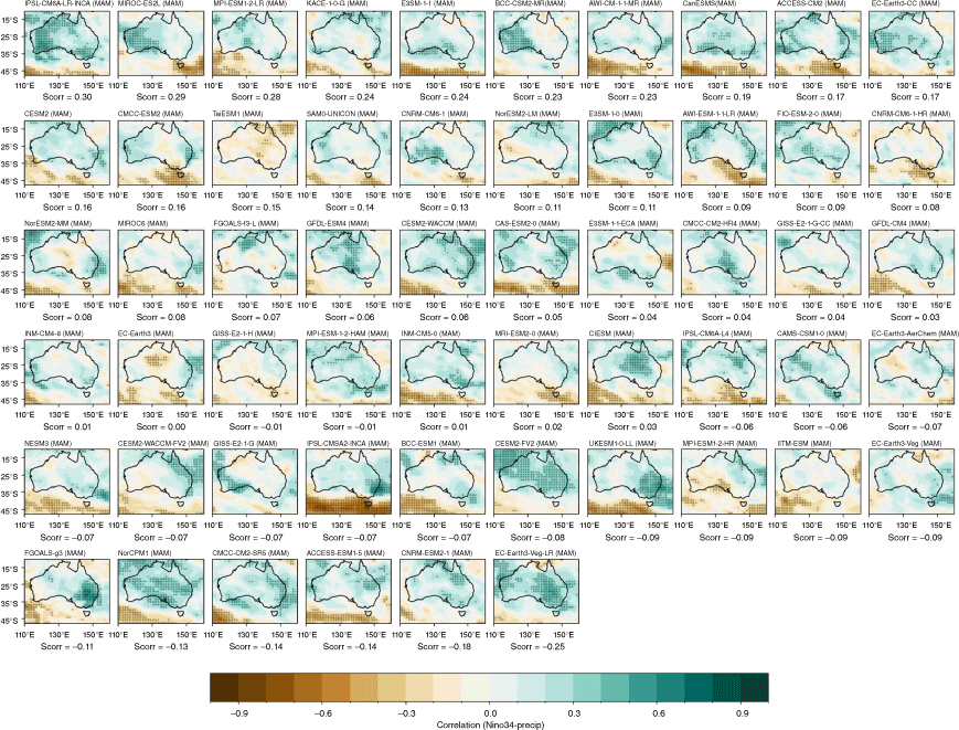
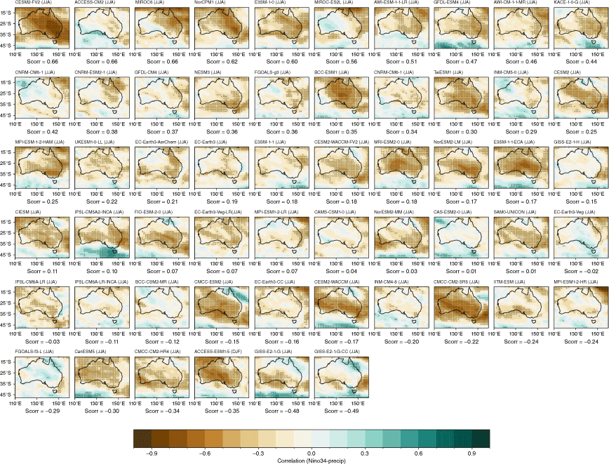
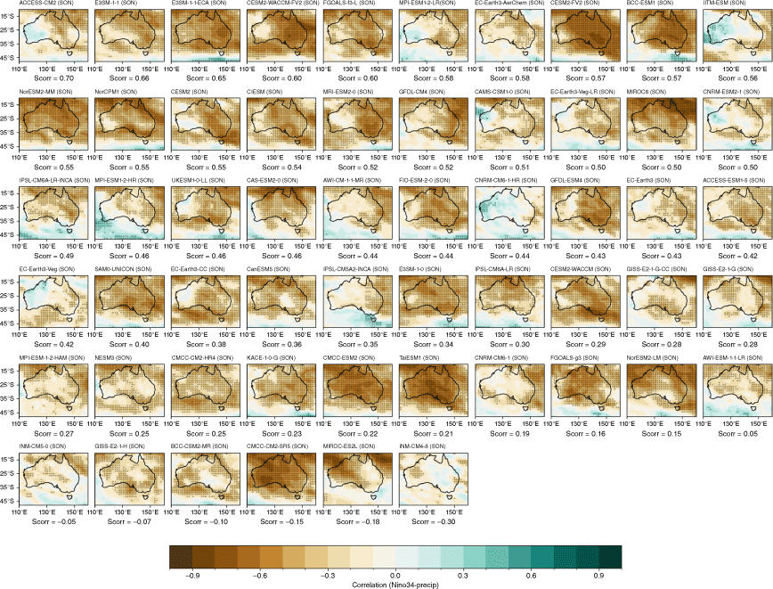
Recognising that the MMM does not capture the spread in each individual model performance, we also present the model and ensemble member spread for two metrics: spatial correlation of teleconnection patterns and correlation with all-Australian average rainfall. Fig. 3a shows the range of spatial correlation between each model’s simulated ENSO teleconnection pattern with the observed teleconnection pattern, not including the ocean points surrounding Australia. This is one measure of how well each model can simulate the observed spatial patterns shown in Fig. 2a–d. Repeating this analysis with root-mean-squared error (not shown) yields similar results. Perhaps not surprisingly, there is a large spread across CMIP models. The model spread in the correlation patterns is generally higher than the seasonal variations in the teleconnections (Fig. 3a), and is largest in JJA. This large spread could be due to model diversity in simulating the background climate, ENSO peak season, spatial patterns in SSTs and atmospheric teleconnections, or interaction between ENSO and other modes of variability such as the IOD (e.g. McKenna et al. 2020; Planton et al. 2021). Poor representation of ENSO life cycle in models (e.g. Taschetto et al. 2014, McKenna et al. 2020) could be one of many other reasons for the large spread. Due to these various potential complicating factors, a separate study is required to investigate the seasonality in model spread. However, CMIP6 models do exhibit improved mean spatial correlation and reduction in model spread during SON, and to a lesser extent during JJA. Maps of each individual model’s ENSO teleconnection patterns are shown in the Appendix (Fig. A1–A4), ranked by spatial correlation (highest to lowest) and also depict a large diversity in the representation of ENSO teleconnections.
(a) Spatial correlation between the observed Australian region ENSO patterns and those in the CMIP5 or CMIP6 models for each season, for each model’s first ensemble member. The boxes and whiskers indicate the spread of models, with the filled boxes showing where 50% of the models lie, and the whiskers showing the remaining upper and lower 25% of models. Circles indicate outliers. (b) Correlation between Nino3.4 and all-Australian rainfall for CMIP6 for individual ensemble members for SON only. Only models that have more than one ensemble member are shown here. Red indicates the first ensemble member (r1i1p1f1), which is commonly used to represent the model in many studies, including this one. Solid horizontal line indicates the observed correlation coefficient.
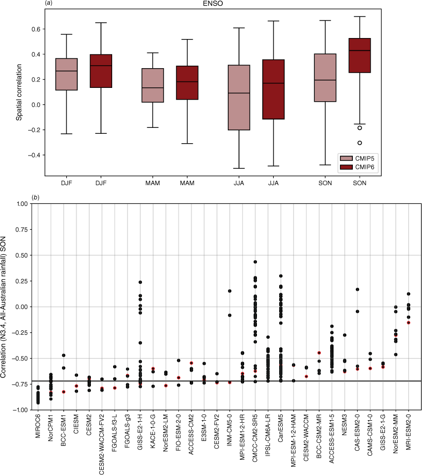
Additionally, 34 of the CMIP6 models have more than one ensemble member available, with a handful of ensembles with over 40 members (e.g. CANESM5 and MIROC6). As an indication of the internal variability within each model, Fig. 3b shows the correlation between Niño3.4 and all-Australian rainfall for SON. The first ensemble member (r1i1p1f1) – which is used as the representative run in many studies, including this one – is shown in red. For this metric, the ensemble spread is very large, particularly among the large ensembles, indicating high internal variability in the models. This corroborates previous studies that show that ENSO teleconnections can vary considerably between simulations performed with the same model, despite the same physics and parameterisations (e.g. see fig. 6 of Garcia-Villada et al. 2020). Additionally, in many models, for this particular metric, the first ensemble member is not necessarily the ‘best’ performing member (i.e. with the highest correlation). This is an important point to keep in mind in future evaluation or model selection studies, depending on the intended purpose and region of the evaluation. We note also that this is just one possible metric, another being the spatial correlation between observed and simulated teleconnection patterns (Supplementary Fig. S1).
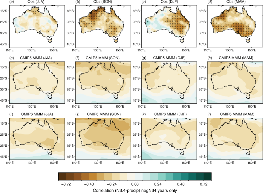
We now evaluate the models’ ability to reproduce the observed asymmetry of ENSO teleconnections by evaluating the relationship with Australian rainfall separately for positive Niño3.4 (representing El Niño) and negative Niño3.4 (representing La Niña) years. This asymmetry, in which La Niña years tend to have a more robust, and spatially different, correlation with Niño 3.4 compared to El Niño years, has been noted in previous studies (e.g. Cai et al. 2010, 2012; King et al. 2014; Chung and Power 2017). Positive and negative Niño3.4 years are identified using the DJF mean of the Niño3.4 index. Then, the concurrent correlation between ENSO phases and rainfall anomalies are shown in Fig. 4 for the negative values of Niño3.4 (negN34, i.e. Niño3.4 < 0) and in Fig. 5 for the positive Niño3.4 (posEN34, i.e. Niño3.4 > 0).
Seasonal correlation between the Niño3.4 index and precipitation in (a–d) AGCD observations over 1950–2005, (e–h) CMIP5 and (i–l) CMIP6 MMM for negative N34 years only. Stippling in the bottom two rows shows areas where 70% of models agree on the sign of the correlation and where 70% of models have a correlation significant at the 90% level; in observations, stippling indicates significance at the 90% confidence level according to a t-test.
Seasonal correlation between the Niño3.4 index and precipitation in (a–d) AGCD observations over 1950–2005, (e–h) CMIP5 and (i–l) CMIP6 MMM for positive N34 years only. Stippling in the bottom two rows shows areas where 70% of models agree on the sign of the correlation and where 70% of models have a correlation significant at the 90% level; in observations, stippling indicates significance at the 90% confidence level according to a t-test.
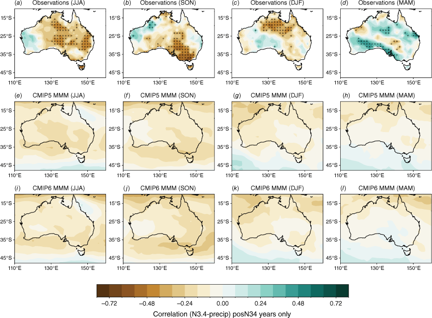
In this subsection we show that the pattern of seasonal teleconnections when considering posN34 and negN34 years separately (Fig. 4, 5) differs to the teleconnection patterns for all years (Fig. 2). For example, in observations during DJF, there is a significant teleconnection to rainfall over eastern Australia during negN34 years (Fig. 4c), but this shifts to northern Australia during posN34 years (Fig. 5c). Conversely, during JJA, there is a significant teleconnection to eastern Australian rainfall during posN34 years (Fig. 5a) but not negN34 years (Fig. 4a). During MAM and SON, north-western Australia exhibits a significant teleconnection during negN34 years (Fig. 4b, d) but not during posN34 years (Fig. 5b, d). Interestingly, during MAM, posN34 years exhibit a positive correlation in small regions of south-western and central Australia, indicating a tendency for rainfall increase during this season (Fig. 5d). One caveat to note is that there is a correlation between Niño3.4 and DMI, which makes it difficult to disentangle the asymmetry between ENSO years and IOD years. This is discussed further in Section 4. Another caveat is that the ENSO–Australian rainfall relationship oscillates on multi-decadal timescales (e.g. Power et al. 2006; Cai et al. 2010). This further complicates the teleconnections and is not fully captured in our relatively limited analysis period of 1950–2005. In Section 3.2.3, we highlight further the difference in the strengths of the teleconnections between CP and EP El Niño and La Niña events.
The stronger rainfall response during La Niña years is linked to the warmer western Pacific SSTs which occur during La Niña events, including a south-westward shift of the South Pacific Convergence Zone, enhancing convection over eastern Australia (Power et al. 2006; Cai et al. 2010; King et al. 2014). Precipitation is also enhanced over eastern Australia during La Niña events due to increased oceanic supply of moisture from the Tasman and Coral Seas (Holgate et al. 2022). A previous evaluation of CMIP5 models showed that the models tended to simulate these ENSO-related SST anomalies in the Pacific too close to Australia, and weak ENSO asymmetry, hence overestimating the impact of La Niña on Australian rainfall (Weller and Cai 2013). Fig. 4 and 5 show that, overall, the CMIP5 and CMIP6 MMMs do capture the El Niño–La Niña teleconnection asymmetry, exhibiting stronger teleconnections during negN34 years during September–May. One noticeable improvement in the CMIP6 MMM is a strengthening in the DJF and SON correlation over northern and north-east Australia for negN34 years (Fig. 4j, k). However, the large inter-model spread remains problematic and is a reason why the MMM panels in Fig. 4 and 5 lack any stippling. Model-by-model spatial correlations are presented in the Appendix (Fig. A5–A12).
In recent years, the important role that ENSO diversity plays on seasonal teleconnections to Australian rainfall has been highlighted (e.g. Freund et al. 2019; Santoso et al. 2019; Ma et al. 2022). Most previous studies focused on the impacts of El Niño diversity on Australian rainfall, with CP El Niños associated with more drying due to the proximity of the SST anomaly. We define CP and EP indices following Sullivan et al. (2016):
where and are the standardised Niño3 and Niño4 indices respectively. Correlating the CP index against rainfall for all years (Supplementary Fig. S2), the teleconnection pattern shifts dramatically from season to season. During SON, large correlation coefficients are seen over most of the country, barring parts of WA. During DJF the teleconnection is only significant over the Cape York Peninsula, whereas during MAM the teleconnection is significant over much of northern Australia. During JJA a significant teleconnection is observed over central-eastern Australia. In contrast, the EP index has a much weaker correlation to seasonal rainfall, with only parts of northern and eastern Australia showing significant correlation during SON, and small parts of WA and north-eastern Australia during DJF.
In the remainder of this section, we examine the impacts of CP and EP flavours during both El Niño and La Niña events separately. Instead of measuring this through correlation as in the previous sections, we present composites of seasonal rainfall during each type of event. Because of the relatively low sample size of CP and EP El Niño–La Niña years, composites allow us to compare the mean differences between each phase rather than the relationship with any particular index.
To select ENSO events, we first select events in which the DJF Niño3.4 index is larger than 0.5 times the DJF standard deviation. Note that we use each model’s individual standard deviation to define events, as each model’s variability differs. Then, for example, for El Niño years, a CP El Niño is defined to be when the DJF Niño4 index > DJF Niño3 index. An EP El Niño is defined to be when the DJF Niño3 index > DJF Niño4 index. For La Niña events, the opposite is true (e.g. CP La Niña when DJF Niño4 < DJF Niño3). This method of distinguishing CP and EP events using the relative strengths of Niño3 and Niño4 indices follows Sullivan et al. (2016), although we use a different method of selecting the ENSO events themselves. Once the event has been classified, the corresponding standardised seasonal rainfall anomalies for each type of event are composited. Note that this is a strict method of defining CP and EP events. If using a specific threshold, for example CP or EP index greater than 0.5 standard deviation, some recent events such as the 2015 El Niño would be classified as a mixed CP–EP event (e.g. Santoso et al. 2017). For the purposes of this study, however, we separate the two types.
Fig. 6 shows composites of seasonal rainfall anomalies for CP El Niño events (top three rows) and CP La Niña events (bottom three rows). The maps are stippled where a t-test indicates that the composites significantly differ from the mean seasonal anomalies at the 90% confidence level. The observations (Fig. 6a–d, m–p) show that over most of Australia in all seasons, CP La Niñas are wet and CP El Niños are dry. As expected, the most widespread significance is during SON mostly over northern and eastern Australia, with CP La Niña anomalies stronger than CP El Niño anomalies over those regions. During DJF, despite being generally wet (dry) during CP La Niña (El Niño), there is no significance on the maps aside from a small region in central Australia during CP El Niño. During MAM, the northern part of the Northern Territory shows significant wet (dry) anomalies during CP La Niña (El Niño). During JJA, central Australia shows significant dry anomalies during CP El Niño only.
Composites of standardised seasonal rainfall anomalies during CP El Niño (three top rows) and CP La Niña (three bottom rows) for AGCD observations over 1950–2005 (a–d, m–p) and the CMIP5 (e–h, q–t) and CMIP6 MMM (i–l, u–x). Stippling in the CMIP5 and CMIP6 maps shows areas where 70% of models agree on the sign of the correlation and where 70% of models have a correlation significant at the 90% level; in observations, stippling indicates significance at the 90% confidence level according to a t-test.
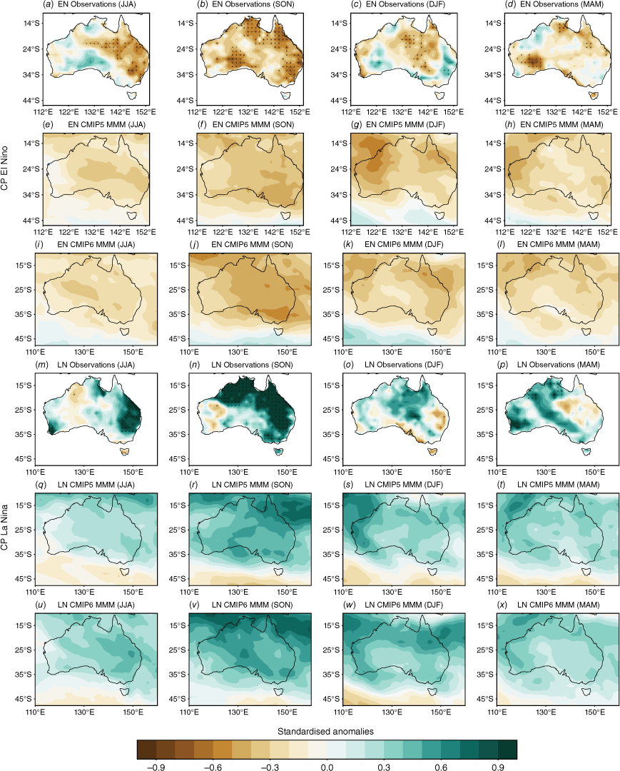
The models are able to capture the overall wet–dry La Niña–El Niño patterns; however, due to large inter-model spread, there is no stippling in any of the maps. It is worth noting that the CMIP6 MMM does show slightly stronger wet (dry) anomalies during CP La Niña (El Niño) years during SON, over northern and eastern Australia, indicating a modest improvement in the SON CP ENSO teleconnections.
In observations, EP La Niña ENSO events (Fig. 7a–d) overall have a much weaker correlation with Australian rainfall and, in contrast to CP La Niña ENSO events (Fig. 7m–p), observations exhibit a weaker Australian rainfall response, attributed to the unclear impact of EP La Niña. However, EP El Niño years are quite similar to CP El Niño years during JJA and SON. Significant dry anomalies appear to shift westward throughout the course of the year, starting over the north-east during JJA (Fig. 7a), moving over northern Australia during SON (Fig. 7b) and shifting to the north-west during DJF (Fig. 7c). There is no significant wet (dry) signal during MAM (Fig. 7d).
Composites of standardised seasonal rainfall anomalies during EP El Niño (three top rows) and EP La Niña (three bottom rows) for AGCD observations over 1950–2005 (a–d, m–p) and the CMIP5 (e–h, q–t) and CMIP6 MMM (i–l, u–x). Stippling in the CMIP5 and CMIP6 maps shows areas where 70% of models agree on the sign of the correlation and where 70% of models have a correlation significant at the 90% level; in observations, stippling indicates significance at the 90% confidence level according to a t-test.
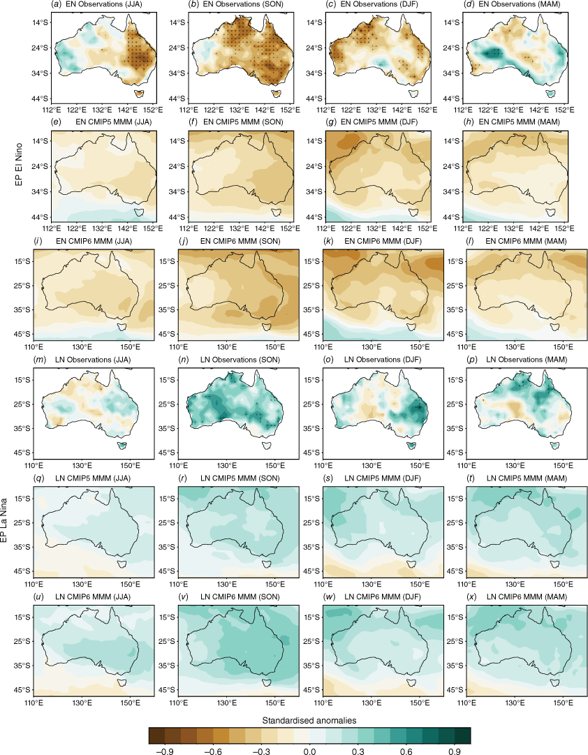
The models are able to replicate the weaker response to EP compared to CP La Niñas, particularly in JJA and SON (Fig. 6q–x and 7q–x). Although the CMIP6 MMM response to all El Niño and La Niña events has strengthened slightly in SON compared to CMIP5, the large inter-model spread again means that less than 70% of models agree on both the sign and significance of the correlation.
From this section we conclude that models can capture the overall stronger response to negN34 years and compared to posN34 years, and CMIP6 shows some improvement in the strength of the teleconnections during SON. They can also distinguish between the responses to CP and EP La Niña events, capturing the weaker rainfall responses during EP La Niña events in winter–spring (JJASON). We note also that, for consistency, in this study we used DJF CP and EP indices to define events, which may be an issue for those models that have inaccurate ENSO phase-locking.
4IOD and its impact on Australian climate
In this section, we present a literature review of studies that have evaluated CMIP6 models’ skill in simulating IOD variability (Section 4.1). In Section 4.2 we evaluate the simulated teleconnections between IOD and seasonal Australian rainfall, including the asymmetry in this relationship and implications of the co-variance between ENSO and the IOD. As the IOD is only active during austral winter and spring, we present results for JJA and SON only.
4.1 Evaluation of IOD variability
There have been mixed results in the simulation of IOD variability from CMIP5 to CMIP6. Among the improvements are a better overall simulation of the 3–5-year IOD cycle, and a well-captured seasonality of the IOD, with a peak in SON (McKenna et al. 2020). However, the IOD tends to peak 1 month earlier than observed in CMIP6 (September instead of October), likely affecting teleconnections to Australia. In CMIP5, most models simulated a peak in November (McKenna et al. 2020). Although the seasonality of the IOD remains overall well captured, the overly strong IOD bias that has persisted throughout generation of climate models (e.g. Cai and Cowan 2013) continues to exist in CMIP6. Furthermore, the pIOD skewness that was correctly captured in CMIP5, has been reduced significantly in CMIP6, with many CMIP6 models showing negative skewness (McKenna et al. 2020).
There are still underlying biases that compromise a realistic simulation of Indian Ocean processes and teleconnections to Australian climate (Jourdain et al. 2013; Grose et al. 2020; McKenna et al. 2020). For example, CMIP5 and CMIP6 models tend to overestimate the IOD amplitude. Underlying this bias is a too-strong thermocline–SST feedback in the equatorial Indian Ocean associated with an unrealistic upward tilting of the climatological thermocline toward the eastern Indian Ocean (Cai and Cowan 2013). The thermocline bias persists and slightly worsens in CMIP6 models (Wang et al. 2021) linked to greater bias in the strength of the equatorial easterly winds. These biases can affect the reliability of projections of IOD amplitude and frequency (Wang et al. 2017b, 2021) and are expected to affect teleconnections to Australian climate with an interplay with biases in the Pacific (Weller and Cai 2013; Grose et al. 2020).
Additionally, nearly half of CMIP6 models also do not accurately simulate the observed asymmetry of the IOD, i.e. that pIOD events tend to be stronger than nIOD events, an aspect that has degraded in CMIP6 compared to CMIP5 (Jourdain et al. 2013; McKenna et al. 2020). Although CMIP6 models demonstrated a notable improvement in the simulation of the tropical Pacific mean-state that led to some improvements in the simulation of ENSO variability, it appears that further efforts are required to resolve biases in the Indian Ocean.
4.2 Evaluation of IOD teleconnections to Australian climate
Although IOD variability is overestimated in most CMIP models, they underestimate the IOD teleconnections to Australian rainfall. Di Virgilio et al. (2022) noted a large spread in the ability of CMIP6 models to simulate this teleconnection and found that some models that simulated the ENSO–rainfall teleconnection well, performed poorly in simulating the IOD–rainfall relationship. Nevertheless, some CMIP6 models exhibit improved teleconnection over southern Australia and WA, but these models do not necessarily simulate the ENSO teleconnections well (Grose et al. 2020; Di Virgilio et al. 2022).
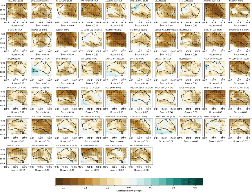
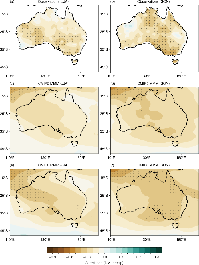
We measure the teleconnections between the IOD and Australian rainfall through the correlation between seasonal means of the DMI and rainfall. These correlations are strongest during SON in both observations and models (Fig. 8b, d, f). Compared to CMIP5, the CMIP6 MMM exhibits improved overall strength of the teleconnections, with stronger agreement across CMIP6 models than CMIP5 over WA in JJA and in many regions over Australia in SON.
Seasonal correlation between the DMI index and precipitation in (a–b) AGCD observations over 1950–2005, (c–d) CMIP5 and (e–f) CMIP6 models (bottom two rows). Stippling in the bottom two rows shows areas where 70% of models agree on the sign of the correlation and where 70% of models have a significant correlation at the 90% level. In the top row (observations), stippling indicates significance at the 90% confidence level according to a t-test.
There is also an asymmetry in the observed teleconnections between pIOD and nIOD years. The pIOD years tend to affect larger regions of Australia compared to nIOD years, particularly during JJA where much of north-western and central Australian rainfall is significantly correlated with the DMI (Fig. 9a–d; Cai et al. 2010, 2012). Representing this asymmetry in models is complex as the physical mechanisms underlying the teleconnections between the Pacific and Indian Ocean differ for El Niño–La Niña and pIOD–nIOD years (Cai et al. 2010, 2012). A previous study showed that CMIP5 models managed to simulate the IOD asymmetry; however, the models’ performance was distorted by biases in the representation of ENSO (Weller and Cai 2013). However, as ENSO and the IOD are known to co-vary, disentangling the impacts of the two is not straightforward (e.g. Ashok et al. 2003; Meyers et al. 2007; Liguori et al. 2022). In order to measure the independent component of the IOD, previous studies have used statistical methods such as partial regression analysis (e.g. Risbey et al. 2009; Cai et al. 2011) or an empirical orthogonal function-based IOD index, which does not correlate with ENSO (Meyers et al. 2007). Recently, Liguori et al. (2022) conducted pacemaker-type experiments to isolate the influence of ENSO and IOD on Australian rainfall by suppressing ENSO variability and decoupling the Indian Ocean separately. They compared the results of these experiments using statistical methods, finding that statistically removing the DMI from the Niño3.4 index led to ENSO teleconnections being underestimated. This is to be expected because strong ENSO events tend to induce IODs, so by subsampling non-IOD years, only weak ENSO events are left.
JJA and SON seasonal correlation between the positive IOD (pIOD, left two columns) and negative IOD (nIOD, right two columns) indices and precipitation in (a–d) AGCD observations over 1950–2005, (e–h) CMIP5 and (i–l) CMIP6 MMM. Stippling in the bottom two rows shows areas where 70% of models agree on the sign of the correlation and where 70% of models have a correlation significant at the 90% level; in observations, stippling indicates significance at the 90% confidence level according to a t-test.
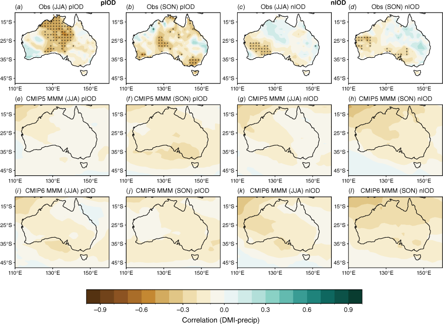
However, they also found that in physically removing the IOD or ENSO, their model experiments were subject to the biases described above, namely the overestimation of IOD variability, and that results differed when applied to observed or modelled output. In the same study, the authors present a statistical model to describe June–October rainfall, which consists of a linear combination of the Niño3.4 and DMI indices. Although the statistical model of Liguori et al. (2022) presents a useful framework, it also highlights the complexities of disentangling the co-variance of ENSO and the IOD. Fig. 9 shows the JJA and SON correlation between DMI and rainfall for pIOD and nIOD years separately, using the SON DMI to distinguish between pIOD and nIOD years. In observations, pIOD years show a significant correlation between DMI and rainfall across most of central Australia during JJA, and southern Australia during SON. The nIOD shows significant correlation over parts of WA during JJA and SON, and small parts of southern Australia during SON. The CMIP5 and CMIP6 MMMs both show that the models generally perform fairly poorly in simulating the IOD asymmetry. In fact, over our analysis period (1950–2005), many nIOD years coincide with La Niña years, and vice versa, so the models show a somewhat stronger correlation between rainfall and DMI during negative IOD years, contrary to observations. Previous CMIP5 results (Weller and Cai 2013) showed an underestimation of IOD asymmetry due to the westward extension of La Niña (i.e. boosting the nIOD impact). In CMIP6, this may be lessened due to the reduction in cold tongue bias. However, this may also be negated by the reduction in IOD skewness in CMIP6 (McKenna et al. 2020), leading to no apparent improvement in CMIP6 in terms of IOD asymmetry teleconnection.
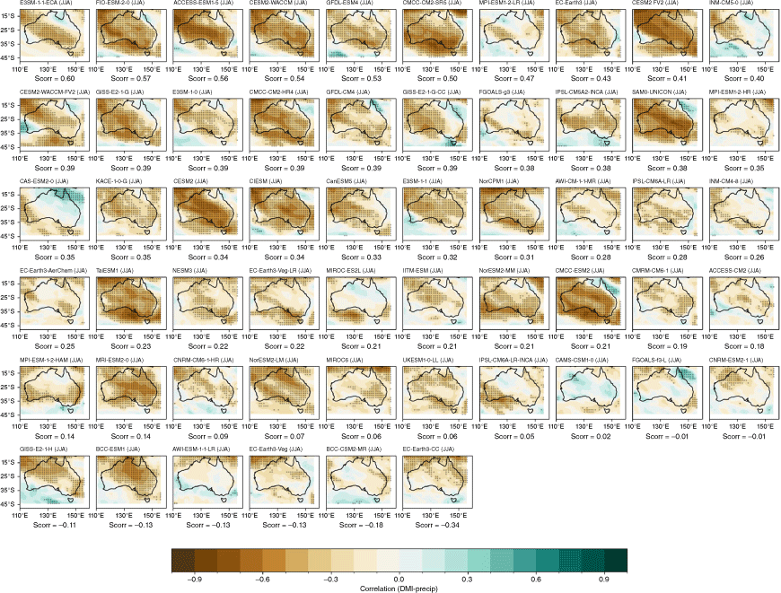
There is an extremely large spread in the individual model performances, and among ensemble members within the same model, as shown by the seasonal spatial correlation between modelled and observed teleconnection patterns (Fig. 10). During JJA, some CMIP6 models exhibit a marginal improvement in the spatial representation of teleconnection patterns; however, there is no improvement during SON. The inter-model spread is also wider in CMIP6 than in CMIP5 (Fig. 10a). As with ENSO, Fig. 10b shows an extremely large spread among individual ensemble members in the range of correlation between SON DMI and all-Australian rainfall. Again, using this metric, the first ensemble member (‘r1i1p1f1’) is often not the highest performing. An alternative metric, spatial correlation between observed and modelled SON patterns for each ensemble member, is shown in Supplementary Fig. S3. As an illustration of how the use of different metrics to measure skill might affect a model or ensemble member’s ranking differently, consider BCC-CSM2-MR’s r1i1p1 member. This member simulates the highest DMI–rainfall correlation among the three members available (Fig. 10b), and also yields the lowest spatial correlation pattern of the three members (Supplementary Fig. S3). The maps of each individual models’ teleconnection patterns are shown in the Appendix, Fig. A13 and A14, ranked by spatial correlation.
(a) Spatial correlation between the observed Australian region IOD teleconnection patterns and those in the CMIP5 or CMIP6 models for each season; the closer to 1, the more accurate the representation of the teleconnection patterns. The boxes and whiskers indicate the spread of models, with the filled boxes showing where 50% of the models lie, and the whiskers showing the remaining upper and lower 25% of models. Circles indicate outliers. (b) Correlation between DMI and all-Australian rainfall for individual CMIP6 ensemble members for SON only. Only models with more than one ensemble member are shown here. Red indicates the first ensemble member (r1i1p1f1), which is commonly used to represent the model in many studies, including this one. Solid horizontal line indicates the observed correlation coefficient.
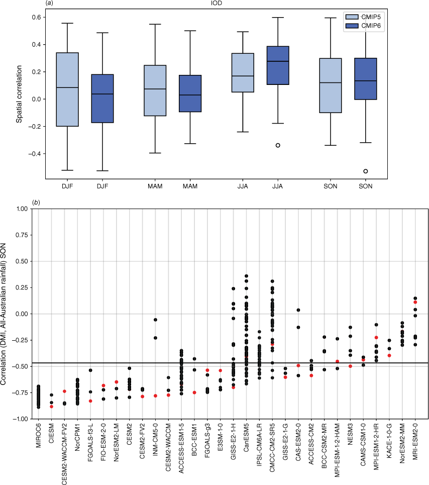
In comparing the inter-model spread in spatial correlation for ENSO and IOD teleconnections (Fig. 3a, 10a), we find that the two metrics are largely similar. However, one interesting finding is that the inter-model spread for JJA IOD teleconnections is much more constrained than for ENSO teleconnections. This is possibly because the IOD teleconnection pattern in JJA is more spatially uniform over Australia, whereas the ENSO teleconnection pattern has a dipole structure that is more difficult for models to reproduce.
5SAM and its impact on Australian climate
In this section, we discuss the ability of CMIP6 models to simulate SAM variability and biases in the mid-latitude westerly winds (Section 5.1). In Section 5.2 we evaluate the skill of the CMIP models in simulating the SAM teleconnections to seasonal Australian rainfall.
5.1 Evaluation of SAM metrics in CMIP6
Zhang et al. (2021) evaluated CMIP6 models in their ability to capture the SAM spatial pattern and found that the basic features are well reproduced in the MMM, with the highest skill in summer (DJF) and lowest skill in autumn (MAM). They found that, in general, models slightly overestimate the SAM amplitude in most seasons except in MAM. They linked this bias to a poor simulation of the spatial asymmetric part of SAM. Indeed, whereas the SAM is predominantly zonally symmetric, some zonal asymmetries do exist in its structure, particularly outside of summer (Boschat et al. 2023).
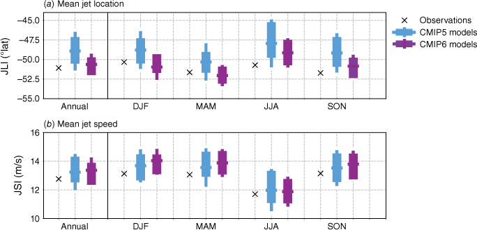
As SAM is intrinsically related to the variations in the eddy-driven jet, we examine biases in the location and the speed of the mid-latitude westerly winds or jet. This is a mid-latitude wind belt that encircles the globe, flowing from west to east and is associated with storm tracks that bring rainfall. It persists year-round and is typically measured in terms of its strength and latitude. Although the latitudinal shift of the winds is associated with the phase of SAM, its strengthening or weakening does not necessarily co-occur with changes in its latitude. It can therefore be useful to diagnose these jet diagnostics individually (Baker et al. 2017; Bracegirdle et al. 2020). Fig. 11 shows that the simulation of the mean 850-hPa jet location and speed has improved somewhat in CMIP6 models. The CMIP5 models tend to simulate a jet that was too far equatorward, and this bias has reduced in CMIP6, along with a slightly smaller spread in the CMIP6 ensemble (Goyal et al. 2021). The variability in these metrics is also remarkably well simulated (not shown), in line with Bracegirdle et al. (2020) who find an improvement in CMIP6 jet variability that they quantify through a reduced bias in the decorrelation timescale of the SAM (i.e. a less persistent SAM).
Annual and seasonal mean (a) position and (b) speed of the westerly polar jet during 1979–2005 in ERA5 reanalyses, CMIP5 and CMIP6 models. Jet speed is defined every month as the maximum of zonal mean 850-hPa zonal winds between 10 and 75°S, and jet position indicates the latitude of this maximum.
5.2 Evaluations of SAM teleconnections to Australian climate
The impact of SAM on Australia’s climate is closely linked to the seasonal movement and strength of the westerly jet. In summer and spring, the poleward shift of the jet associated with positive SAM allows easterlies to bring moist onshore flow to eastern Australia. In winter, when the jet is climatologically closer to the equator (compared to summer), a poleward shift leads to drier conditions over southern Australia (Hendon et al. 2007).
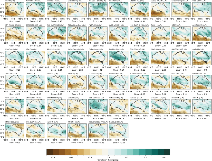
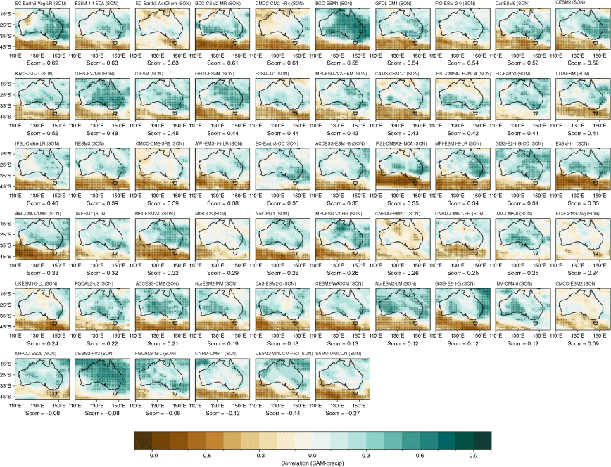
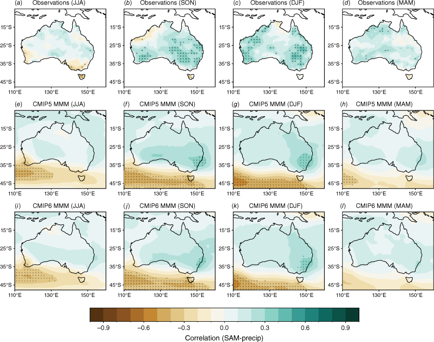
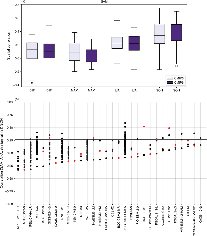
The CMIP5 and CMIP6 models are able to capture the main features and seasonality of the SAM influence on Australian rainfall, with positive SAM associated with wetter conditions across eastern Australia particularly in SONDJF (Fig. 12b, c), and more pronounced drying in southwest WA, Tasmania and Victoria in JJA (Fig. 12a). However, the MMM correlation patterns are slightly weaker for CMIP6 compared to CMIP5, due to a larger intermodel spread, particularly in JJA and SON (Fig. 13a). The spread in the correlation between the SON SAM index and all-Australian averaged rainfall among ensemble members is also extremely large (Fig. 13b). Spatial correlations of the observed and modelled SON teleconnections are shown in Supplementary Fig. S4. Maps of individual models’ teleconnections, sorted by spatial correlation, are shown in the Appendix (Fig. A15–A18). A few outlier CMIP6 models fail to capture any part of the relationship.
Seasonal correlation between the SAM index (based on Marshall 2003) and precipitation in (a–d) AGCD observations over 1950–2005, (e–h) CMIP5 and (i–l) CMIP6 MMM. Stippling in the bottom two rows shows areas where 70% of models agree on the sign of the correlation; in observations, stippling indicates significance at the 90% confidence level according to a t-test.
(a) Spatial correlation between the observed SAM teleconnection patterns and those in the CMIP5 or CMIP6 models for each season; the closer to 1, the more accurate the representation of the teleconnection patterns. The boxes and whiskers indicate the spread of models, with the filled boxes showing where 50% of the models lie, and the whiskers showing the remaining upper and lower 25% of models. Circles indicate outliers. (b) Correlation between SAM index and all-Australian rainfall for individual CMIP6 ensemble members for SON only. Only models which have more than one ensemble member are shown here. Red indicates the first ensemble member (r1i1p1f1), which is commonly used to represent the model in many studies, including this one. Solid horizontal line indicates the observed correlation coefficient.
The SAM and zonal mean jet diagnostics used here are relevant to examine hemispheric-scale climate impacts; however, we need to bear in mind that the SAM as well as the jet contain important spatial asymmetries (particularly in seasons outside of summer). Evaluating the ability of climate models to simulate more sectoral jets and smaller-scale processes that affect regional teleconnections will be of particular relevance to current and future climate impacts in Australia.
6Long-term trends
We now briefly discuss the observed and simulated trends in ENSO, IOD and SAM over the historical period. As the ENSO and IOD indices used here are derived from SSTs, the predominant long-term trend for 1950–2005 is the anthropogenic warming trend. This warming trend, particularly in the western Pacific, has been accompanied by an observed shift towards more frequent CP El Niño events as compared to EP El Niño events (e.g. Freund et al. 2019; Wang et al. 2019). To measure any trend in the overall amplitude of year-to-year variability in the amplitude of ENSO and the IOD, we calculate the trend in the seasonal standard deviation of a 10-year running window of the Niño3.4 index and DMI. In observations and models, there is no significant trend in the amplitude of ENSO or IOD variability in any season (not shown). We note, however, that 10 years is a relatively short window, considering that Pacific and Indian Ocean SSTs experience significant decadal variability. Using coral reconstructions over the past 400 years, Freund et al. (2019) show an increasing trend in the frequency of CP relative to EP El Niño. Also using reconstructions, Abram et al. (2020) show an increase in the frequency and strength of pIOD over the last millennium, with extreme pIOD events (such as the 1997 event) being rare before 1960. Recent studies using longer analysis periods have found that, under a high emissions future, ENSO-related SST variability is projected to display a relatively small increase in CMIP6 under all scenarios (Cai et al. 2022).
On decadal timescales, the Interdecadal Pacific Oscillation (IPO; Power et al. 1999) also strongly modulates ENSO’s impacts on Australian climate. During positive IPO phases, the background state of the Pacific is more El Niño-like, and ENSO teleconnections to Australian rainfall are weakened. During negative IPO phases, the opposite happens (Power et al. 1999; Salinger et al. 2001; Heidemann et al. 2022). Although a detailed assessment of the IPO and associated impacts in CMIP models is outside the scope of this study, several previous studies have noted an underestimation of decadal variability in previous generations of climate models (e.g. Henley et al. 2015; Kociuba and Power 2015), linked to the common biennial ENSO bias. An improvement in the simulation of interdecadal global mean temperature variability has been noted in CMIP6 (Parsons et al. 2020), though this may not be related to the improvements in the tropical Pacific.
The Indian Ocean also undergoes decadal variability in an IOD-like pattern (e.g. Kripalani and Kumar 2004), which in turn modulates the IOD intensity. Previous studies have linked this decadal variability to feedbacks linked to the Walker circulation, and is driven by the IPO (e.g. Huang et al. 2019). The CMIP6 models can reproduce decadal variability in the tropical Indian Ocean to some extent, though many models underestimate its amplitude (Halder et al. 2021). The Indian Ocean SST has also experienced a long-term trend, with the western side warming at a faster rate than any other tropical ocean regions (Roxy et al. 2014). This non-uniform IOD-like warming has been attributed to the increase in anthropogenic greenhouse gases (Du and Xie 2008), ENSO asymmetry (Roxy et al. 2014) and increased heat transport from the tropical Pacific in recent decades (Dong and McPhaden 2017). Numerical experiments suggest that the long-term warming of the Indian Ocean can accelerate the Pacific Walker Circulation and reduce precipitation in the tropical Atlantic (Dhame et al. 2020). However, the non-uniform warming of the Indian Ocean is not captured by CMIP models.
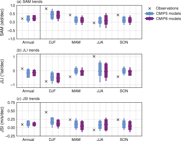
In recent decades, the SAM has experienced a poleward shift and intensification of the jet that has been observed in DJF at least partly due to ozone depletion (Masson-Delmotte et al. 2021; Morgenstern 2021). However, trends in other seasons are too weak or uncertain as models fail to simulate the seasonality of observed trends outside of summer. Models successfully capture the DJF poleward shift and we find a slight improvement in the CMIP6 simulation of annual mean SAM and jet trends, although Fig. 14 shows that this may stem from compensating errors in different seasons. The SAM trends are generally underestimated in both CMIP5 and CMIP6 models, particularly in MAM and SON, when the SAM is known to be more asymmetric. Trends in the 850-hPa jet location and speed are also largely underestimated in JJA and DJF respectively, potentially due to model deficiency in capturing the effect of sea-ice change on jet-location shift (e.g. Screen et al. 2022), response to atmospheric chemistry (e.g. Morgenstern 2021) and mean-state biases (e.g. Kajtar et al. 2021). Additionally, the latitudinal mean position of the southern hemisphere eddy-driven jet is biased equatorward in all CMIP3 models (Kidston and Gerber 2010) and many CMIP5 models (Barnes and Polvani 2013). Given that the mean latitude of the jet affects the variability of the annual modes (Kidston and Gerber 2010), an incorrect representation of the eddy-driven jet can influence biases in the SAM, which in turn affects the weather systems and associated precipitation over the southern and eastern parts of Australia.
Annual and seasonal mean trends in (a) SAM, (b) position and (c) speed of the westerly jet over 1979–2005 in ERA5 reanalyses, CMIP5 and CMIP6 models. Jet speed is defined every month as the maximum of zonal mean 850-hPa zonal winds between 10 and 75°S, and jet position indicates the latitude of this maximum.
7Discussion and conclusions
The representation of regional climate drivers and their interactions with Australian climate is an important aspect of climate models that should be carefully considered before drawing model-based conclusions on regional climate variability and change. In this study, we evaluated major nodes of variability that influence Australia’s climate, in CMIP5 and CMIP6 models. Our evaluations have shown that CMIP6 data have a significant improvement to springtime teleconnections between ENSO and Australian rainfall. Both CMIP5 and CMIP6 models are generally able to capture the asymmetry in the impacts of El Niño and La Niña events, as well as the differing responses between CP and EP La Niña events, with some improvement in the spring and summertime teleconnections to northern and north-east Australia during La Niña years. However, a large inter-model spread in the simulation of these teleconnections remain, and the simulation of autumn- and winter-time teleconnections have not improved.
The simulation of IOD teleconnections is more varied. Although the overall strength of winter- and spring-time teleconnections has improved in CMIP6, the spatial representation of these teleconnections has not. The inter-model spread in IOD teleconnections in CMIP6 is larger than in CMIP5, increasing the uncertainty in future projections.
Although the representation of SAM variability has improved considerably in most seasons, teleconnections between SAM and Australian rainfall appear to have degraded from CMIP5 to CMIP6 due to substantially larger inter-model spread, particularly in winter and spring.
In recent years, it has become especially apparent that compound events arising from the interactions among ENSO, IOD and SAM can have major impacts on rainfall, temperature and other climate variables. When two or more climate drivers operate concurrently, the consequences can be severe and can result in extreme heat and drought, or very wet seasons. This study is a step towards evaluating the models’ ability to simulate these climate events, but a full evaluation of these interactions between climate drivers in CMIP6 is needed to provide a more comprehensive understanding of the models’ skill.
Another major question is how these drivers and teleconnections will change in the future. Recent work has found that approximately half of the regions that have temperatures and precipitation affected by ENSO in DJF are projected to experience an amplification of these impacts under a high-emissions future (Power and Delage 2018; Yeh et al. 2018; McGregor et al. 2022).
One additional issue to note is the large spread in the performance of ensemble members, particularly in the models with large ensembles, indicating high internal variability. Although we only assess the ensemble spread in one metric in Fig. 3, 10 and 13 (teleconnection with all-Australian rainfall), performance in other metrics may differ. However, one important point to note for future model evaluation and selection efforts is that the first ensemble member, commonly used as representative of a model’s performance, is not necessarily the ‘best’ performing member, depending on the particular metric or region it is being evaluated against. As this study is intended to present a general evaluation across all seasons and regions, we do use the first member; however, it may be more appropriate in future downscaling or evaluation studies to choose differently, or to use all available ensemble members. A recent study found that >50 ensemble members are needed to capture baseline characteristics of ENSO and >6 members are needed to capture remote ENSO teleconnections globally (Lee et al. 2021). However, given the large inter-model spread shown in this study, it is apparent that ENSO teleconnections to the Australian region are much less constrained than ENSO teleconnections to other tropical ocean basins, for example.
What do our results mean for projections of future climate? In summary, the improvements in CMIP6 shown in this report offer a small degree of increased confidence in springtime projections of ENSO- and IOD-related rainfall change in most regions, excluding WA. We also highlight the differences in regional rainfall responses between EP and CP El Niño and La Niña years. Though some of these differences are captured by models, there is much room for improvement. As is the nature of understanding and modelling such complicated processes, there have been no giant leaps in model performance.
In Table 1, we list the five models which have the highest spatial correlation between modelled and observed teleconnections, for each driver and each season, for the first ensemble member. Although there are some limitations to this selection criterion, it provides an indication of how well the teleconnections are simulated. To compare this to other studies, the models that are part of the seven selected for optimal downscaling by Grose et al. (2023) are shown in bold, whereas models that are in the same family are shown in italic. Although Grose et al. (2023) did not base their selection purely on model performance, it is interesting to note that many of the selected models (or family of models) also simulate teleconnections particularly well in SON, and less so in JJA. Other models which perform ‘well’ according to this metric include models from the CESM2, EC-Earth3 and ACCESS families.
| DJF | MAM | JJA | SON | ||
|---|---|---|---|---|---|
| ENSO (all years) | TaiESM1 | GFDL-CM4 | CESM2-FV2 | ACCESS-CM2 | |
| EC-Earth3-AerChem | MIROC6 | ACCESS-CM2 | E3SM1-1 | ||
| CAM5-CSM1-0 | GISS-E2-1-H | MIROC6 | E3SM1-1-ECA | ||
| IPSL-CM6A-LR-INCA | IPSL-CM6A-LR | NorCPM1 | CESM2-WACCM-FV2 | ||
| CESM2-WACCM-FV2 | NorESM2-MM | E3SM-1-0 | FGOALS-f3-L | ||
| La Niña years | CNRM-ESM2-1 | MCM-UA-1-0 | UKESM1-0-LL | IPSL-CM6A-LR-INCA | |
| E3SM-1-1 | GISS-E2-1-G-CC | TaiESM1 | MRI-ESM2-0 | ||
| CAMS-CMS1-0 | CAS-ESM2-0 | EC-Earth3 | E3SM-1-0 | ||
| TaiESM1 | IPSL-CM6A-LR | IPSL-CM6A-LR | TaiESM1 | ||
| CMCC-CM2-SR5 | GISS-E2-1-G | AWI-CM-1-1-MR | IPSL-CM6A-LR | ||
| El Niño years | CESM2-WACCM-FV2 | FGOALS-f3-L | BCC-ESM1 | BCC-ESM1 | |
| EC-Earth3-Veg-LR | EC-Earth3-AerChem | AWI-ESM-1-1-LR | EC-Earth3-CC | ||
| CESM2 | NESM3 | INM-CM5-0 | TaiESM1 | ||
| CESM2-WACCM | TaiESM1 | CESM2 | EC-Earth3-Veg | ||
| AWI-CM-1-1-MR | CESM2-WACCM-FV2 | ACCESS-CM2 | EC-Earth3-Veg-LR | ||
| IOD | E3SM-1-1-ECA | FGOALS-f3-L | |||
| FIO-ESM-2-0 | EC-Earth3-CC | ||||
| ACCESS-ESM1.5 | GFDL-ESM4 | ||||
| CESM2-WACCM | SAM0-UNICON | ||||
| GFDL-ESM4 | ACCESS-CM2 | ||||
| SAM | CESM2-FV2 | IPSL-CM6-LR-INCA | NESM3 | EC-Earth3-Veg-LR | |
| CIESM | MIROC-ES2L | AWI-CM-1-1-MR | E3SM-1-1-ECA | ||
| AWI-CM-1-1-MR | MPI-ESM1-2-HR | GISS-E2-1-H | EC-Earth3-AerChem | ||
| MPI-ESM1-2-LR | KACE-1-0-G | EC-Earth3-Veg | BCC-CSM2-MR | ||
| MIROC-ES2L | E3SM-1-1 | MPI-ESM2-1-2-HAM | CMCC-CM2-HR4 |
Models in bold were also selected as the downscaling choices in Grose et al. (2023), and models in italic are in the same family as the models in bold.
Although global efforts in climate modelling have yielded stark improvements over the years, there are clearly many areas in which models still fall short. At the same time, the world continues to warm at an unprecedented rate, causing changes to the climate system which manifest in more frequent and severe extreme events. To provide the best possible information to improve preparedness for these impacts, it is crucial that the scientific community continues to better understand how climate drivers and interactions will change, and climate models remain the best tool available to us to do so.
Data availability
The CMIP6 model output that was analysed in this study is publicly available from https://esgf.nci.org.au/projects/esgf-nci/. Observed monthly means of rainfall totals from the Australian Gridded Climate Dataset are publicly available at https://doi.org/10.4227/166/5a8647d1c23e0. Observed SSTs used to calculate Nino3.4 and DMI indices are available at https://psl.noaa.gov/data/gridded/data.noaa.ersst.v5.html. ERA-5 reanalysis output used to compute jet speed and location is available at https://cds.climate.copernicus.eu/cdsapp#!/dataset/reanalysis-era5-complete. Observed Marshall SAM indices are available at https://legacy.bas.ac.uk/met/gjma/sam.html. Code is available upon request from C. Chung.
Declaration of funding
This work was supported with funding from the Australian Government’s National Environmental Science Program. This work has also been supported by the Victorian Department of Energy, Environment, and Climate Action under the Victorian Water and Climate Initiative. This research was undertaken with the assistance of resources and services from the National Computational Infrastructure (NCI), which is supported by the Australian Government.
Conflicts of interest
Andréa Taschetto is an Associate Editor of the Journal of Southern Hemisphere Earth Systems Science (JSHESS) but did not at any stage have editor-level access to this manuscript while in peer review, as is the standard practice when handling manuscripts submitted by an editor to this journal. JSHESS encourages its editors to publish in the journal and they are kept totally separate from the decision-making processes for their manuscripts. The authors have no further conflicts of interest to declare.
Acknowledgements
The authors thank the anonymous reviewers, Roseanna McKay, Andrew Dowdy, Pandora Hope, David Jones, Chun Hsu Su and Chris Lucas for helpful feedback.
References
Abram NJ, Wright NM, Ellis B, et al. (2020) Coupling of Indo-Pacific climate variability over the last millennium. Nature 579, 385-392.
| Crossref | Google Scholar |
Ashok K, Guan Z, Yamagata T (2003) Influence of the Indian Ocean Dipole on the Australian winter rainfall. Geophysical Research Letters 30(15), 1821.
| Crossref | Google Scholar |
Baker HS, Woollings T, Mbengue C (2017) Eddy‐driven jet sensitivity to diabatic heating in an idealized GCM. Journal of Climate 30(16), 6413-6431.
| Crossref | Google Scholar |
Barnes EA, Polvani L (2013) Response of the midlatitude jets, and of their variability, to increased greenhouse gases in the CMIP5 models. Journal of Climate 26, 7117-7135.
| Crossref | Google Scholar |
Boschat G, Purich A, Rudeva I, Arblaster J (2023) Impact of zonal and meridional atmospheric flow on surface climate and extremes in the Southern Hemisphere. Journal of Climate 36, 5041-5061.
| Crossref | Google Scholar |
Bracegirdle TJ, Holmes CR, Hosking JS, Marshall GJ, Osman M, Patterson M, Rackow T (2020) Improvements in circumpolar southern hemisphere extratropical atmospheric circulation in CMIP6 compared to CMIP5. Earth and Space Science 7, e2019EA001065.
| Crossref | Google Scholar |
Burgers G, Stephenson DB (1999) The “normality” of El Niño. Geophysical Research Letters 26, 1027-1030.
| Crossref | Google Scholar |
Cai W, Cowan T (2013) Why is the amplitude of the Indian Ocean Dipole overly large in CMIP3 and CMIP5 climate models? Geophysical Research Letters 40, 1200-1205.
| Crossref | Google Scholar |
Cai W, van Rensch P, Cowan T, Sullivan A (2010) Asymmetry in ENSO teleconnection with regional rainfall, its multidecadal variability, and impact. Journal of Climate 23(18), 4944-4955.
| Crossref | Google Scholar |
Cai W, Cowan T, Sullivan A, Ribbe J, Shi G (2011) Are anthropogenic aerosols responsible for the northwest Australia summer rainfall increase? A CMIP3 perspective and implications. Journal of Climate 24, 2556-2564.
| Crossref | Google Scholar |
Cai W, van Rensch P, Cowan T, Hendon HH (2012) An asymmetry in the IOD and ENSO teleconnection pathway and its impact on Australian climate. Journal of Climate 25(18), 6318-6329.
| Crossref | Google Scholar |
Cai W, Ng B, Wang G, et al. (2022) Increased ENSO sea surface temperature variability under four IPCC emission scenarios. Nature Climate Change 12, 228-231.
| Crossref | Google Scholar |
Capotondi A, Wittenberg AT, Newman M, et al. (2015) Understanding ENSO diversity. Bulletin of the American Meteorological Society 96, 921-938.
| Crossref | Google Scholar |
Chung CTY, Power SB (2017) The non-linear impact of El Niño, La Niña and the Southern Oscillation on seasonal and regional Australian precipitation. Journal of Southern Hemisphere Earth Systems Science 67(1), 25-45.
| Crossref | Google Scholar |
Dätwyler C, Grosjean M, Steiger NJ, Neukom R (2020) Teleconnections and relationship between the El Niño–Southern Oscillation (ENSO) and the Southern Annular Mode (SAM) in reconstructions and models over the past millennium. Climate of the Past 16, 743-756.
| Crossref | Google Scholar |
Dhame S, Taschetto AS, Santoso A, Meissner KJ (2020) Indian Ocean warming modulates global atmospheric circulation trends. Climate Dynamics 55, 2053-2073.
| Crossref | Google Scholar |
Di Virgilio G, Ji F, Tam E, Nishant N, Evans JP, Thomas C, et al. (2022) Selecting CMIP6 GCMs for CORDEX dynamical downscaling: model performance, independence, and climate change signals. Earth’s Future 10, e2021EF002625.
| Crossref | Google Scholar |
Dong L, McPhaden MJ (2017) Why has the relationship between Indian and Pacific Ocean decadal variability changed in recent decades? Journal of Climate 30, 1971-1983.
| Crossref | Google Scholar |
Du Y, Xie S-P (2008) Role of atmospheric adjustments in the tropical Indian Ocean warming during the 20th century in climate models. Geophysical Research Letters 35, L08712.
| Crossref | Google Scholar |
Eyring V, Bony S, Meehl GA, Senior CA, Stevens B, Stouffer RJ, Taylor KE (2016) Overview of the Coupled Model Intercomparison Project Phase 6 (CMIP6) experimental design and organization. Geoscientific Model Development 9, 1937-1958.
| Crossref | Google Scholar |
Feng J, Lian T, Ying J, Li J, Li G (2020) Do CMIP5 models show El Niño diversity? Journal of Climate 33(5), 1619-1641.
| Crossref | Google Scholar |
Fogt RL, Marshall GJ (2020) The Southern Annular Mode: variability, trends, and climate impacts across the Southern Hemisphere. WIREs Clim Change 11, 1-24.
| Crossref | Google Scholar |
Freund MB, Henley BJ, Karoly DJ, et al. (2019) Higher frequency of Central Pacific El Niño events in recent decades relative to past centuries. Nature Geoscience 12, 450-455.
| Crossref | Google Scholar |
Garcia-Villada LP, Donat MG, Angélil O, et al. (2020) Temperature and precipitation responses to El Niño–Southern Oscillation in a hierarchy of datasets with different levels of observational constraints. Climate Dynamics 55, 2351-2376.
| Crossref | Google Scholar |
Gong D, Wang S (1999) Definition of Antarctic oscillation index. Geophysical Research Letters 26, 459-462.
| Crossref | Google Scholar |
Goyal R, Gupta AS, Jucker M, England MH (2021) Historical and projected changes in the Southern Hemisphere surface westerlies. Geophysical Research Letters 48, e2020GL090849.
| Crossref | Google Scholar |
Grose MR, Narsey S, Delage FP, Dowdy AJ, Bador M, Boschat G, et al. (2020) Insights from CMIP6 for Australia’s future climate. Earth’s Future 8, e2019EF001469.
| Crossref | Google Scholar |
Grose MR, Narsey S, Trancoso R, Mackallah C, Delage F, Dowdy A, Di Virgilio G, Watterson I, Dobrohotoff P, Rashid HA, Rauniyar S, Henley B, Thatcher M, Syktus J, Abramowitz G, Evans JP, Su C-H, Takbash A (2023) A CMIP6-based multi-model downscaling ensemble to underpin climate change services in Australia. Climate Services 30, 100368.
| Crossref | Google Scholar |
Halder S, Parekh A, Chowdary JS, Gnanaseelan C, Kulkarni A (2021) Assessment of CMIP6 models’ skill for tropical Indian Ocean sea surface temperature variability. International Journal of Climatology 41, 2568-2588.
| Crossref | Google Scholar |
Heidemann H, Ribbe J, Cowan T, Henley BJ, Pudmenzky C, Stone R, Cobon DH (2022) The influence of interannual and decadal Indo-Pacific sea surface temperature variability on Australian monsoon rainfall. Journal of Climate 35, 425-444.
| Crossref | Google Scholar |
Hendon HH, Thompson DWJ, Wheeler MC (2007) Australian rainfall and surface temperature variations associated with the Southern Hemisphere annular mode. Journal of Climate 20, 2452-2467.
| Crossref | Google Scholar |
Henley BJ, Gergis J, Karoly DJ, et al. (2015) A tripole index for the interdecadal Pacific Oscillation. Climate Dynamics 45, 3077-3090.
| Crossref | Google Scholar |
Holgate C, Evans JP, Taschetto AS, Gupta AS, Santoso A (2022) The impact of interacting climate modes on east Australian precipitation moisture sources. Journal of Climate 35(10), 3147-3159.
| Crossref | Google Scholar |
Hou M, Tang Y (2022) Recent progress in simulating two types of ENSO – from CMIP5 to CMIP6. Frontiers in Marine Science 9, 986780.
| Crossref | Google Scholar |
Huang Y, Wu B, Li T, Zhou T, Liu B (2019) Interdecadal Indian Ocean Basin mode driven by interdecadal Pacific oscillation: a season-dependent growth mechanism. Journal of Climate 32(7), 2057-2073.
| Crossref | Google Scholar |
Jiang W, Huang P, Huang G, Ying J (2021) Origins of the excessive westward extension of ENSO SST simulated in CMIP5 and CMIP6 models. Journal of Climate 34(8), 2839-2851.
| Crossref | Google Scholar |
Jourdain NC, Gupta AS, Taschetto AS, et al. (2013) The Indo-Australian monsoon and its relationship to ENSO and IOD in reanalysis data and the CMIP3/CMIP5 simulations. Climate Dynamics 41, 3073-3102.
| Crossref | Google Scholar |
Kajtar JB, Santoso A, Collins M, Taschetto AS, England MH, Frankcombe LM (2021) CMIP5 intermodel relationships in the baseline Southern Ocean climate system and with future projections. Earth’s Future 9, e2020EF001873.
| Crossref | Google Scholar |
Kidston J, Gerber EP (2010) Intermodel variability of the poleward shift of the austral jet stream in the CMIP3 integrations linked to biases in 20th century climatology. Geophysical Research Letters 37, L09708.
| Crossref | Google Scholar |
Kim ST, Jeong H-I, Jin F-F (2017) Mean bias in seasonal forecast model and ENSO prediction error. Scientific Reports 7, 6029.
| Crossref | Google Scholar |
King AD, Donat MG, Alexander LV, Karoly DJ (2014) The ENSO-Australian rainfall teleconnection in reanalysis and CMIP5. Climate Dynamics 44, 2623-2635.
| Crossref | Google Scholar |
King AD, Pitman AJ, Henley BJ, et al. (2020) The role of climate variability in Australian drought. Nature Climate Change 10, 177-179.
| Crossref | Google Scholar |
Kociuba G, Power SB (2015) Inability of CMIP5 models to simulate recent strengthening of the Walker Circulation: implications for projections. Journal of Climate 28(1), 20-35.
| Crossref | Google Scholar |
Kripalani RH, Kumar P (2004) Northeast monsoon rainfall variability over south peninsular India vis-à-vis the Indian Ocean dipole mode. International Journal of Climatology 24, 1267-1282.
| Crossref | Google Scholar |
Kug JS, Jin F-F, An SI (2009) Two types of El Niño events: cold tongue El Niño and warm pool El Niño. Journal of Climate 22, 1499-1515.
| Crossref | Google Scholar |
Lee J, Planton YY, Gleckler PJ, Sperber KR, Guilyardi E, Wittenberg AT, et al. (2021) Robust evaluation of ENSO in climate models: how many ensemble members are needed? Geophysical Research Letters 48, e2021GL095041.
| Crossref | Google Scholar |
Li G, Xie S-P (2014) Tropical biases in CMIP5 multimodel ensemble: the excessive Equatorial Pacific cold tongue and double ITCZ problems. Journal of Climate 27, 1765-1780.
| Crossref | Google Scholar |
Liguori G, McGregor S, Singh M, Arblaster J, Di Lorenzo E (2022) Revisiting ENSO and IOD contributions to Australian precipitation. Geophysical Research Letters 49, e2021GL094295.
| Crossref | Google Scholar |
Lim E-P, Hendon HH, Arblaster JM, Delage F, Nguyen H, Min S-K, Wheeler MC (2016) The impact of the Southern Annular Mode on future changes in Southern Hemisphere rainfall. Geophysical Research Letters 43, 7160-7167.
| Crossref | Google Scholar |
Lim EP, Hendon HH, Boschat G, et al. (2019) Australian hot and dry extremes induced by weakenings of the stratospheric polar vortex. Nature Geoscience 12, 896-901.
| Crossref | Google Scholar |
Limpasuvan V, Hartmann DL (1999) Eddies and the annular modes of climate variability. Geophysical Research Letters 26, 3133-3136.
| Crossref | Google Scholar |
Ma Y, Sun J, Dong T, et al. (2022) More profound impact of CP ENSO on Australian spring rainfall in recent decades. Climate Dynamics 60, 3065-3079.
| Crossref | Google Scholar |
McGregor S, Cassou C, Kosaka Y, Phillips AS (2022) Projected ENSO teleconnection changes in CMIP6. Geophysical Research Letters 49, e2021GL097511.
| Crossref | Google Scholar |
McKenna S, Santoso A, Gupta AS, et al. (2020) Indian Ocean Dipole in CMIP5 and CMIP6: characteristics, biases, and links to ENSO. Scientific Reports 10, 11500.
| Crossref | Google Scholar |
Marshall GJ (2003) Trends in the southern annular mode from observations and reanalyses. Journal of Climate 16(24), 4134-4143.
| Crossref | Google Scholar |
Masson-Delmotte V, Zhai P, Pirani A, Connors SL, Péan C, Berger S, Caud N, Chen Y, Goldfarb L, Gomis MI, Huang M, Leitzell K, Lonnoy E, Matthews JBR, Maycock TK, Waterfield T, Yelekçi O, Yu R, Zhou B (2021) ‘Climate Change 2021: The Physical Science Basis. Contribution of Working Group I to the Sixth Assessment Report of the Intergovernmental Panel on Climate Change.’ (Cambridge University Press: Cambridge, UK, and New York, NY, USA) doi:10.1017/9781009157896
Meneghini B, Simmonds I, Smith IN (2007) Association between Australian rainfall and the Southern Annular Mode. International Journal of Climatology 27, 109-121.
| Crossref | Google Scholar |
Meyers G, McIntosh P, Pigot L, Pook M (2007) The years of El Niño, La Niña, and interactions with the tropical Indian Ocean. Journal of Climate 20, 2872-2880.
| Crossref | Google Scholar |
Morgenstern O (2021) The Southern Annular Mode in 6th Coupled Model Intercomparison Project models. Journal of Geophysical Research: Atmospheres 126(5),.
| Crossref | Google Scholar |
Parsons LA, Brennan MK, Wills RCJ, Proistosescu C (2020) Magnitudes and spatial patterns of interdecadal temperature variability in CMIP6. Geophysical Research Letters 47, e2019GL086588.
| Crossref | Google Scholar |
Pepler A, Timbal B, Rakich C, Coutts-Smith A (2014) Indian Ocean Dipole Overrides ENSO’s influence on cool season rainfall across the Eastern Seaboard of Australia. Journal of Climate 27(10), 3816-3826.
| Crossref | Google Scholar |
Planton YY, Guilyardi E, Wittenberg AT, Lee J, Gleckler PJ, Bayr T, McGregor S, McPhaden MJ, Power S, Roehrig R, Vialard J, Voldoire A (2021) Evaluating climate models with the CLIVAR 2020 ENSO Metrics Package. Bulletin of the American Meteorological Society 102(2), E193-E217.
| Crossref | Google Scholar |
Power SB, Delage FPD (2018) El Niño–Southern Oscillation and associated climatic conditions around the world during the latter half of the twenty-first century. Journal of Climate 31, 6189-6207.
| Crossref | Google Scholar |
Power S, Casey T, Folland C, et al. (1999) Inter-decadal modulation of the impact of ENSO on Australia. Climate Dynamics 15, 319-324.
| Crossref | Google Scholar |
Power S, Haylock M, Colman R, Wang X (2006) The predictability of interdecadal changes in ENSO activity and ENSO teleconnections. Journal of Climate 19, 4755-4771.
| Crossref | Google Scholar |
Rayner NA, Parker DE, Horton EB, Folland CK, Alexander LV, Rowell DP, Kent EC, Kaplan A (2003) Global analyses of sea surface temperature, sea ice, and night marine air temperature since the late nineteenth century. Journal of Geophysical Research: Atmospheres 108, 4407.
| Crossref | Google Scholar |
Risbey JS, Pook MJ, McIntosh PC, Wheeler MC, Hendon HH (2009) On the remote drivers of rainfall variability in Australia. Monthly Weather Review 137, 3233-3253.
| Crossref | Google Scholar |
Roxy MK, Ritika K, Terray P, Masson S (2014) The curious case of Indian Ocean warming. Journal of Climate 27, 8501-8509.
| Crossref | Google Scholar |
Saji NH, Goswami BN, Vinayachandran PN, Yamagata T (1999) A dipole mode in the tropical Indian Ocean. Nature 401, 360-363.
| Crossref | Google Scholar |
Salinger MJ, Renwick JA, Mullan AB (2001) Interdecadal Pacific Oscillation and South Pacific climate. International Journal of Climatology 21, 1705-1721.
| Crossref | Google Scholar |
Santoso A, Mcphaden MJ, Cai W (2017) The defining characteristics of ENSO extremes and the strong 2015/2016 El Niño. Reviews of Geophysics 55, 1079-1129.
| Crossref | Google Scholar |
Santoso A, Hendon H, Watkins A, Power S, Dommenget D, England MH, Frankcombe L, Holbrook NJ, Holmes R, Hope P, Lim E-P, Luo J-J, McGregor S, Neske S, Nguyen H, Pepler A, Rashid H, Gupta AS, Taschetto AS, et al. (2019) Dynamics and predictability of El Niño–Southern Oscillation: an Australian perspective on progress and challenges. Bulletin of the American Meteorological Society 100(3), 403-420.
| Crossref | Google Scholar |
Screen JA, Eade R, Smith DM, Thomson S, Yu H (2022) Net equatorward shift of the jet streams when the contribution from sea-ice loss is constrained by observed eddy feedback. Geophysical Research Letters 49, e2022GL100523.
| Crossref | Google Scholar |
Sullivan A, Luo JJ, Hirst AC, et al. (2016) Robust contribution of decadal anomalies to the frequency of central-Pacific El Niño. Scientific Reports 6, 38540.
| Crossref | Google Scholar |
Taschetto AS, England MH (2009) El Niño Modoki impacts on Australian rainfall. Journal of Climate 22, 3167-3174.
| Crossref | Google Scholar |
Taschetto AS, Haarsma RJ, Gupta AS, Ummenhofer CC, Hill KJ, England MH (2010) Australian monsoon variability driven by a Gill–Matsuno-type response to central west Pacific warming. Journal of Climate 23, 4717-4736.
| Crossref | Google Scholar |
Taschetto AS, Gupta AS, Jourdain NC, Santoso A, Ummenhofer CC, England MH (2014) Cold tongue and warm pool ENSO Events in CMIP5: mean state and future projections. Journal of Climate 27, 2861-2885.
| Crossref | Google Scholar |
Taschetto AS, Ummenhofer CC, Stuecker MF, Dommenget D, Ashok K, Rodrigues RR, Yeh S-W (2020) ENSO atmospheric teleconnections. In ‘El Niño Southern Oscillation in a Changing Climate’. (Eds MJ McPhaden, A Santoso, W Cai) pp. 309–335. (American Geophysical Union) 10.1002/9781119548164.ch14
Taylor KE, Stouffer RJ, Meehl GA (2012) An overview of CMIP5 and the experiment design. Bulletin of the American Meteorological Society 93, 485-498.
| Crossref | Google Scholar |
Ummenhofer CC, England MH, McIntosh PC, Meyers GA, Pook MJ, Risbey JS, Gupta AS, Taschetto AS (2009) What causes southeast Australia’s worst droughts? Geophysical Research Letters 36, L04706.
| Crossref | Google Scholar |
Ummenhofer CC, Gupta AS, Briggs PR, et al. (2011) Indian and Pacific Ocean influences on southeast Australian drought and soil moisture. Journal of Climate 24, 1313-1336.
| Crossref | Google Scholar |
Ummenhofer CC, Sen Gupta A, England MH, Taschetto AS, Briggs PR, Raupach MR (2015) How did ocean warming affect Australian rainfall extremes during the 2010/2011 La Niña event? Geophysical Research Letters 42(22), 9942-9951.
| Crossref | Google Scholar |
Wang G, Cai W (2020) Two-year consecutive concurrences of positive Indian Ocean Dipole and Central Pacific El Niño preconditioned the 2019/2020 Australian “Black Summer” bushfires. Geoscience Letters 7, 19.
| Crossref | Google Scholar |
Wang G, Cai W, Santoso A (2017b) Assessing the impact of model biases on the projected increase in frequency of extreme positive Indian Ocean Dipole events. Journal of Climate 30(8), 2757-2767.
| Crossref | Google Scholar |
Wang B, Luo X, Yang YM, Sun W, Cane MA, Cai W, Yeh SW, Liu J (2019) Historical change of El Niño properties sheds light on future changes of extreme El Niño. Proceedings of the National Academy of Sciences of the United States of America 116(45), 22512-22517.
| Crossref | Google Scholar |
Wang G, Cai W, Santoso A (2021) Simulated thermocline tilt over the tropical Indian Ocean and its influence on future sea surface temperature variability. Geophysical Research Letters 48, e2020GL091902.
| Crossref | Google Scholar |
Webster PJ, Moore AM, Loschnigg JP, Leben RR (1999) Coupled ocean–atmosphere dynamics in the Indian Ocean during 1997–98. Nature 401, 356-360.
| Crossref | Google Scholar |
Weller E, Cai W (2013) Realism of the Indian Ocean Dipole in CMIP5 models: the implications for climate projections. Journal of Climate 26, 6649-6659.
| Crossref | Google Scholar |
Wu X, Okumura YM, DiNezio PN, Yeager SG, Deser C (2022) The Equatorial Pacific cold tongue bias in CESM1 and its influence on ENSO forecasts. Journal of Climate 35(11), 3261-3277.
| Crossref | Google Scholar |
Yeh S-W, Cai W, Min S-K, McPhaden MJ, Dommenget D, Dewitte B, et al. (2018) ENSO atmospheric teleconnections and their response to greenhouse gas forcing. Reviews of Geophysics 56, 185-206.
| Crossref | Google Scholar |
Zhang X, He B, Liu Y, Bao Q, Zheng F, Li J, Hu W, Wu G (2021) Evaluation of the seasonality and spatial aspects of the Southern Annular Mode in CMIP6 models. International Journal of Climatology 42, 3820-3837.
| Crossref | Google Scholar |
Zhao Y, Sun D-Z (2022) ENSO asymmetry in CMIP6 models. Journal of Climate 35(17), 5555-5572.
| Crossref | Google Scholar |
Appendix 1
In this appendix, we present the model-by-model correlation between seasonal rainfall and ENSO (all years, and La Niña and El Niño years separately), IOD, and SAM metrics for available CMIP6 models. Models are ranked according to their ability to simulate seasonal teleconnection spatial patterns to Pacific and Indian Ocean SST variability.
We do this by first calculating the time-based correlation between rainfall and ENSO/IOD/SAM metrics for each model and each season across the Australian region. The resulting correlation maps for each model are then compared to the observed (AGCD) correlation map, and the models are ranked according to the spatial correlation between the model and observed maps.
ENSO–rainfall correlation
Correlation between DJF Niño3.4 index and DJF rainfall for available CMIP6 models, ranked by spatial correlation with observed N3.4–rainfall correlation patterns. Stippling indicates significance at the 90% confidence level according to a t-test.
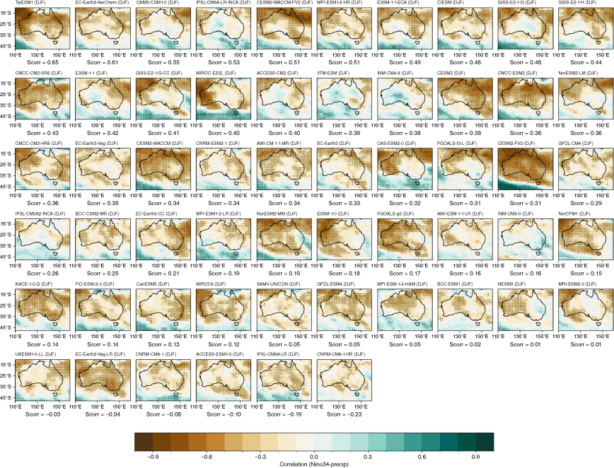
Correlation between MAM Niño3.4 index and MAM rainfall for available CMIP6 models, sorted by spatial correlation with observed N3.4–rainfall correlation patterns. Stippling indicates significance at the 90% confidence level according to a t-test.
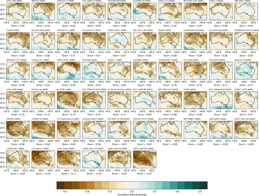
Negative Niño3.4–rainfall correlation
Correlation between DJF Niño3.4 index and DJF rainfall for available CMIP6 models for negN3.4 years only. For this study, negN3.4 years are classified as years when DJF Niño 3.4 < 0. Models are sorted by spatial correlation with observed correlation patterns. Stippling indicates significance at the 90% confidence level according to a t-test.
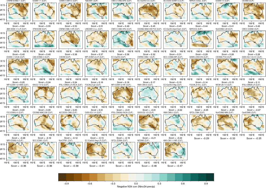
Correlation between MAM Niño3.4 index and MAM rainfall for available CMIP6 models for negN3.4 years only. For this report, neg3.4 years are classified as years when DJF Niño 3.4 < 0. Models are sorted by spatial correlation with observed correlation patterns. Stippling indicates significance at the 90% confidence level according to a t-test.
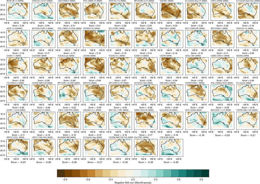
Correlation between JJA Niño3.4 index and JJA rainfall for available CMIP6 models for negN3.4 years only. For this study, negN3.4 years are classified as years when DJF Niño 3.4 < 0. Models are sorted by spatial correlation with observed correlation patterns. Stippling indicates significance at the 90% confidence level according to a t-test.
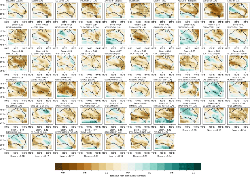
Correlation between SON Niño3.4 index and SON rainfall for available CMIP6 models for negN3.4 years only. For this study, negN3.4 years are classified as years when DJF Niño 3.4 < 0. Models are sorted by spatial correlation with observed correlation patterns. Stippling indicates significance at the 90% confidence level according to a t-test.
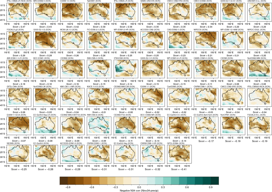
El Niño–rainfall correlation
Correlation between DJF Niño3.4 index and DJF rainfall for available CMIP6 models for posN3.4 years only. For this report, posN3.4 years are classified as years when DJF Niño 3.4 > 0. Models are sorted by spatial correlation with observed correlation patterns. Stippling indicates significance at the 90% confidence level according to a t-test.
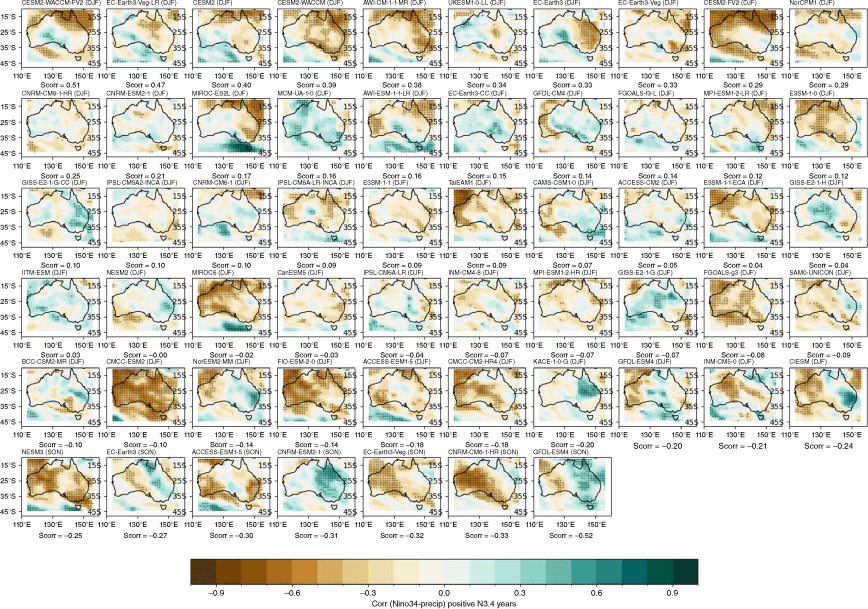
Correlation between MAM Niño3.4 index and MAM rainfall for available CMIP6 models for posN3.4 years only. For this report, posN3.4 years are classified as years when DJF Niño 3.4 > 0. Models are sorted by spatial correlation with observed correlation patterns. Stippling indicates significance at the 90% confidence level according to a t-test.
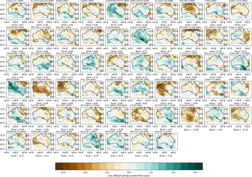
Correlation between JJA Niño3.4 index and JJA rainfall for available CMIP6 models for posN3.4 years only. For this report, posN3.4 years are classified as years when DJF Niño 3.4 > 0. Models are sorted by spatial correlation with observed correlation patterns. Stippling indicates significance at the 90% confidence level according to a t-test.
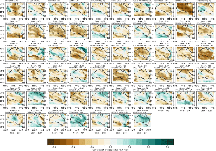
Correlation between SON Niño3.4 index and SON rainfall for available CMIP6 models for El Niño years only. For this report, El Niño years are classified as years when DJF Niño 3.4 > 0. Models are sorted by spatial correlation with observed correlation patterns. Stippling indicates significance at the 90% confidence level according to a t-test.
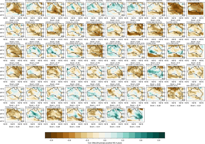
IOD–rainfall correlation
SAM–rainfall correlation
Correlation between DJF rainfall and the DJF SAM index in each CMIP6 model, sorted by spatial correlation with observations. Stippling indicates significance at the 90% confidence level according to a t-test.
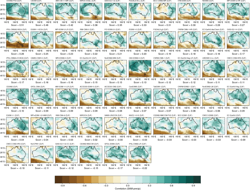
Correlation between MAM rainfall and the MAM SAM index in each CMIP6 model, sorted by spatial correlation with observations. Stippling indicates significance at the 90% confidence level according to a t-test.
