Biases and teleconnections in the Met Office Global Coupled Model version 5.0 (GC5) – insights for seasonal prediction and Australia
Chen Li A * , Debra Hudson
  A , Xiaobing Zhou
  A , Hongyan Zhu
  A , Matthew C. Wheeler
  A , Griffith Young
  A , Charline Marzin B and Luke Roberts B
A
B
Abstract
The Australian Bureau of Meteorology (The Bureau) has been involved in the package testing and assessment process of the UK Met Office Global Coupled Model Version 5.0 (GC5) configuration. GC5 will underpin the Met Office’s next seasonal prediction system, global coupled numerical weather prediction (NWP) system and Earth System Model. It will also likely be the next version of The Bureau’s seasonal prediction system, and the version to replace the global atmosphere-only NWP system to be the first global coupled NWP system at The Bureau. The GC5 configuration includes a new sea-ice model and substantial updates to almost all areas of model physics. We have evaluated the present-day climate simulation, and compared it to observations and with previous versions GC4 and GC2. Our assessment focuses on the climate mean state and variabilities relevant to Australian seasonal prediction, including the El Niño–Southern Oscillation (ENSO), the Indian Ocean Dipole (IOD), the Southern Annular Mode and the Madden–Julian Oscillation. Notably, in comparison to its predecessor (GC4), GC5 shows significant improvements in the eastern Pacific mean state but a slight degradation in the Indian Ocean in terms of the mean state and variability. These and other results provide us with early insights of the potential performance of the next sub-seasonal or seasonal forecast system. Longstanding issues in the seasonal prediction system associated with the equatorial eastern Indian Ocean biases and an overactive ENSO and IOD will likely remain; however, improvements over the eastern equatorial Pacific in GC5 hold promise of improved prediction skill of ENSO and its teleconnections.
Keywords: Australian seasonal prediction, climate drivers, El Niño–Southern Oscillation, ENSO, Indian Ocean Dipole, IOD, Madden–Julian Oscillation, mean state biases, MJO, model evaluation, UK Met Office Global Coupled Model.
1.Introduction
The latest UK Met Office (UKMO) Global Coupled (GC) Model is GC version 5.0 (GC5). The configuration was frozen in May 2022 and was released in mid-2023. The Australian Bureau of Meteorology (The Bureau) has been involved in the package testing and assessment phase of GC5 development, making this the first time that The Bureau has contributed to the evaluation of model performance before a major GC release. GC5 will underpin the UKMO’s next seasonal prediction system (GloSea), their global coupled Numerical Weather Predication (NWP) system, and their Earth System Model (UKESM2). The Bureau’s next seasonal prediction system will also likely use GC5. The current operational seasonal forecast system (ACCESS-S2; Wedd et al. 2022) is based on the much earlier version, GC2, which was frozen in May 2010.
GC5 includes a Global Atmosphere and Land model (GAL9) coupled to a Global Ocean and Sea Ice model (GOSI9) (Xavier et al. 2023). Compared to its predecessor, GC4 (which was frozen in March 2020), GC5 has had major updates to all components of the coupled model and coupling system. This includes a new sea ice model (the Sea Ice-modelling Integrated Initiative, SI3, which replaced the CICE model) (Aksenov et al. 2019) and a major upgrade of the ocean model. There are also substantial updates to the atmospheric physics, in particular the convection, large-scale cloud and gravity wave drag schemes, as well as moderate changes to most other physics schemes. In terms of the coupling changes, GC5 uses a new river runoff coupling scheme, which improves the locations of freshwater runoff into the ocean. GC5 also allows solar radiation to penetrate into the sea ice in the coupled model, which reduces excessive top melt. For more detailed updates from GC4 to GC5 please refer to Xavier et al. (2023).
Currently, The Bureau’s evaluation of GC5 for climate timescales has been focused on the free-coupled climate run, since the seasonal hindcasts are not yet available. This study assesses the coupled model’s mean state biases, key large-scale climate drivers and their teleconnections to the Australian region, to provide insights into the model’s general performance and potential implications for seasonal prediction. The key climate drivers addressed include the El Niño–Southern Oscillation (ENSO), Indian Ocean Dipole (IOD), Madden–Julian Oscillation (MJO) and Southern Annular Mode (SAM).
2.Model and methods
2.1. GC models
GC5 comprises the Global Atmosphere and Global Land configuration GAL9.0, and the Global Ocean and Global Sea Ice configuration GOSI9.0, and they are coupled using the OASIS3-MCT coupler. The code base for GAL9.0 is UM (Unified Model) version 12.2 and JULES (Joint UK Land Environment Simulator) version 6.3. For GOSI9.0, the code is based on NEMO (Nucleus for European Modelling of the Ocean) version 4.0 and SI3 version 4.0 (Table 1). We analysed several GC5 configurations during the package testing phase (before the configuration was frozen), including both N96 and N216 resolutions. Results presented here are based on the frozen release candidate version 4 (GC5-rc4). It is a present-day free coupled run for a total of 100 years, which uses constant (year 2000) greenhouse gas and aerosol concentrations. The model runs at N216 horizontal resolution (~60 km) for atmosphere and land and 0.25° (ORCA025) resolution for ocean and sea ice. There are 85 vertical levels in the atmospheric model; 4 soil levels and multiple snow layers in the land model; 75 vertical levels in the ocean model; and 5 ice thickness categories, 4 ice layers and 1 snow layer in the sea ice model. The atmosphere and land surface are initialised from an AMIP spin-up run, and the ocean is initialised from EN4 (Good et al. 2013) climatological ocean temperatures and salinity averaged between 1995 and 2014. Sea ice is initialised from a SI3 restart file made by converting the standard CICE (the previous sea ice model) start dump into the new SI3 format. To assess model improvements, GC5-rc4 is compared with the equivalent experiment based on the predecessor configuration, GC4. Results are also compared to GC2’s free-coupled run, as an additional benchmark, given that The Bureau’s current seasonal prediction system uses GC2. Table 1 compares the scientific configuration versions and their corresponding code base for the three GC releases.
| Coupled version | Atmosphere and land version | Ocean and sea ice version | Coupled | Resolutions used here atmosphere–ocean | |||
|---|---|---|---|---|---|---|---|
| GC5.0 | GAL9.0 (UM12.2 &JULES6.3) | GOSI9.0 (NEMO_4.0.4 & SI3_4.0.4) | OASIS3-MCT | N216/ORCA025 | |||
| GC4.0 | GA8.0 (UM11.6) | GL9.0 (JULES5.7) | GO6.0 (NEMO3.6) | GSI8.1 (CICE5.1.2) | OASIS3-MCT | N216/ORCA025 | |
| GC2.0 | GA6.0 (UM8.5) | GL6.0 (JULESum8.5) | GO5.0 (NEMO3.4) | GSI6.0 (CICE4.1.1) | OASIS3 | N216/ORCA025 | |
2.2. Datasets and methods
The model’s sea surface temperature (SST) mean state is evaluated against the NOAA Optimum Interpolation SST (OISST.v2) (Reynolds et al. 2002) for the period 1982–2021, whereas the subsurface temperature is assessed using the WOA18 long-term mean climatology (Locarnini et al. 2018). Evaluation of the model’s monthly mean atmospheric circulations, including precipitation, 10-m horizontal winds and sea level pressure (SLP), is done relative to the ERA5 reanalysis (Hersbach et al. 2019) for the period 1982–2020. Daily data from ERA5 are also used for analysis and evaluation of the MJO and rainfall onset date (variables include precipitation, outgoing longwave radiation (OLR) and zonal wind at 850 and 200 hPa). The final 50 years of model output are used for the evaluation (unless otherwise noted). Note that data for GC2 are only for the atmosphere and for monthly means, whereas there are both atmospheric and oceanic daily data for GC4 and GC5.
The Niño3.4 index, which is calculated by the area-averaged SST anomalies in 5°S–5°N, 170–120°W (Trenberth 1997), is used to measure the ENSO activity. The Indian Ocean Dipole Mode Index (DMI) is defined by the difference in SST anomaly between the tropical western Indian Ocean (WIOD, 10°S–10°N, 50–70°E) and the eastern pole (EIOD, 10°S–equator, 90–110°E) (Saji et al. 1999). We utilise the real-time multivariate MJO index to determine the eight MJO phases. This is computed by projecting the daily OLR and zonal winds at 850 and 200 hPa onto the first two Empirical Orthogonal Functions (EOF) of the combined anomalies (Wheeler and Hendon 2004). The spatial pattern of SAM is represented by the leading EOF mode (EOF1) of the southern hemisphere SLP (Thompson et al. 2000), whereas the SAM index is calculated by the difference of zonal mean monthly SLP between 40°S and 65°S (Gong and Wang 1999). We use the linear regression method to identify the teleconnection between key drivers and Australian climate. In addition, a spectrum analysis is also applied to detect the power distribution of the SST indices and the MJO strength. To explore the independent ENSO and IOD teleconnection, we applied a regression method (e.g. Li et al. 2006) to first detect the IOD-related (ENSO-related) signal, then removed it from the original SST and atmospheric circulation data, and recalculated the teleconnection maps. Note that the process only removes the linear signals between ENSO and IOD. To address the ENSO asymmetry, the SST anomaly skewness is calculated by the normalised third statistical moment:
where mk is the kth moment:
and where xi is the ith value of the sample, X is the mean, and n is the number of samples (e.g. Burgers and Stephenson 1999; An 2009).
3.Mean state and variability biases
3.1. Mean state biases
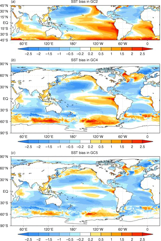
The SST variations in the tropical Pacific and Indian Oceans are important drivers that provide climate predictability on seasonal timescales. Fig. 1 shows the annual mean climatology SST bias. Note that for GC2 the SST is represented by surface temperature from the atmosphere model, and it is not accurate over sea ice, thus only lower latitudes are displayed for GC2. One noteworthy model improvement is in the tropical eastern Pacific, where the warm bias has been significantly reduced in GC5-rc4. The Southern Ocean warm bias has also been improved from GC4 to GC5-rc4. However, the cold SST bias in the tropical eastern and south-eastern Indian Ocean remains and is slightly degraded in GC5-rc4. In general, GC5-rc4 shows a cold SST bias across most of the southern hemisphere.
Annual mean SST (°C) climatology bias (against the NOAA OI SST) for (a) GC2, (b) GC4, and (c) GC5-rc4.
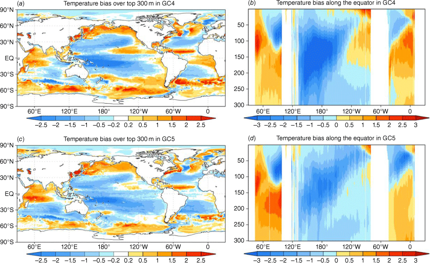
The warm bias in the eastern Pacific prevails from the surface to ~150-m depth in GC4 (Fig. 2a, b). This subsurface warm bias is very much reduced in GC5-rc4 (Fig. 2c, d). The cold subsurface bias in the western and central Pacific has also been improved. In the eastern Indian Ocean, in both models there is a cold bias from the surface down to ~100 m, replaced by a warm bias at deeper levels. This dipole-type subsurface temperature bias in the eastern Indian Ocean is worse in GC5-rc4 (Fig. 2).
Annual mean subsurface temperature (°C) climatology bias (against the WOA18 long-term mean climatology) in (a, b) GC4 and (c, d) GC5-rc4. The maps (left panels) show the averaged top 300-m temperature bias, and the graphs (right panels) show the temperature bias with depth down to 300 m along the equator.
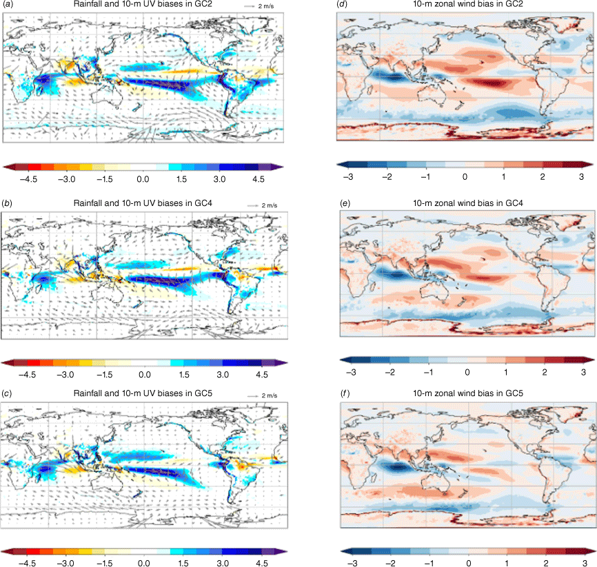
Corresponding to the reduced temperature bias in the eastern Pacific, the associated rainfall bias is decreased in GC5-rc4 compared to both GC4 and GC2 (Fig. 3a–c). Also, GC5-rc4 shows the smallest surface wind bias over the entire tropical Pacific region among the three model configurations (Fig. 3). Over the Indian Ocean, however, the outstanding dry bias in the east and wet bias in the west is persistent across all the models, and is related to the cold and warm SST biases respectively (Fig. 1) and easterlies that are too strong over the tropical Indian Ocean (Fig. 3d–f).
Same as Fig. 1, but for precipitation (shading, mm day−1) and 10-m winds (a–c) (vectors, m s−1) and 10-m zonal wind (d–f). The biases are measured against the ERA5 reanalysis.
In summary, there are notable model improvements in the eastern Pacific region, in terms of the mean temperature state in both surface and subsurface, the precipitation, as well as the surface wind. However, the tropical Indian Ocean mean state biases remain, characterised by the cold (warm) and dry (wet) bias in the east (west) along with easterly winds that are too strong. These mean state biases in the tropical Indian Ocean have been present in all previous GC versions and shown up in the seasonal prediction systems of the UKMO (GloSea), The Bureau (ACCESS-S) and ECMWF (SEAS5). A working group, the Unified Model Partnership’s Indo-Pacific Priority Evaluation Group, was formed in 2020 which aims to understand and improve these biases.
3.2. Biases in SST variability
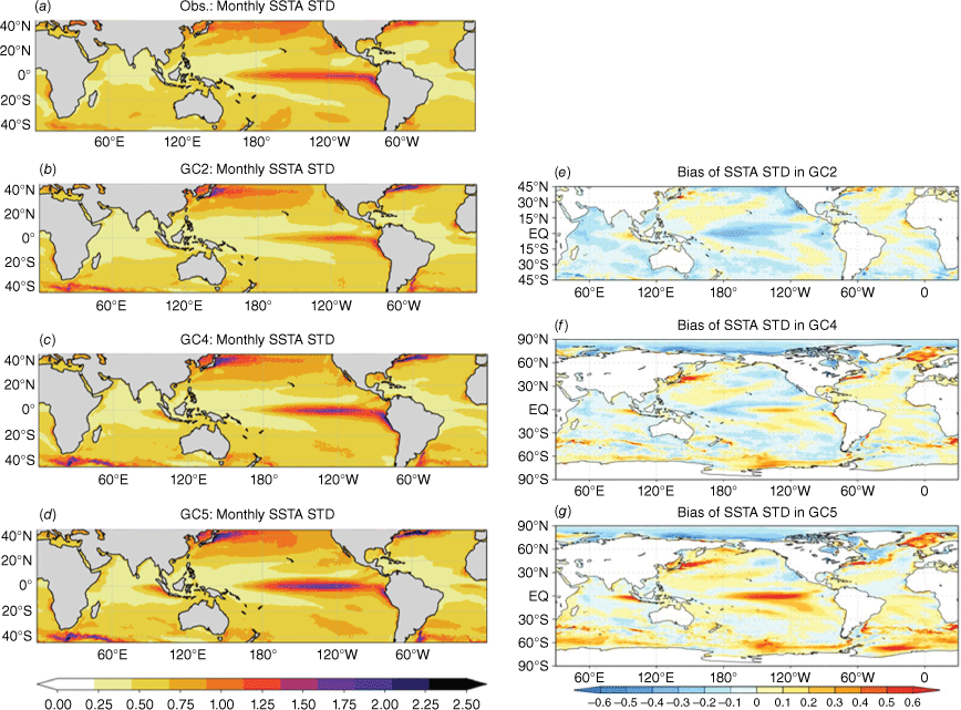
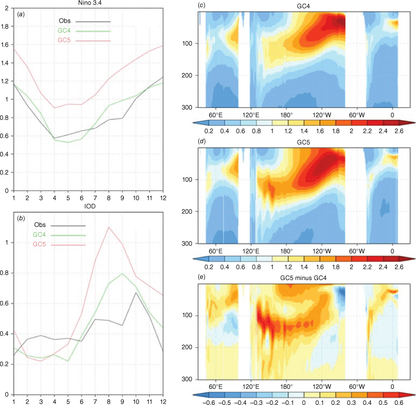
Although the SST bias in the eastern Pacific is reduced in GC5-rc4, the variability of monthly SST anomalies (SSTa) in the central to eastern equatorial Pacific is stronger in GC5 compared to GC4, GC2 and observed (Fig. 4). The three model configurations act very differently in the Pacific Ocean. GC2 underestimates the variability across the central to eastern Pacific. GC4 shows weaker-than-observed variability in the central Pacific but stronger-than-observed in the east. The SSTa variability in the central to eastern Pacific is overestimated in GC5-rc4. The maximum SST variability centre seems to be shifted westward in successive models. In observations, the strongest variability is found in the Niño1 + 2 region. In GC4, the variability in Niño3 region is stronger than observed, and this is worse in GC5 and extends westward to the Niño3.4 region (Fig. 4a–d). For the Niño3.4 region, GC5 has stronger SSTa variability throughout the seasonal cycle (Fig. 5a). The power spectrum of the Niño3.4 index suggests that the frequency distribution of GC5’s variability is too strong and peaks at ~40 months (Fig. 6c). It is interesting to note that the strong 2–3 years ENSO variability is mostly focused in the last three decades of the model output (Fig. 6d). Thus, the ENSO variability shows pronounced decadal changes in GC5-rc4. In general, GC4 seems to show the smallest monthly SST variability bias in the tropical Pacific region (Fig. 4f).
(a–d) The observed (NOAA OI SST) and simulated SST anomalies standard deviation. Bias in the standard deviation of monthly SST anomalies (°C) for (e) GC2, (f) GC4, and (g) GC5-rc4.
Variability (standard deviation; STD) of monthly mean ocean temperature anomalies (°C). The left panels show the seasonal cycle of SSTa variability for the (a) Niño3.4 region and (b) IOD from observations (black), GC4 (green), and GC5-rc4 (red). The right panels show the annual mean STD of monthly temperature anomalies with depth down to 300 m along the equator from (c) GC4, (d) GC5, and (e) the difference between the two.
Power spectra for the Niño3.4 index in (a) GC2, (b) GC4, and (c) GC5-rc4. The observed result is displayed in grey lines. The red lines indicate the upper (95%) confidence bound for the red-noise spectra. (d) The time series of the Niño3.4 index for the last 70 model years from GC5. (e–h) The same as (a–d), but for the eastern pole of the Indian Ocean Dipole (E_IOD).
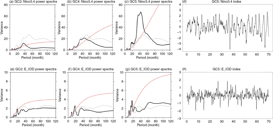
For the Indian Ocean, the weak SSTa variability bias in the western tropical region has been improved, but the overactive eastern Indian Ocean is worsened in GC5-rc4 (Fig. 4e–g). GC5 has too strong biennial variability in the tropical eastern Indian Ocean (Fig. 6g). The variability of the IOD is also stronger than observed in GC5 (and stronger than GC4) for times of the year that the IOD is active (Fig. 5b).
The variability of ocean temperature anomalies with depth along the equator is greater in GC5-rc4 than GC4, particularly along the thermocline (Fig. 5c–e). Although it is not clear whether this variability increase in GC5 is attributable to changes to the ocean model or atmosphere model, it is likely that atmosphere–ocean coupling results in positive feedbacks, given that the shallower thermocline and stronger winds exist to some extent in the respective component-only models (not shown).
To address the relative strength of La Niña and El Niño events, Fig. 7 shows the SST anomaly skewness. In observations there is a strong positive region in the eastern Pacific, indicating that El Niño events are stronger than La Niña events (as has been shown previously, e.g. An 2009). Neither GC2 nor GC4 capture the observed pattern of skewness, showing near-normal distributions of SST anomalies in the eastern equatorial Pacific. GC5 shows marked improvements in SST anomaly skewness compared to GC2 and GC4. The improved skewness in the eastern Pacific is clear, although the positive region does not extend far enough to the north and west compared to observed. In addition, GC5 somewhat overemphasises the negative skewness in regions of the warm pool in the western Pacific.
4.Key climate drivers and their teleconnections
4.1. El Niño–Southern Oscillation (ENSO)
ENSO is a major driver of Australian winter–spring climate variability and predictability (e.g. Nicholls 1989; Risbey et al. 2009). El Niño years are associated with cooler-than-usual SST around Australia and substantially decreased convection over the Maritime Continent region (e.g. Ropelewski and Halpert 1987). This typically leads to reduced winter–spring rainfall across much of Australia, particularly the northern and eastern region (e.g. Risbey et al. 2009; Fig. 8a). During La Niña years, the strengthened Pacific trade winds tend to push moist air into the western Pacific, bringing higher-than-average rainfall over eastern and northern Australia (e.g. Chung and Power 2017).
The regression map of rainfall (shading, mm day−1) and 10-m winds (vectors, m s−1) respectively onto the normalised Niño3.4 index during austral winter and spring (JJA + SON) in (a) ERA5, (b) GC2, (c) GC4, and (d) GC5-rc4. The dots indicate significance at the 5% level for the rainfall regression. Only the significant winds (at the 5% level) are shown in the plots. Seventy years of model outputs are used for the regression map.
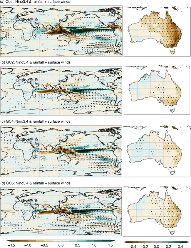
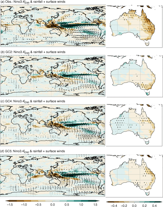
In all three model configurations, the relationship of Niño3.4 with rainfall and 10-m winds is significantly weaker over the tropical Pacific region, especially over the Maritime Continent region compared to observed (Fig. 8), and the rainfall signal associated with ENSO over the tropical eastern Indian Ocean is shifted too far west. In general, the models can capture the ENSO–Australian rainfall teleconnection pattern, albeit the magnitude is weaker than the observed. The weaker convection response over the Maritime Continent region may be contributing to the weak ENSO–Australia rainfall relationship in the model compared to the observed. Among the three model configurations, GC5-rc4 displays the best and strongest ENSO–Australia teleconnections with increased magnitude and more significant areas in eastern Australia (Fig. 8b–d). The enhanced ENSO–Australia teleconnection may be partially related to the strengthened ENSO variability in GC5 (e.g. Cai et al. 2021).
The ENSO teleconnection to southern regions of Australia comes mostly by Rossby waves emanating from the tropical Indian Ocean (Cai et al. 2011). This means that the persistent mean biases in the tropical Indian Ocean are likely limiting the improvement of the ENSO teleconnection to southern Australia despite the mean state improvements within the tropical Pacific region (Fig. 1 and 3). The influence of the Indian Ocean on the ENSO teleconnection to Australian climate is discussed further in the next subsection.
It is worth noting that both GC2 and GC4 show a significant negative relationship with the Niño3.4 index in north-western Australia, which is opposite to the observed. This teleconnection bias has been corrected in GC5-rc4.
4.2. Indian Ocean Dipole (IOD)
The IOD is another key driver of Australian climate variability on monthly to seasonal timescales (e.g. Ashok et al. 2003; Cai et al. 2011). The IOD usually starts to develop in May–June, peaks during August–October, then rapidly decays around the end of austral spring when the Australian summer monsoon arrives (e.g. Zhao and Hendon 2009). The positive phase of the IOD, which is marked by a warm SST anomaly in the tropical western Indian Ocean and a cold anomaly in the tropical eastern Indian Ocean (Saji et al. 1999), typically brings less rainfall over central, eastern and southern Australia, and vice versa for a negative event (e.g. Risbey et al. 2009).
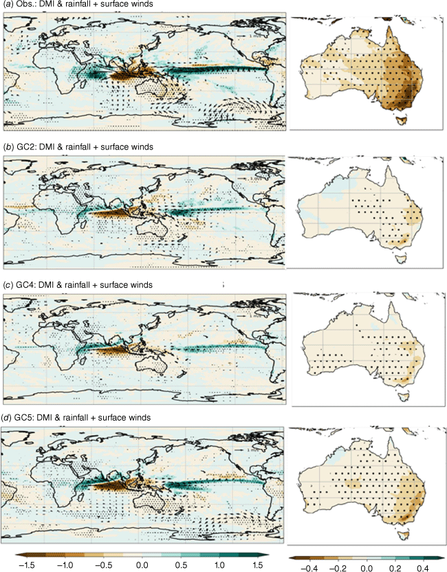
Similar to the ENSO teleconnection, the GC models underestimate the convection anomaly associated with the IOD over the Maritime Continent region, as well as the IOD teleconnection to Australian winter–spring rainfall (Fig. 9). It is worth noting that the IOD-teleconnection pattern is similar to that of ENSO due to their strong covariability especially in austral spring (e.g. Luo et al. 2010). The independent ENSO and IOD teleconnection will be addressed later. The eastern pole of the dipole rainfall anomaly pattern in the tropical Indian Ocean extends too far west in the GC models. This may be partially caused by the strong easterly mean state bias over the tropical Indian Ocean in GC models (Fig. 3d–f). Besides, the relationship between the IOD and the winds over the central Indian Ocean basin is too weak in the GC models (Fig. 9). There is an improved IOD–extratropical wind teleconnection in GC5-rc4 over the southern Indian and Pacific Oceans (Fig. 9d). Previous studies (e.g. McIntosh and Hendon 2018; Goyal et al. 2021) have suggested that deep tropical convection over the Indian Ocean can generate these extratropical variations through Rossby wave trains. Investigation of the propagation of these Rossby waves in the models will be a subject of future work. GC5-rc4 also shows the strongest (improved) IOD–Australian rainfall teleconnection among the three model configurations (Fig. 9d), even though the Indian Ocean mean state is slightly degraded compared to GC2 and GC4 (Fig. 1 and 3). The IOD teleconnection to southern Australia is likely too weak in all the models due to the biases in the tropical Indian Ocean that are influencing the Rossby wave teleconnection to southern Australia (e.g. McIntosh and Hendon 2018).
Same as Fig. 8 during austral winter and spring (JJA + SON) in (a) ERA5, (b) GC2, (c) GC4, and (d) GC5-rc4, but for the Indian Ocean Dipole Mode Index (DMI) regression.
Both ENSO and the IOD are not totally independent and can interact with each other through changes in the Walker Circulation, particularly in austral spring (SON) (Behera et al. 2006). In general, all models can simulate the observed positive ENSO–IOD correlation in the spring (SON), although weaker than observed (Table 2). It is intriguing to explore the ENSO teleconnection (IOD teleconnection) with IOD (ENSO) signals removed as done in Cai et al. (2011). Fig. 10 shows the ENSO teleconnection with the IOD signal removed. Removing the influence of the IOD reduces the impact of ENSO on south-eastern Australian rainfall (Fig. 8a and 10a). This is consistent with the previous study by Cai et al. (2011), where they argued that the direct impact of ENSO on Australian rainfall is mainly confined to the near-tropical portions of eastern Australia. The impacts on south-eastern Australian rainfall during ENSO events are suggested to stem from Rossby waves forced by convective variations in the eastern Indian Ocean, for which the IOD is a primary source of variability. Therefore, a weakened ENSO–south-eastern Australian rainfall relationship is to be expected when the IOD signal is removed. This phenomenon is reasonably well captured in GC5-rc4 (Fig. 8d and 10d). By contrast, GC2 continues to show significant ENSO impacts on rainfall in the south-eastern region after the influence of the IOD has been removed, whereas no significant impact is shown in tropical Australia (Fig. 10b). This suggests that GC2 is misrepresenting the ENSO relationship to Australian rainfall.
| C.C | Obs. (~39 years) | GC2 (70 years) | GC4 (70 years) | GC5 (70 years) | |
|---|---|---|---|---|---|
| ENSO & IOD (SON) | 0.59 | 0.42 | 0.27 | 0.36 | |
| ENSO & SAM (DJF) | −0.29 | 0.11 | 0.10 | −0.26 |
Data in bold are significant at the 90% level.
Same as Fig. 8 during austral winter and spring (JJA + SON) in (a) ERA5, (b) GC2, (c) GC4, and (d) GC5-rc4, but with IOD-related signal removed.
The IOD teleconnection without the ENSO signal is displayed in Fig. 11. The strongest impact of the IOD on Australian winter–spring rainfall is shown in the south-eastern region (Fig. 11a). This teleconnection pattern is noticeably improved in GC5-rc4 (Fig. 11d) compared to both GC2 and GC4 (Fig. 11b, c).
Same as Fig. 9 during austral winter and spring (JJA + SON) in (a) ERA5, (b) GC2, (c) GC4, and (d) GC5-rc4, but with ENSO-related signal removed.
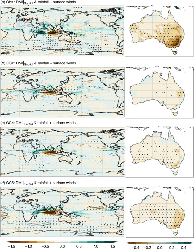
In summary, analysis of the ‘pure’ ENSO and IOD teleconnections indicate that GC5-rc4 is the best in simulating ENSO and IOD impacts on Australian rainfall among the three model configurations.
4.3. Madden–Julian Oscillation (MJO)
The MJO is the dominant mode of tropical variability on sub-seasonal timescales. Previous studies also addressed the importance of the MJO to other modes of variability such as ENSO (e.g. Hendon et al. 2007a), North Atlantic Oscillations (e.g. Zhang 2013) and tropical cyclones (e.g. Camargo et al. 2009). For instance, the MJO can modulate the large-scale conditions associated with the Australian summer monsoon (Wheeler and McBride 2005); strong MJO events can lead to the formation and intensification of tropical cyclones (Camargo et al. 2009; Klotzbach 2014); and the MJO can influence ENSO through the westerlies anomalies associated with the MJO’s eastward propagation (Hendon et al. 2007a). Thus, a well-represented MJO is essential for variability on a range on timescales, from days to seasons.
It is still a challenge for the state-of-the-art global coupled models to simulate the MJO. Most of the current CMIP models underestimate the MJO amplitudes, especially as related to OLR, and struggle to generate a coherent eastward propagation (Ahn et al. 2017). Fig. 12 shows the frequency–wavenumber analysis for observations and GC4 and GC5 models for periods of 10–90 days. The MJO activity is focused around zonal wavenumbers 1–3 and the 30–80-day period (Fig. 12a). The GC models experience common model issues with a weaker-than-observed MJO amplitude and a shorter active period (Jiang et al. 2015; Fig. 12). GC5-rc4 is worse than GC4 with a lack of longer-period (i.e. 35–80 days) wave activity (Fig. 12c). The shorter activity period may indicate that the simulated MJO propagates too fast, or that it cannot propagate far enough into the western hemisphere compared to observations. The poor propagation may be partially related to the reduced meridional moisture gradient in the Maritime Continent region (e.g. Kang et al. 2021), which is contributed by the underlying model dry bias in the southern Maritime Continent (Fig. 3a–c). Fig. 13 compares the MJO eastward propagation in observations and the models. This is represented by composites of the near-equatorial (10°S–10°N) OLR anomalies according to the eight MJO phases derived from the real-time multivariate MJO index (Wheeler and Hendon 2004). The underestimated magnitude of the MJO is worse in GC5-rc4, especially for the central Indian Ocean region. In addition, MJO activity diminishes rapidly after the convection has moved over the Maritime Continent in both models, but more so in GC5-rc4 (Fig. 13).
Cross spectra of OLR (shading) and U850 wind (vectors): coherence-squared and phase relationships in wave number frequency space in (a) ERA5 (1989–2008), (b) GC4, and (c) GC5 (last 20 years for the model output). Upward-pointing arrows indicate an in-phase relationship, downward-pointing an out-of-phase relationship and arrows pointing to the left indicate that negative OLR is leading positive zonal wind by a quarter cycle.

MJO phase–longitude plot for the near-equatorial (10°S–10°N) OLR anomalies (W m–2) for (a) ERA5, (b) GC4, and (c) GC5. The red dashed vertical line indicates the location of 150°E (which is approximately the eastern border of the Maritime Continent). The total days used for the composite for each phase (i.e. phases 1–8) is shown in parentheses.

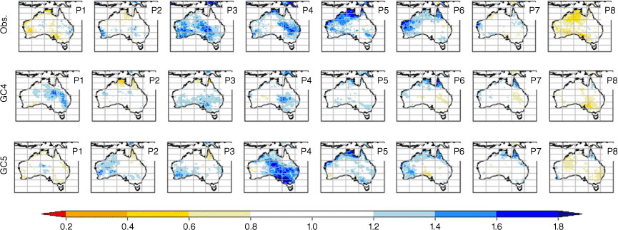
The MJO has its strongest impact on northern Australia in summer (DJF). The northern Australian rainfall response is a result of the direct impact of the MJO’s tropical convection anomalies (Wheeler et al. 2009). Thus, the biggest MJO-related rainfall anomaly occurs when the MJO moves from the Maritime Continent to the western Pacific (phases 5 and 6). Interestingly, the GC5-rc4 shows an improved (stronger) rainfall response in phase 5 (Fig. 14), even though the MJO signal is generally weaker in GC5-rc4 (compared with GC4) (Fig. 12). Further analysis is needed to explore the underlying reasons.
MJO phase composites of weekly rainfall probabilities (exceeding the upper tercile) in austral summer (DJF) in ERA5 (top row), GC4 (middle) and GC5 (bottom row). The values show a ratio of the conditional probability of exceeding the upper tercile relative to the climatological probability of exceeding that threshold, which is normally 33%. Values greater than 1.0 therefore indicate a higher-than-normal chance of exceeding the threshold in that MJO phase.
4.4. Southern Annular Mode (SAM)
The SAM is the leading mode of the extratropical circulation variability in the southern hemisphere throughout the year (e.g. Thompson and Wallace 2000). It refers to the non-seasonal north–south movement of the westerlies in the mid to high latitudes (Hartmann and Lo 1998). This strong westerly band is normally associated with storms and cold fronts that move from west to east (Gillett et al. 2006). All the GC models can well capture the SAM pattern, with correlation coefficients between the observed and the simulated SAM pattern (EOF1) all over 0.98 (Fig. 15). However, the models tend to generate stronger SAM variability than the observed, and this is slightly worse in GC5-rc4 (Fig. 15d). In particular, the centre of maximum variability east of the dateline is overestimated in GC5-rc4 and positioned slightly too far west (Fig. 15d).
The first EOF mode of monthly SLP anomalies across the whole year for (a) ERA5, (b) GC2, (c) GC4, and (d) GC5-rc4. The percentage explained variance is indicated in the right upper corner. The model’s pattern correlation and averaged standard deviation ratio against observed is also shown above each map.

The impacts of SAM on Australian rainfall vary by season. Fig. 16 shows the SAM impacts on Australia by regressing the rainfall anomaly onto the monthly SAM index. During austral summer (DJF), a positive phase of SAM (westerlies contract towards the pole) tends to increase rainfall across most of eastern Australia (including southern Queensland, New South Wales and Victoria) (Fig. 16a) (e.g. Gillett et al. 2006; Hendon et al. 2007b, 2014). The SAM’s impacts on Australian summer rainfall is weaker-than-observed in the GC2 (Fig. 16b), whereas both GC4 and GC5-rc4 show a stronger-than-observed rainfall relationship over eastern Australia (Fig. 16c, d).
The regression map of rainfall (shading, mm day–1) onto the monthly SAM index during summer for (a) ERA5, (b) GC2, (c) GC4, and (d) GC5-rc4. The dots indicate significance at the 5% level for the rainfall anomaly. (e–h) same as (a–d) but for the austral winter season (JJA).
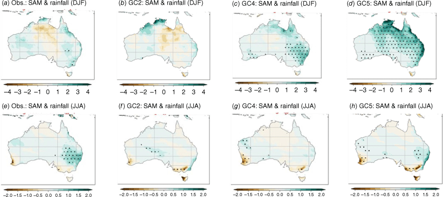
The SAM has been shown to have a negative correlation with ENSO (e.g. L’Heureux and Thompson 2006; Dätwyler et al. 2020). A shift towards more El Niño-like conditions coincides with weaker mid-latitude westerlies, an equatorward shift of the storm tracks and a more negative phase of the SAM (e.g. Lim et al. 2013). Table 2 shows that, unlike GC2 and GC4, GC5 is able to capture this correlation. It is interesting to note that a strong significant region is shown over tropical Australia in GC5-rc4 (Fig. 16d), which might be related to the strong SAM–ENSO teleconnection present in GC5, and not seen in either GC2 and GC4 (Table 2). This correlation although similar to observed, together with an overactive ENSO in GC5, might be causing the stronger than observed teleconnection over northern Australia. This will need to be investigated further in future studies.
During winter (JJA), a positive SAM is associated with increased rainfall over eastern Australia but decreased rainfall in the south-west and the south-east, including Victoria and Tasmania (Fig. 16e) (e.g. Hendon et al. 2007b; Risbey et al. 2009). All the GC models can represent the reduced rainfall in south-western and south-eastern Australia, but only GC5-rc4 shows the significant increase in rainfall over eastern Australia (Fig. 15f). In summary, GC5-rc4 shows an improved SAM–eastern Australia winter rainfall teleconnection.
5.Assessment of a user-oriented metric – the northern rainfall onset
Finally, we assessed one of The Bureau’s user-oriented seasonal climate outlook products, the northern rainfall onset (http://www.bom.gov.au/climate/rainfall-onset). User-oriented metrics are not typically evaluated in routine model development and evaluation assessments. However, apart from obtaining additional insight into model performance, it is beneficial to be able to demonstrate to users the impact of model developments on aspects that are directly relevant to them and helps convey the value to users (and potentially funders) of this fundamental research and development.
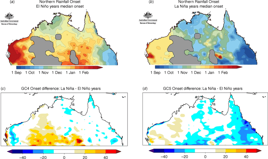
This product was developed in consultation with the northern livestock industry. It is the date at which an accumulation of 50 mm of rain is reached after 1 September and represents the approximate time when new pasture growth starts after the dry season (Drosdowsky and Wheeler 2014; Cowan et al. 2020). The usual onset date is earlier on the east and north coast (the threshold reached prior to November) and later inland and to the west, with onset dates in January and February. However, the onset date is strongly modulated by ENSO. During La Niña (El Niño) years an earlier (later) than usual onset is expected. The difference in onset dates between La Niña and El Niño periods can be as much as 1–2 months (Lo et al. 2007; Fig. 17a, b). The difference in onset time between La Niña and El Niño years in the GC models is shown in Fig. 17. GC4 fails to capture ENSO’s impact on the northern rainfall onset, with no clear difference between the negative and positive phases of ENSO. By contrast, GC5-rc4 is able to reproduce the earlier onset dates in La Niña years for eastern Australian regions.
(a, b) The median northern rainfall onset date for El Niño and La Niña years (obtained from northern rainfall onset outlook, see http://www.bom.gov.au/climate/rainfall-onset/#tabs=Normal-onset). The simulated difference of the northern rainfall onset time between La Niña and El Niño years in (c) GC4 and (d) GC5-rc4 (days). Blue (red) refers to an early (a late) onset.
6.Summary
In this study, we evaluated a present-day climate simulation from the latest global coupled (GC) model configuration from the UKMO. This assessment forms part of the evaluation which led to the formal release of GC version 5 (GC5) in mid-2023. The analysis focuses on mean state biases and the key climate drivers of variability and predictability of Australian climate, including their teleconnections.
The GC5 model will likely be used in The Bureau’s next seasonal prediction system upgrade. The current prediction system, ACCESS-S2 (Wedd et al. 2022), uses a much earlier version of the coupled model, GC2. Seasonal prediction requires the generation of a large set of hindcasts or reforecasts, which are costly and take considerable time to produce. As such, they are not yet available for GC5. Analysis of a free-running coupled model simulation provides us with early insights into the possible performance of GC5 for seasonal prediction.
The GC5 present-day climate simulation has a horizontal resolution of ~60 km (N216) for the atmosphere and 0.25° for the ocean. Comparisons with equivalent simulations from previous model versions, i.e. GC4 and GC2 (used for ACCESS-S2), show that the major improvements in GC5 include the following:
The warm SST bias in the tropical eastern Pacific has been largely reduced in GC5, together with improved surface wind and precipitation mean states in the eastern Pacific.
The warm bias in Southern Ocean SSTs is reduced in GC5.
There are improved (stronger) ENSO–IOD teleconnections to Australian winter–spring rainfall in GC5.
There is an improved relationship between the SAM and eastern Australian winter rainfall in GC5.
There is an improved ability to simulate the modulation of the northern Australian rainfall onset as a function of ENSO in GC5.
However, some longstanding issues of GC models remain in GC5, such as the following:
The cold SST bias in the tropical eastern Indian Ocean is slightly degraded in GC5, which is accompanied by easterly winds that are too strong and a dipole of rainfall biases (too wet in the west and too dry in the east). These mean state biases have been present in all previous GC versions and are a key focus of the Unified Model Partnership’s Indo-Pacific Priority Evaluation Group.
ENSO and the IOD are overactive in GC5, with too strong SST variability in the eastern Pacific and the Indian Ocean.
The MJO is still too weak in GC5 (and is weaker than GC4).
The implications for seasonal forecasting remain to be seen from initialised hindcasts, but results suggest that we may see somewhat improved ENSO forecasts and teleconnections associated with reduced eastern tropical Pacific SST and wind biases. However, it is unclear how the increased variability in the central to eastern Pacific and eastern Indian Ocean will affect the forecast skill. In addition, the longstanding biases in the eastern Indian Ocean remain a challenge and will likely still limit our ability to predict teleconnections to Australian climate.
Data availability
The model output that supports this study will be shared upon reasonable request to the corresponding author.
Declaration of funding
This work is partially funded by the National Environmental Science Program (NESP) and the Northern Australia Climate Program (NACP). The NACP is funded by Meat and Livestock Australia, the Queensland Government through the Drought and Climate Adaptation Program, and the University of Southern Queensland.
Acknowledgements
Thanks to members of the Coupled Modelling Team (Earth System Modelling Section, Research Program), for their suggestions on this research. We thank Dr Eun-Pa Lim, Dr Andrew Marshall and two anonymous reviewers for their constructive suggestions for the manuscript.
References
Ahn MS, Kim D, Sperber KR, et al. (2017) MJO simulation in CMIP5 climate models: MJO skill metrics and process-oriented diagnosis. Climate Dynamics 49, 4023-4045.
| Crossref | Google Scholar |
An SI (2009) A review of interdecadal changes in the nonlinearity of the El Niño-Southern Oscillation. Theoretical and Applied Climatology 97, 29-40.
| Crossref | Google Scholar |
Ashok K, Guan Z, Yamagata T (2003) Influence of the Indian Ocean dipole on the Australian winter rainfall. Geophysical Research Letters 30, 1821.
| Crossref | Google Scholar |
Behera SK, Luo JJ, Masson S, Rao SA, Sakuma H, Yamagata T (2006) A CGCM study on the interaction between IOD and ENSO. Journal of Climate 19(9), 1688-1705.
| Crossref | Google Scholar |
Burgers G, Stephenson DB (1999) The “normality” of El Niño. Geophysical Research Letters 26(8), 1027-1030.
| Crossref | Google Scholar |
Cai W, van Rensch P, Cowan T, Hendon HH (2011) Teleconnection pathways of ENSO and the IOD and the mechanisms for impacts on Australian rainfall. Journal of Climate 24, 3910-3923.
| Crossref | Google Scholar |
Cai W, Santoso A, Collins M, et al. (2021) Changing El Niño–Southern Oscillation in a warming climate. Nature Reviews Earth & Environment 2, 628-644.
| Crossref | Google Scholar |
Camargo SJ, Wheeler MC, Sobel AH (2009) Diagnosis of the MJO modulation of tropical cyclogenesis using an empirical index. Journal of the Atmospheric Sciences 66, 3061-3074.
| Crossref | Google Scholar |
Chung CTY, Power SB (2017) The non-linear impact of El Niño, La Niña and the Southern Oscillation on seasonal and regional Australian precipitation. Journal of Southern Hemisphere Earth Systems Science 67, 25-45.
| Crossref | Google Scholar |
Cowan T, Stone R, Wheeler MC, Griffiths M (2020) Improving the seasonal prediction of Northern Australian rainfall onset to help with grazing management decisions. Climate Services 19, 100182.
| Crossref | Google Scholar |
Dätwyler C, Grosjean M, Steiger NJ, Neukom R (2020) Teleconnections and relationship between the El Niño–Southern Oscillation (ENSO) and the Southern Annular Mode (SAM) in reconstructions and models over the past millennium. Climate of the Past 16, 743-756.
| Crossref | Google Scholar |
Drosdowsky W, Wheeler MC (2014) Predicting the onset of the north Australian wet season with the POAMA dynamical prediction system. Weather Forecasting 29(1), 150-161.
| Crossref | Google Scholar |
Gillett NP, Kell TD, Jones PD (2006) Regional climate impacts of the southern annular mode. Geophysical Research Letters 33, L23704.
| Crossref | Google Scholar |
Gong DY, Wang WS (1999) Definition of Antarctic Oscillation index. Geophysical Research Letters 26, 459-462.
| Crossref | Google Scholar |
Good SA, Martin MJ, Rayner NA (2013) EN4: quality controlled ocean temperature and salinity profiles and monthly objective analyses with uncertainty estimates. Journal of Geophysical Research: Oceans 118, 6704-6716.
| Crossref | Google Scholar |
Goyal R, Jucker M, Sen Gupta A, Hendon HH, England MH (2021) Zonal wave 3 pattern in the Southern Hemisphere generated by tropical convection. Nature Geoscience 14, 732-738.
| Crossref | Google Scholar |
Hartmann DL, Lo F (1998) Wave-driven zonal flow vacillation in the Southern Hemisphere. Journal of the Atmospheric Sciences 55, 1303-1315.
| Crossref | Google Scholar |
Hendon HH, Wheeler MC, Zhang C (2007a) Seasonal dependence of the MJO–ENSO relationship. Journal of Climate 20(3), 531-543.
| Crossref | Google Scholar |
Hendon HH, Thompson DWJ, Wheeler MC (2007b) Australian rainfall and surface temperature variations associated with the Southern Hemisphere Annular Mode. Journal of Climate 20, 2452-2467.
| Crossref | Google Scholar |
Hendon HH, Lim EP, Nguyen H (2014) Variations of subtropical precipitation and circulation associated with the Southern Annular Mode. Journal of Climate 27, 3446-3460.
| Crossref | Google Scholar |
Hersbach H, Bell B, Berrisford P, Biavati G, Horányi A, Muñoz Sabater J, Nicolas J, Peubey C, Radu R, Rozum I, Schepers D, Simmons A, Soci C, Dee D, Thépaut, JN (2019) ERA5 monthly averaged data on single levels from 1959 to present. Copernicus Climate Change Service (C3S) Climate Data Store (CDS). 10.24381/cds.f17050d7
Jiang X, Waliser DE, Xavier PK, et al. (2015) Vertical structure and physical processes of the Madden–Julian oscillation: exploring key model physics in climate simulations. Journal of Geophysical Research: Atmospheres 120, 4718-4748.
| Crossref | Google Scholar |
Kang D, Kim D, Ahn MS, An SI (2021) The role of the background meridional moisture gradient on the propagation of the MJO over the maritime continent. Journal of Climate 34(16), 6565-6581.
| Crossref | Google Scholar |
Klotzbach PJ (2014) The Madden–Julian Oscillation’s impacts on worldwide tropical cyclone activity. Journal of Climate 27, 2317-2330.
| Crossref | Google Scholar |
Li S, Hoerling MP, Peng S, Weickmann KM (2006) The annular response to tropical Pacific SST forcing. Journal of Climate 19, 1802-1819.
| Crossref | Google Scholar |
Lim EP, Hendon HH, Rashid H (2013) Seasonal predictability of the Southern Annular Mode due to Its association with ENSO. Journal of Climate 26, 8037-8054.
| Crossref | Google Scholar |
Lo F, Wheeler MC, Meinke H, Donald A (2007) Probabilistic forecasts of the onset of the north Australian wet season. Monthly Weather Review 135(10), 3506-3520.
| Crossref | Google Scholar |
Locarnini RA, Mishonov AV, Baranova OK, Boyer TP, Zweng MM, Garcia HE, Reagan JR, Seidov D, Weathers K, Paver CR, Smolyar I (2018) World Ocean Atlas 2018, Volume 1: Temperature. (Ed. A Mishonov) NOAA Atlas NESDIS 81. (US Department of Commerce, National Oceanic and Atmospheric Administration, Silver Spring, MD, USA) Available at https://www.ncei.noaa.gov/sites/default/files/2020-04/woa18_vol1.pdf
L’Heureux M L, Thompson DWJ (2006) Observed relationships between the El Niño–Southern Oscillation and the extratropical zonal-mean circulation. Journal of Climate 19, 276-287.
| Crossref | Google Scholar |
Luo JJ, Zhang R, Behera SK, Masumoto Y, Jin FF, Lukas R, Yamagata T (2010) Interaction between El Niño and extreme Indian Ocean dipole. Journal of Climate 23, 726-742.
| Crossref | Google Scholar |
McIntosh PC, Hendon HH (2018) Understanding Rossby wave trains forced by the Indian Ocean Dipole. Climate Dynamics 50, 2783-2798.
| Crossref | Google Scholar |
Nicholls N (1989) Sea surface temperatures and Australian winter rainfall. Journal of Climate 2, 965-973.
| Crossref | Google Scholar |
Reynolds RW, Rayner NA, Smith TM, Stokes DC, Wang W (2002) An improved in situ and satellite SST analysis for climate. Journal of Climate 15, 1609-1625.
| Crossref | Google Scholar |
Risbey JS, Pook MJ, McIntosh PC, Wheeler MC, Hendon HH (2009) On the remote drivers of rainfall variability in Australia. Monthly Weather Review 137(10), 3233-3253.
| Crossref | Google Scholar |
Ropelewski CF, Halpert MS (1987) Global and regional scale precipitation patterns associated with the El Niño/Southern oscillation. Monthly Weather Review 115, 1606-1626.
| Crossref | Google Scholar |
Saji NH, Goswami BN, Vinayachandran PN, Yamagata T (1999) A dipole mode in the tropical Indian Ocean. Nature 401, 360-363.
| Crossref | Google Scholar | PubMed |
Thompson DWJ, Wallace JM (2000) Annular modes in the extratropical circulation. Part I: month-to-month variability. Journal of Climate 13, 1000-1016.
| Crossref | Google Scholar |
Thompson DWJ, Wallace JM, Hegerl GC (2000) Annular modes in the extratropical circulation. Part II: trends. Journal of Climate 13, 1018-1036.
| Crossref | Google Scholar |
Trenberth KE (1997) The definition of El Niño. Bulletin of the American Meteorological Society 78(12), 2771-2777.
| Crossref | Google Scholar |
Wedd R, Alves O, de Burgh-Day C, et al. (2022) ACCESS-S2: the upgraded Bureau of Meteorology multi-week to seasonal prediction system. Journal of Southern Hemisphere Earth Systems Science 72(3), 218-242.
| Crossref | Google Scholar |
Wheeler MC, Hendon HH (2004) An all-season real-time multivariate MJO index: development of an index for monitoring and prediction. Monthly Weather Review 132, 1917-1932.
| Crossref | Google Scholar |
Wheeler MC, Hendon HH, Cleland S, Meinke H, Donald A (2009) Impacts of the Madden–Julian Oscillation on Australian rainfall and circulation. Journal of Climate 22(6), 1482-1498.
| Crossref | Google Scholar |
Xavier P, Willett M, Graham T, et al. (2023) Assessment of the Met Office Global Coupled model version 5 (GC5) configurations. Report. (Met Office: Exeter, UK) Abstract available at https://centaur.reading.ac.uk/112173/
Zhang C (2013) Madden–Julian oscillation: bridging weather and climate. Bulletin of the American Meteorological Society 94, 1849-1870.
| Crossref | Google Scholar |
Zhao M, Hendon HH (2009) Representation and prediction of the Indian Ocean dipole in the POAMA seasonal forecast model. Quarterly Journal of the Royal Meteorological Society 135, 337-352.
| Crossref | Google Scholar |


