

An assessment of the accuracy of satellite-derived woody and grass foliage cover estimates for Australia
Randall J. Donohue A * and Luigi J. Renzullo B
A
B
Abstract
Understanding the functional role of vegetation across landscapes requires the ability to monitor tree and grass foliage cover dynamics. Several satellite-derived products describe total and woody foliage cover across Australia. Few of these are suitable for monitoring changes in woody foliage cover and only one can currently describe subseasonal dynamics in both woody and grass cover.
(1) To improve the accuracy of woody and grass foliage cover estimates in Australia’s arid environments, around major disturbances and in perennially green pastures. (2) To gain a detailed understanding of the accuracy of woody and grass foliage cover estimates for Australia.
Satellite-derived greenness data were converted to total foliage cover fraction (0.0–1.0), accounting for differences in background soil affects. Total cover was split into component woody and grass cover by using a modified persistent–recurrent splitting algorithm. Results were compared with 4214 field measurements of cover.
Accuracy varied between woody and grassland vegetation types, with total, woody and grass foliage cover having low errors (of ~0.08) and near-zero biases across all woody vegetation types. Across grasslands, errors were higher (up to 0.28), and biases were greater (and negative), with both scaling with foliage density.
Foliage cover was accurately estimated for forested through to sparsely wooded ecosystems. Foliage cover of pure, dense grasslands was systematically underpredicted.
This is the only Australian cover product that can generate temporally dense woody and grass foliage cover data and is invaluable for monitoring vegetation dynamics, particularly across Australia’s mixed tree–grass landscapes.
Keywords: Australia, dynamics, foliage cover, grass, satellite, time-series, vegetation, woody.
Introduction
Trees and grasses play distinct functional roles in almost every process across most of Earth’s landscapes. They separately influence the energy, water, nutrient and carbon cycles (Monteith 1972; Budyko 1974; Jackson et al. 2000); they provide different types of goods for human consumption and wellbeing; they differ in how they generate and shelter biological diversity (Watkinson and Ormerod 2001; Brockerhoff et al. 2017); and they influence how these cycles are best modelled (Ruiz-Vásquez et al. 2023; Cranko Page et al. 2024). Each have different characteristics and time scales in their dynamics, which are driven by both natural processes and by human activity. Better understanding and management of Earth’s landscapes, and prediction of likely outcomes of current actions, requires an ability to quantify the separate and highly-dynamic characteristics of trees and grasses.
Space-borne sensors are currently the only practical technology for monitoring vegetation across large areas, either at fine spatial scales (<100 m grid-cell size) or high temporal frequencies (<annual), or both. Of all the structural attributes of vegetation, leaf area is arguably the most easily and directly observable attribute from space-borne sensors. Thus, most vegetation monitoring is based on greenness metrics or on projected foliage cover. The latter, being a biophysical variable, and one which is directly tied to plant physiology (Larcher 2003), is particularly important. Foliage cover has been defined as the proportion of ground that is covered by green leaves when viewed from directly above (Specht 1970).
In Australia, there have been numerous vegetation cover products generated over the past few decades, each differing in their underlying approaches and in the satellite imagery used in deriving them (Table 1). These products variously describe ground cover, total foliage cover and woody foliage cover. Ground cover products describe the fraction of ground covered by photosynthetically active vegetation (that is, green leaves), non-photosynthetically active material (dead leaves, branches, bark, etc.), and bare ground (Guerschman et al. 2009). The green cover variable of these ground cover products is notionally equivalent to total foliage cover, as defined and generated in this paper.
| Product | Model type | Variable | Imagery | Resolution/ time-step | Error | Reference | |
|---|---|---|---|---|---|---|---|
| Land-cover change | SIP | Forest cover | Landsat | 25 m/annual | 0.02 forest/woodland*, 0.33 sparsely wooded* | Australian National Greenhouse Accounts (2023) | |
| Foliage projective cover – Landsat | SIP | Total foliage cover | Landsat | 25 m/annual | 0.10^ | Department of Environment and Science (2021) | |
| Seasonal fractional cover – CSIRO | SIP | Total foliage cover | MODIS | 500 m/monthly | 0.11^ | Guerschman and Hill (2018) | |
| Seasonal fractional cover – JRSRP | SIP | Total foliage cover | Sentinel-2 | 10 m/quarterly | 0.11^ | Joint Remote Sensing Research Program and Department of Environment and Science (2022) | |
| Monthly blended fractional cover – JRSRP | SIP | Total foliage cover | Landsat/Sentinel-2 | 30 m/monthly | NR | Joint Remote Sensing Research Program and Department of Environment and Science (2021) | |
| Woody vegetation cover | SIP | Woody foliage cover | Landsat | 25 m/annual | 0.07^ | Liao et al. (2020) | |
| Forest-cover change | SIP | Woody foliage cover and forest cover | Landsat | 30 m/annual | 0.01* (no forest cover change) 0.19* (forest cover change) | Hansen et al. (2013) | |
| Woody foliage projective cover (FPC) | SIP | Woody foliage cover | Sentinel-2 | 10 m/biennialA | NR | Collett (2024) | |
| Woody extent and foliage projective cover – SPOT | SIP | Woody foliage cover | SPOT | 5 m/annual | 0.09^ | ||
| Woody vegetation cover | TSD | Woody foliage cover | Landsat | 25 m/10-year average | 0.12* | ||
| Seasonal persistent green cover | TSD | Woody foliage cover | Landsat | 25 m/quarterly | NR | Department of Environment and Science (2022a) | |
| Australian monthly fPAR | TSD | Woody and grass foliage cover | AVHRR | 1 km/monthly | NR | Donohue et al. (2013) | |
| Woody and grass foliage cover | TSD | Woody and grass foliage cover | MODIS | 250 m/16-day | – | This paper |
The model type is either single-image parametric (SIP) or time-series decomposition (TSD). Two types of errors are recorded. Errors for categorical data (or data categorised for validation purposes) are reported here as the average of the producer and user percentage accuracies (denoted with asterisk and given as 1 − accuracy / 100). Errors for continuous data are root mean square errors (denoted with ^ and converted from percentage to fractions where necessary). NR means that errors are not reported. Two products report canopy or forest cover rather than foliage cover. One product (forest-cover change) is a global product.
Total foliage cover is the combination of woody foliage cover and grass foliage cover (where woody cover is the green foliage cover of trees and shrubs). Various models have been developed for separating these two components from total cover, which can be broadly categorised as single-image parametric (SIP) models and time-series decomposition (TSD) models (see Table 1). Both depend on the assumptions that, across Australia, effectively all native woody canopy species are evergreen (Specht and Specht 1999; Bowman and Prior 2005) and that the green foliage of grasses is functionally annual (even if the species is perennial). This means that, at some point during each year, grass foliage cover will be at (or close to) zero, at which time the observed cover can be attributed to woody plants.
Single-image parametric models take the reflectance information present in mid-dry-season images, along with field observations of tree cover, and build parametric models to convert reflectance to cover. By using enough observations across space and through time, the resulting models can be applied continentally and used to assess change. These are single-image models in that they do not utilise the time-series information within the imagery. Examples, listed in Table 1, include the Land Cover Change database (which effectively maps woody foliage cover in classes of 5–19% and 20–100%), which is used in Australia’s National Carbon Inventory (Australian National Greenhouse Accounts 2023). Other examples are the various Foliage Projective Cover datasets generated by different State agencies (all ultimately based on Armston et al. 2009). More recently, several woody cover products have been generated at global-to-regional scales by using both satellite reflectance and radar imagery, and utilising machine learning algorithms trained on large LiDAR, biomass and foliage cover databases (Hansen et al. 2013; Liao et al. 2020; Stewart 2021). The numerous Australian ground cover products available are also derived using SIP models. The value of these models is that they require only one image per year and so can utilise high-resolution (10–30 m) imagery (such imagery is generally too happy at seasonal or finer frequencies to support time-series analyses).
In contrast, woody foliage cover products derived using TSD require temporally dense imagery. Such models fit a curve to the intra-annual minimum values of multi-year total foliage cover data, with techniques varying from down-shifted moving averages (Roderick et al. 1999), moving minimums (Gill et al. 2006; Donohue et al. 2009), seasonal-trend statistical decomposition (Lu et al. 2003), and minimum-weighted splines (Department of Environment and Science 2022a). The need for dense time-series imagery has typically restricted this approach to imagery with weekly-to-monthly frequencies, which implicitly means moderate resolution imagery (≥250 m). One exception is the seasonal woody green product (Department of Environment and Science 2022a), which uses quarterly, 25-m Landsat imagery. The advantage of TSD models is that they are sensitive to subseasonal dynamics in the total cover signal. Perhaps most importantly, this means that the highly dynamic foliage cover of grasses can be estimated (as the difference between total and woody cover).
Products describing forest or canopy cover in Table 1 have the lowest reported errors. This is largely a reflection that these are categorical data (namely forest vs non-forest) and predicting forest presence/absence is a far less demanding task than is predicting woody foliage cover. The estimation of total foliage cover has generally yielded errors in the order of 0.1 (or 10% if cover is reported as percentages), regardless of the models used (Sutton et al. 2022). None of the TSD models have reported accuracies of their woody cover estimates (noting that the product from Gill (2021) used a time-series model, but report only a long-term average). However, Gill et al. (2006) have previously assessed three TSD models and found that they performed similarly, with errors also of around 0.10.
The method for estimating foliage cover presented here has two components; the first converts satellite-derived greenness values into total foliage cover and the second uses a moving-minimum-based TSD model to convert total cover into woody and grass cover. Previous versions of this method (Roderick et al. 1999; Donohue et al. 2009; Donohue et al. 2014; Donohue 2021) have varied both in how total foliage cover was calculated and in how the particular TSD model has been implemented (which is a model called the persistent–recurrent splitting algorithm). There are several known shortcomings of this existing method, which are specifically addressed in this work. One is that woody cover estimates in sparsely vegetated environments are systematically over-estimated (Donohue et al. 2009) and under-estimates (Donohue 2021), depending on the assumptions made about the influence of background soil colour on the derivation of total foliage cover. Another shortcoming is that the moving minimum does not properly capture woody cover dynamics immediately preceding a sudden drop in woody cover (such as is associated with major disturbances such as wildfires). Last, it cannot correctly distinguish between grass and woody cover in dense, temperate grasslands. This is because such grasslands do not have the high seasonal variability in total cover that is required to decompose the total cover signal and, as such, grass cover is erroneously interpreted as woody cover.
The first aim of this paper is to modify the existing woody and grass foliage cover method to improve performance in relation to the three shortcomings outlined above. That is, to improve the accuracy of cover estimates (1) in arid environments (especially woody cover), (2) surrounding major disturbance events, and (3) in perennially green pastures. The second aim of this paper is to quantify the accuracy of total, woody and grass foliage cover estimates for Australia.
Materials and methods
The method outlined here describes how satellite-derived normalised difference vegetation index (NDVI) data can be used to estimate the foliage cover of woody vegetation (trees and shrubs) and of grasses (predominantly grasses, but also forbs and other annuals). It represents an adaptation of previous method versions presented by Donohue et al. (2008) and Donohue et al. (2014), which themselves are based on earlier work of Berry and Roderick (2002), Roderick et al. (1999) and Lu et al. (2003). The method consists of the following steps:
Masking-out clouds and cloud shadows.
Applying a maximum-smoothing algorithm that performs minor gap-filling and noise-filtering.
Converting NDVI to total foliage cover.
Modifying and implementing the TSD model (the persistent–recurrent splitting algorithm).
Here, we use MODIS NDVI imagery as the input imagery and the method is applied to every land-based MODIS pixel time-series.
Input imagery
The input NDVI imagery used is the 250 m resolution, 16-day MOD13Q1 NDVI data (Collection 6.1) (Justice et al. 1998). A time-step of 16 days means that there are 23 periods per year. These data span from January 2001 to December 2023. They have been re-projected to geographic coordinates (longitudes and latitudes), and clipped to the extent 112.0°, −10.0° (upper-left cell centres) and 154.0°, −44.0° (lower-right cell centres).
Cloud masking using MODIS quality flags
The following MODIS-supplied VI Quality Assessment Science Data Sets bit values were used to remove cloud and cloud shadow effects: 2066, 2070, 2517, 3098, 3102, 3106, 3482, 4114, 4118, 35,101, 35,225, 35,293, 35,297, 35,302. These were used in preference to the MODIS-supplied cloud flags because the latter often removed cloud-free pixels around salt lakes and inland ephemeral water bodies.
Maximum-smoothing algorithm
Even with the use of these custom-chosen quality flags and with the 16-day compositing inherent within the MOD13Q1 product, the NDVI imagery still contain some cloud effects. These typically suppress values, causing sudden, and usually temporary, dropouts in the time-series, which are physically unrealistic. The presence of such dropouts in the data are further minimised using a moving-maximum smoothing function (which also performs minor gap-filling and noise-filtering). The initial step in the smoothing is to extend the original NDVI (V′, unitless) time-series backward by 1 year by repeating the first year of data, and forward by 1 year by repeating the last year of data (these added years are removed after the full splitting algorithm has been applied). This ensures there are no edge effects when using moving windows. So, for a time-series spanning from 2001 to 2023, there are 23 years of data with 23 16-day periods each year, yielding a total number of timesteps (n) of 529. After extending the time-series, the new number of time-steps (m) is 575 (that is, n + 46).
The maximum smoothing identifies the maximum NDVI value of the current value and the mean of the two values either side of the current value (so a mean of four values). Thus, the maximum-smoothed NDVI (V) is calculated as follows:
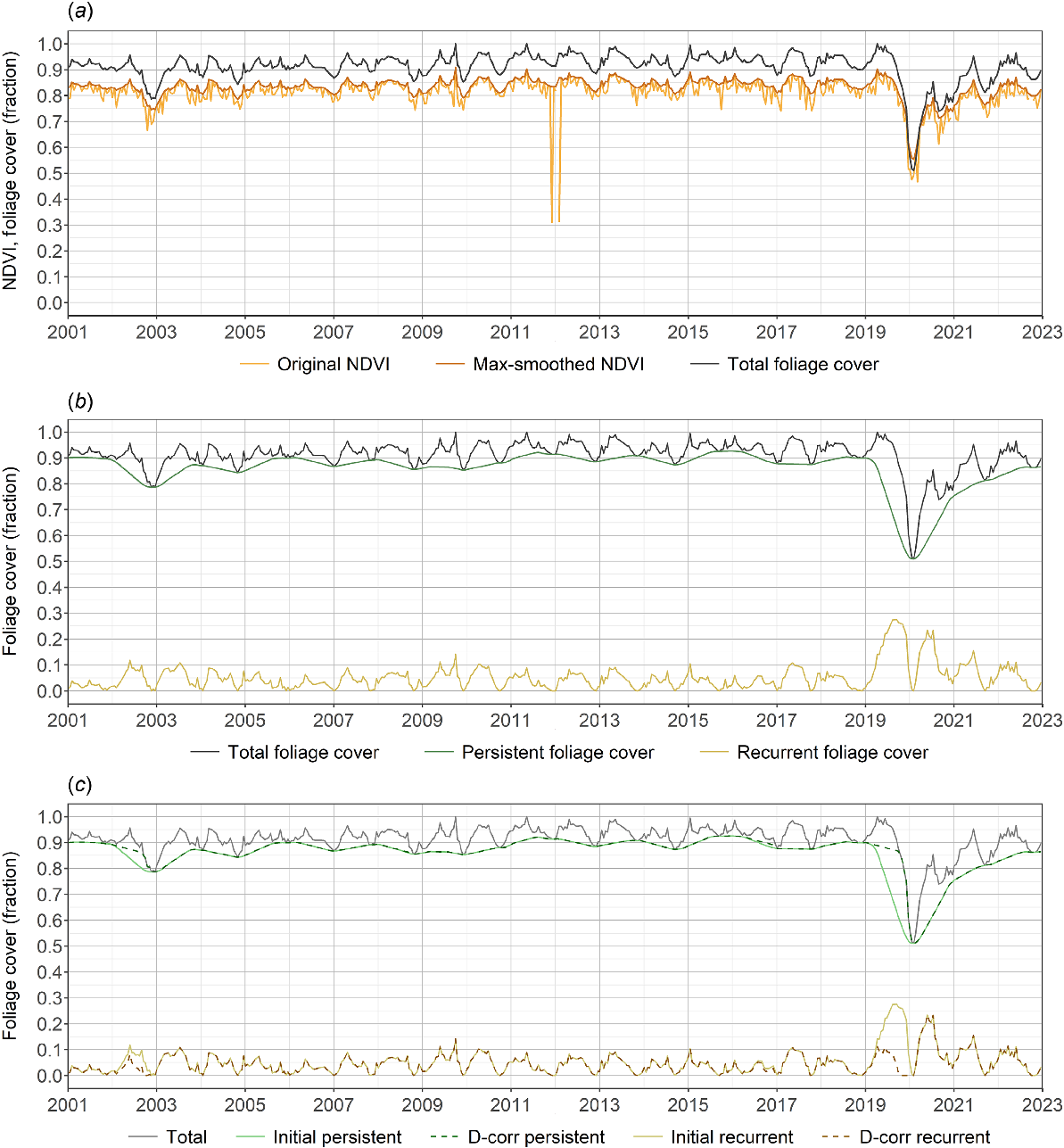
Here, V′ is the original NDVI, and i is the current time-step (which varies between 3 and m − 2). This smoothing is repeated such that the resulting NDVI is twice-smoothed. The degree of smoothing applied represents a balance between removing false drop-outs and data gaps on the one hand, and over-smoothing potentially validly low data on the other. Applying the maximum smoothing twice is seen as a reasonable compromise between these. An example of the effect of the maximum-smoothing algorithm is shown in Fig. 1a.
Examples of the stages in the calculation of total, persistent and recurrent foliage cover from NDVI. Data are from a wet sclerophyll forest site (Eucalyptus overstorey and shrub/fern understorey) in coastal NSW (150.00, −35.64). This site was burned in the 2019–2020 summer. (a) Original NDVI, maximum-smoothed NDVI and total foliage cover. (b) Persistent and recurrent foliage cover before the disturbance correction step. (c) The effect of the disturbance correction step (‘Initial’ denotes the time-series before correction, and ‘D-corr’ denotes those after correction).
Total foliage cover
Total foliage cover (F) is the fraction of ground covered by green foliage and can be estimated as a linear function of NDVI (Asrar et al. 1984; Carlson and Ripley 1997).
In this, Vmin is the minimum NDVI threshold (which represents the NDVI of bare ground for a given location), and Vmax is the maximum NDVI threshold (which represents the NDVI of complete, dense canopies).
The maximum NDVI threshold can be determined by examining the NDVI of locations known to have complete (100%) foliage cover. The full V time-series was examined at four undisturbed rainforest sites (ranging in latitude from −17.6° to −43.1°). The 90th percentile V was identified from the 2001 to 2018 time-series (intentionally excluding the 2019–2020 fires) at each of these four sites. The average of these values was 0.89 (with this differing across the four sites by 0.01) and Vmax was set to this value.
Unlike the maximum NDVI, the minimum NDVI threshold is known to vary substantially, predominantly with background soil type (Huete 1988; Qi et al. 1994; Yoshioka et al. 2000). Indeed, Montandon and Small (2008) showed that the NDVI of bare soil can vary between 0.05 and 0.40 (with the mean of a global soil database being 0.20). As the sensitivity of total cover to minimum NDVI is highest when foliage cover is low, accurate parameterisation of minimum NDVI is critical to retrieving accurate estimates of F across much of Australia. Parameterising this threshold is a significant challenge when soil characteristics are not accurately known a priori. In highly simplified approaches (Berry and Roderick 2002; Donohue et al. 2014), the threshold is treated as a constant; however, this results in systematic over- and under-estimation of cover in sparsely vegetated regions. In croplands, where it is reasonably certain that bare-ground conditions exist at least once during the MODIS record, Donohue et al. (2018) set this threshold to the lowest NDVI observed in the MODIS record. Where such a bare-ground assumption is not valid, an alternative approach for inferring soil NDVI is required.
The alternative approach used here partitions Australia into an ‘arid’ zone of low rainfall and low woody foliage cover, where it is reasonable to set the minimum threshold to the minimum-observed NDVI. The reciprocal ‘woody’ zone is where rainfall and woody foliage cover is higher and where the threshold needs to be inferred rather than observed (Fig. 2). A long-term mean V value of 0.25 is used to define these zones. This average value generally matches the drier limit of forests, savannas and temperate woodlands (DAWE 2020); it approximately corresponds to average rainfall isolines of 250 mm year−1 across the south of Australia and 450 mm year−1 across the north (Jones et al. 2009).
The minimum NDVI used to calculate total foliage cover. The arid and woody zones established for the calculation of minimum NDVI are shown as coloured or black areas respectively. The woody zone is where long-term average NDVI is greater than 0.25, and in this zone the minimum was inferred to be 0.2.
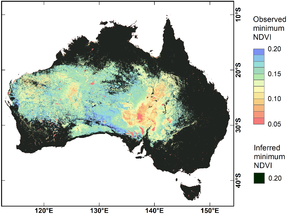
The minimum observed value from the full 2001–2022 V record is identified for all locations within the arid zone (Fig. 2). After setting a floor of 0.05 (as per Montandon and Small 2008), these minimum values are used to represent Vmin within this zone. Here, 0.05 corresponds to water bodies (largely intermittent) and salt pans, 0.1 corresponds to red–yellow siliceous sands, and values nearing 0.2 correspond to limestone and calcareous loam soils (CSIRO and National Resource Information Centre 1991). Outside this arid zone, in the woody zone, Vmin values are set to a static 0.20. This value was chosen because it is close to highest observed values within the arid zone (of 0.191) and because it is the stated average soil NDVI value in Montandon and Small’s (2008) global soils NDVI database. Note that, because the sensitivity of F to Vmin decreases as the total NDVI increases, the accuracy of Vmin is less important in the woody zone than in the arid zone. In summary, Vmin was calculated as follows.
Here, is long-term mean V, and V0 is the observed historical minimum V.
Persistent and recurrent foliage cover
Assuming that foliage cover of trees has low seasonal variability and that of grasses has high seasonal variability, the contribution of each vegetation type to total foliage cover can be approximated by separating the slow-changing and fast-changing (annual) components of the total cover time-series (Berry and Roderick 2002; Lu et al. 2003; Donohue et al. 2009). Persistent cover is the cover from vegetation that has perennial foliage. In Australia, where native deciduous trees and shrubs are almost absent, this generally equates to the foliage of woody plants (although this may include some sedges, rushes and ferns). Conversely, recurrent cover is the foliage cover from vegetation with annual foliage (which includes both perennial and annual grasses, plus forbs and other annuals). In this Australian context, recurrent foliage generally equates to grassy foliage. Although persistent and woody, and recurrent and grass, are approximately synonymous pairs, persistent and recurrent foliage cover will be used here to refer to generated cover estimates whereas woody and grass cover refer to actual or field-derived cover. Hence, the TSD model presented and modified here is called the persistent–recurrent splitting (PRS) algorithm.
The first step in the PRS algorithm is to fill any remaining gaps in the time-series with the long-term period-average total foliage cover. That is,
Here, is the period-average F of the 16-day period corresponding to i. A running minimum time-series is derived using a moving minimum window with a width of 17 periods (8.5 months), as follows:
where i ranges from 9 to m − 8. The running minimum is smoothed using a 15-period window (7.5 months), giving the estimate of persistent foliage cover (P), as follows:
Here i ranges from 8 to m − 7. Sometimes this results in persistent cover being higher than the original total cover, in which case persistent cover is set to total cover, that is
Recurrent foliage cover (R) is calculated as the difference between total and persistent cover, as follows:
An example of total, persistent and recurrent foliage cover is given in Fig. 1b.
A correction for major disturbances
The wet sclerophyll example in Fig. 1b shows the effect of using a moving minimum when there is a sudden and sustained decrease in total cover (such as after a fire or clearing). This causes a premature reduction of persistent cover (and an associated spike in recurrent cover) several months prior to the disturbance event. A correction for this is employed on the basis of the knowledge that, in the absence of a major disturbance, decreases in evergreen woody foliage cover are more gradual than sudden (Pook 1986). Thus, a maximum allowable rate of decrease in initial persistent cover was enforced at each time-step. This maximum rate of decrease was set at 0.002 (per 16 days). Whenever the persistent cover rate of decrease is more than this, it was reset to the previous time-step value minus 0.002 (with this reset value never being allowed to become greater that total cover), that is
The effect of this disturbance correction step can be seen in Fig. 1c. This is a particularly important adaptation of the underlying method for capturing the effects of land clearing and wildfires.
A correction for perennially green pastures
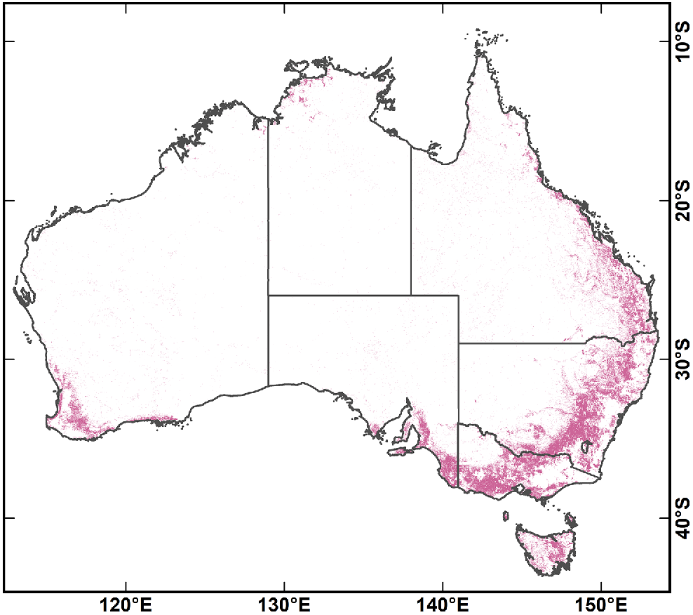
As so far described, the persistent–recurrent splitting algorithm is not effective for grasslands/pastures that remain green for most of the year, which is common in intensively managed, generally temperate pastures, and in irrigated pastures. When this happens, foliage cover is incorrectly interpreted as being persistent cover. With the correction, such situations are now identified using a mask of tree-free locations across the higher-rainfall regions of Australia. Wherever the treeless mask indicates a tree-free location, the full recurrent cover time-series is set to equal total cover, and persistent cover is set to zero.
This treeless mask is based on tree cover, vegetation type, and land use (Table 2) plus average total foliage cover (). Using GoogleEarth™ imagery for reference, the following rule set was developed:
If the land use of a location is ‘Irrigated pastures’ or ‘Irrigated cropping’, the location is treeless.
If a location is not in Tasmania (latitude <−39.3°), and is >0.4, and tree cover is <20%, and
-
the NVIS vegetation type is Tussock grassland or Other Grasslands, Herblands, Sedgelands and Rushlands or Cleared, or
-
the NSW vegetation type is Cleared,
then the location is treeless.
-
If a location is in Tasmania, and
-
is >0.5 but ≤0.7, and tree cover is <30%, or
-
is >0.7, and tree cover is <40%, or
-
the NVIS vegetation type is Other Grasslands, Herblands, Sedgelands and Rushlands,
then the location is treeless.
-
| Variable | Source | Pre-processing | |
|---|---|---|---|
| Tree cover (%) | Liao et al. (2020) | Compiled into a 2001–2021 average; resampled from 25- to 250-m spatial resolution. | |
| Native vegetation types (NVIS major vegetation groups) | DAWE (2020) | Resampled to 250-m spatial resolution. | |
| NSW vegetation formations and classes | Keith and Simpson (2012) | Resampled to 250-m spatial resolution; reprojected. | |
| Land use (catchment-scale land use of Australia) | ABARES (2021) | Resampled to 250-m spatial resolution. |
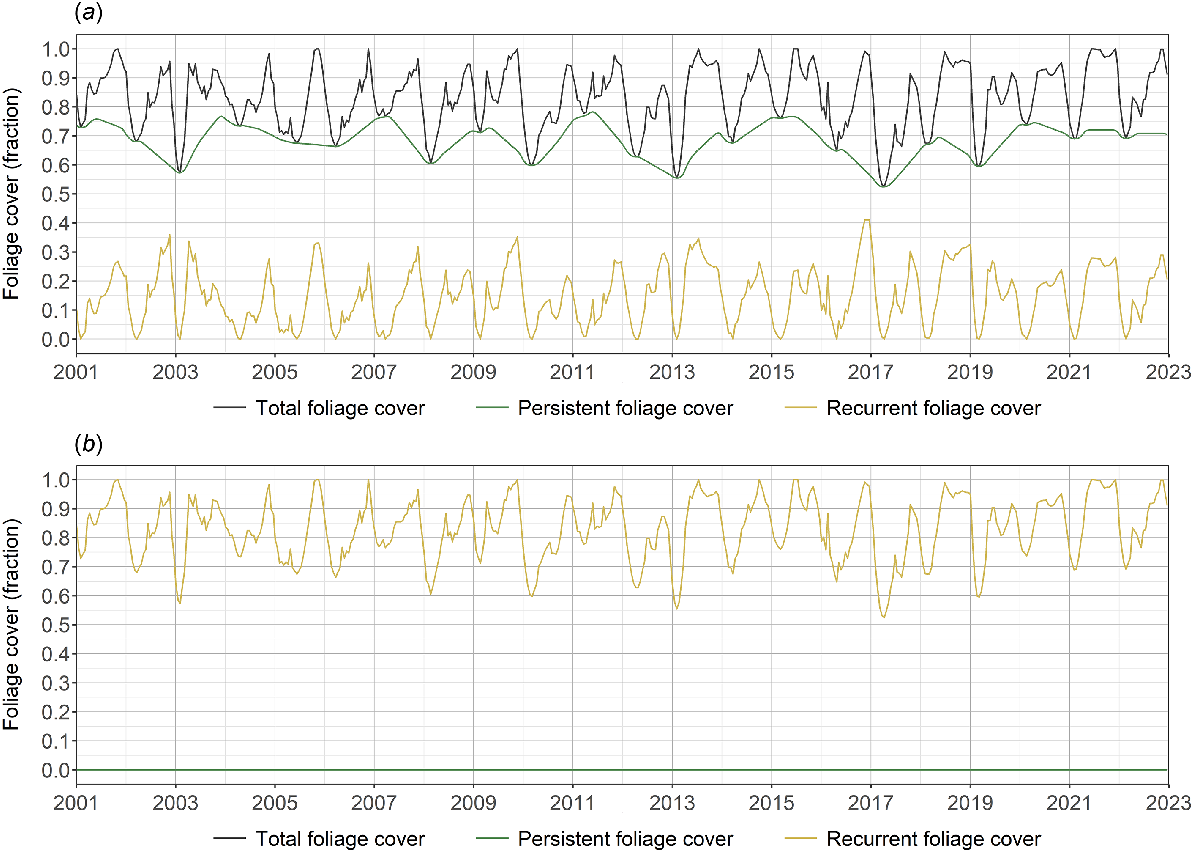
This mask is presented in Fig. 3, whereas Fig. 4 shows the effect of this perennially green pasture fix on cover estimates for a temperate pasture in southern Tasmania.
The treeless mask developed to identify perennially green pastures. Treeless areas are shown in pink.
Example of the correction for perennially green pastures. This site is a treeless, temperate pasture in southern Tasmania (146.934°, −43.153°). (a) The persistent–recurrent splitting algorithm estimates an average persistent foliage cover of 0.68. (b) After application of the perennial pasture correction, the average persistent cover has been reset to zero.
Validation
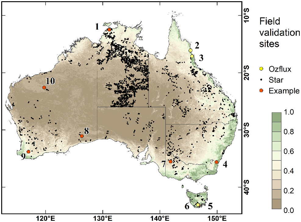
Field observations that describe total, woody and grass foliage cover fractions were obtained from the SLATS Stars Transect dataset (Department of Environment and Science 2022b). These data describe the percentage of ground covered by the green foliage from woody plants, measured at two heights (below 2 m and above 2 m), as well as the fraction of ground covered by live grass foliage (Muir et al. 2011). After removing some sites for quality reasons (see below), and after averaging multiple site values when sites shared grid cells, there were 4214 sets of observations from 3559 sites. The distribution of these sites is shown in Fig. 5. At each site, three intersecting, 100-m transects were laid out in a star pattern, and cover observations were taken at 1-m intervals along each. The values reported at each SLATS site are averages of all the transect point measurements. The dates of the field observations were aligned with their corresponding MODIS periods.
Locations of the field-derived foliage cover observations used to validate the total, persistent and recurrent foliage cover product. There are 3563 SLATS Star sites and three Ozflux sites. Labels for the Ozflux and ‘Example’ sites are: 1, savanna woodland; 2, Cape Tribulation; 3, Robson Creek; 4, temperate rainforest; 5, Eucalyptus tall open forest; 6, Warra; 7, Eucalyptus mallee; 8, Acacia woodland; 9, winter cereal cropping; and 10, hummock grassland. The Example sites are the locations for which time-series data are shown in Fig. 8.
It is difficult to know with the site-averaged SLATS data how each of the vegetation layers overlap and, therefore, how much cover of one layer may have been occluded by the one above (when viewed from above the canopy). Using an approach similar to that of Guerschman et al. (2015; Eqn 6), and by assuming that the spatial arrangement of the foliage of all layers is random, the occluding effect of overhead foliage can be incorporated into estimates of total woody foliage cover (FW), as follows:
Here, Fo and Fm are the over 2 m and under 2 m woody foliage cover respectively. Similarly, the occluding effect of the overhead woody cover on the grass cover can be approximated by rescaling the observed grass cover (Fg) in proportion to FW, as follows:
Here, FG is the rescaled site-average grass cover value. Observed total foliage cover is then calculated as the sum of FW and FG.
Observations of foliage cover taken from below the canopy have a similar but opposite occlusion effect in that upward-looking foliage observations can be occluded by branches. This effect can also be approximated using the same logic as used for correcting top-down occlusion (see Armston et al. 2009). However, we tested the difference in estimates of FW when bottom-up occlusion is and is not accounted for, and the difference was negligible (<0.01 for the SLATS data), and so here we ignore this effect.
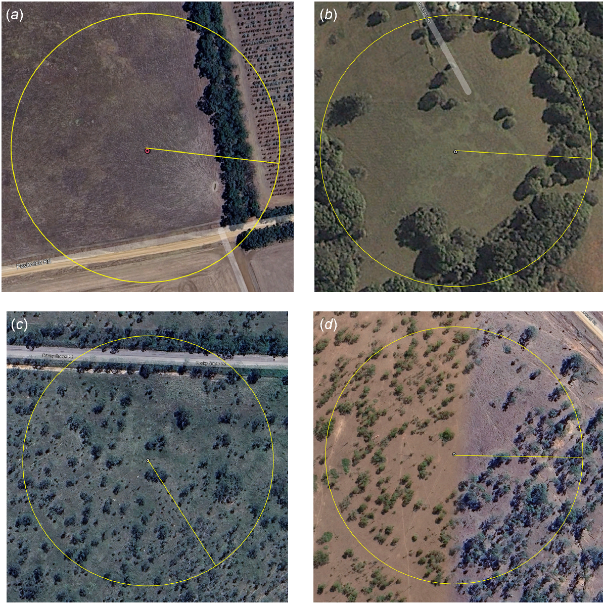
Using GoogleEarth™ imagery from the year closest to the date of the field observations, we checked each SLATS site described as dense grasslands (that is, FW = 0 and FG ≥ 0.8) for the presence of trees/shrubs. Of 33 dense grasslands sites, nine were found to have a substantial number of trees within 250 m of the central location of the site, and were removed from analyses. Some of these nine sites had trees only towards the periphery of the circle (Fig. 6a, b), which reflects a genuine scale-mismatch in the validation approach. The remainder of the nine sites had trees scattered throughout the field plot (Fig. 6c, d), even though the observed tree cover was zero. A similar examination of a sample of the 139 SLATS grassland sites (FW = 0 and 0.3 < FG < 0.8) showed far fewer sites having this problem.
Examples of field sites recorded as having zero woody cover. Each site is a dense (and treeless) grassland according to the field-recorded cover values. However, each has trees surrounding or within the field plot according to high-resolution satellite imagery. Yellow circles show a 250-m-diameter circle around the centre of each plot. (a, b) Sites with trees only around the periphery of the circle, which have been correctly assessed as being treeless at the 100-m field-plot scale but which are tree–grass mixtures at the 250-m grid-cell scale. (c, d) Sites with scattered trees across the whole site, meaning that the field data incorrectly describe these sites as having no tree foliage cover. Imagery derived from Google Earth© 2024 – Landsat/Copernicus/Maxar.
The locations of the SLATS Star data points, shown in Fig. 5, are heavily biased towards the drier and sparsely wooded regions of Australia. To provide extra observations at the opposite end of the cover spectrum, several rainforest and wet forest sites were included in the validation. Six total foliage cover values were included from three Ozflux sites (Fig. 5), namely, Warra Tall Eucalypt (Wardlaw 2023); Robson Creek Rainforest (Bradford and Ford 2022); and Daintree Rainforest, Cape Tribulation (Liddell and Laurance 2024). The reported foliage cover values at each site had been calculated from LAI, which itself was derived from fisheye lens photographs (see Karan 2015). In these few Ozflux sites it was assumed that woody and total foliage cover were the same thing.
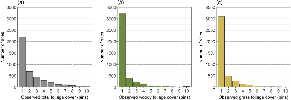
The distribution of the field sites is heavily biased to the arid rangelands of Australia and to the Northern Territory in particular (Fig. 5). The majority of sites (50%) come from locations with extremely low total foliage cover (<0.1), whereas only 10% of sites have total cover >0.5 (Fig. 7). The representation of woody and grassy cover is even more extreme, with 74% and 71% of sites having woody and grass cover of <0.1.
Number of field observations across the full range of cover values. Observations are summarised by 0.1-wide bins of observed foliage cover, starting at 0.0 (so, for example, Bin 1 extends from 0.0 to 0.1, and bin 10 spans from 0.9 to 1.0) for (a) total cover, (b) woody cover and (c) grass cover.
Results
Total, persistent and recurrent foliage cover through time
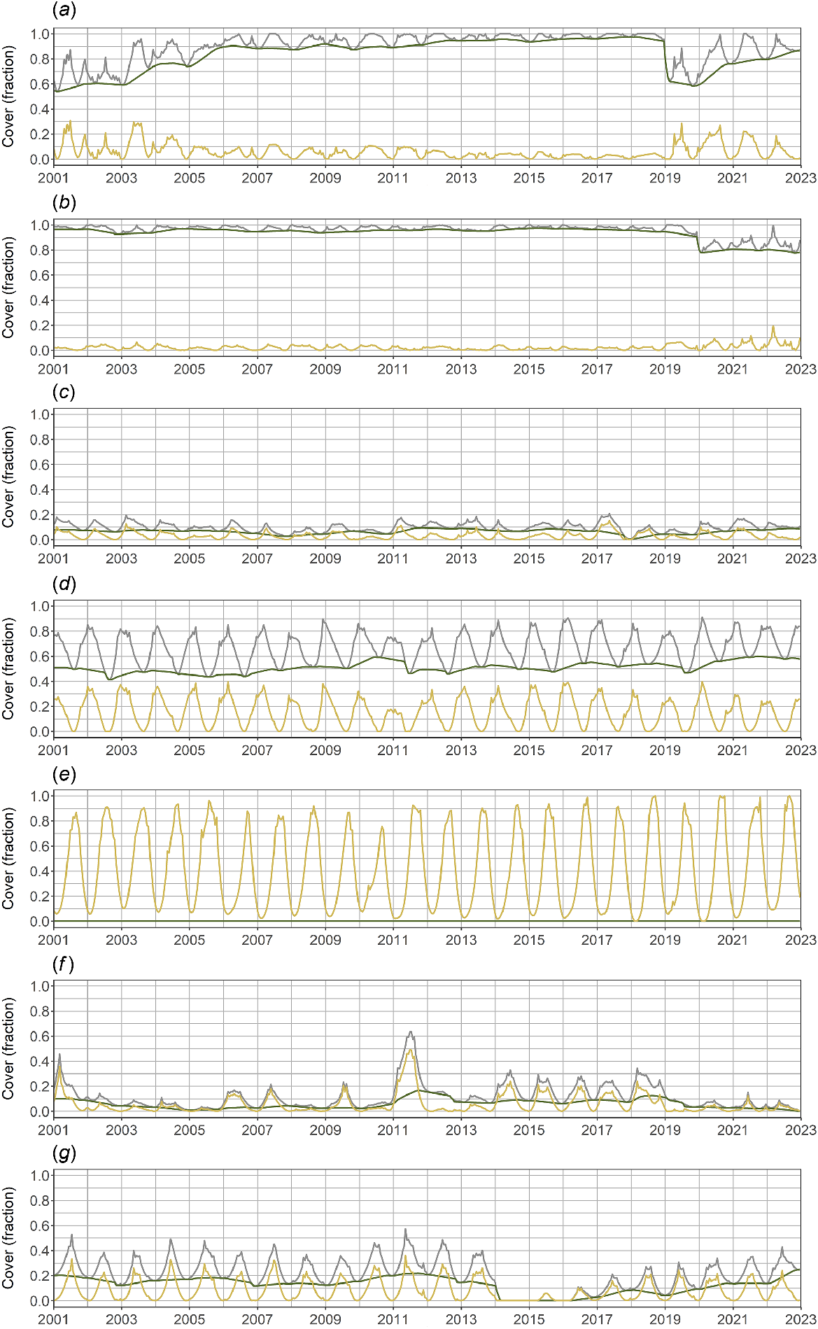
The temporal dynamics in the total, persistent and recurrent foliage cover estimates for seven example sites are shown in Fig. 8. The location in Fig. 8a is a Eucalyptus tall open forest with a rainfall of 1350 mm year−1. This site was logged in 2000 and then burnt in early 2019. This example shows the response of persistent (woody) and recurrent (grass) cover following major disturbances. The location in Fig. 8b is a temperate rainforest with a rainfall of 950 mm year−1. Here, there is effectively no recurrent cover (or none seen from above) and a constantly closed forest canopy, except after a fire in late 2019. The location in Fig. 8c is a semiarid hummock (Triodia spp.) grassland with a rainfall of 360 mm year−1. Here, there are sparse shrubs among the hummocks, which gives rise to low persistent cover. The location in Fig. 8d is a savanna woodland with a rainfall of 1681 mm year−1. The monsoon-driven grass dynamics are evident (peaking in the austral summer) as is the cover of the open woodland overstorey. The location in Fig. 8e is a winter cereal crop with a rainfall of 490 mm year−1. Without the perennially green grassland correction, the persistent cover at this site would incorrectly be estimated at ~0.1. The location in Fig. 8f is from an arid Acacia woodland with a rainfall of 210 mm year−1. The responses of the Acacia tree cover and the underlying grass cover to a very wet year in 2011, and then the ongoing effect of a very dry year in 2019, are evident. The location in Fig. 8g is a semiarid Eucalyptus mallee woodland with a rainfall of 310 mm year−1. A fire in 2014 reduced cover to zero, and low rainfall in the following 2 years resulted in a slow post-fire recovery of cover.
Total, persistent and recurrent fractional cover time-series from a selection of sites across Australia. The three cover types are represented by black, green and brown lines respectively. (a) Eucalyptus tall open forest in southern Tasmania (146.752°, −43.114°); (b) temperate rainforest on the southern coast of NSW (149.898°, −35.627°); (c) hummock grassland in the Pilbara, Western Australia (119.772°, −22.588°); (d) savanna woodland in the north of the Northern Territory (131.152°, −12.494°); (e) winter cereal cropping in south-west Western Australia (117.024°, −33.809°); (f) Acacia woodland on the Nullarbor Plain, Western Australia (126.366°, −31.08°), and (g) Eucalyptus mallee woodland in western Victoria (141.882°, −35.529°). The locations of these sites are shown in Fig. 5 as ‘Example’ sites.
Total, persistent and recurrent foliage cover across Australia
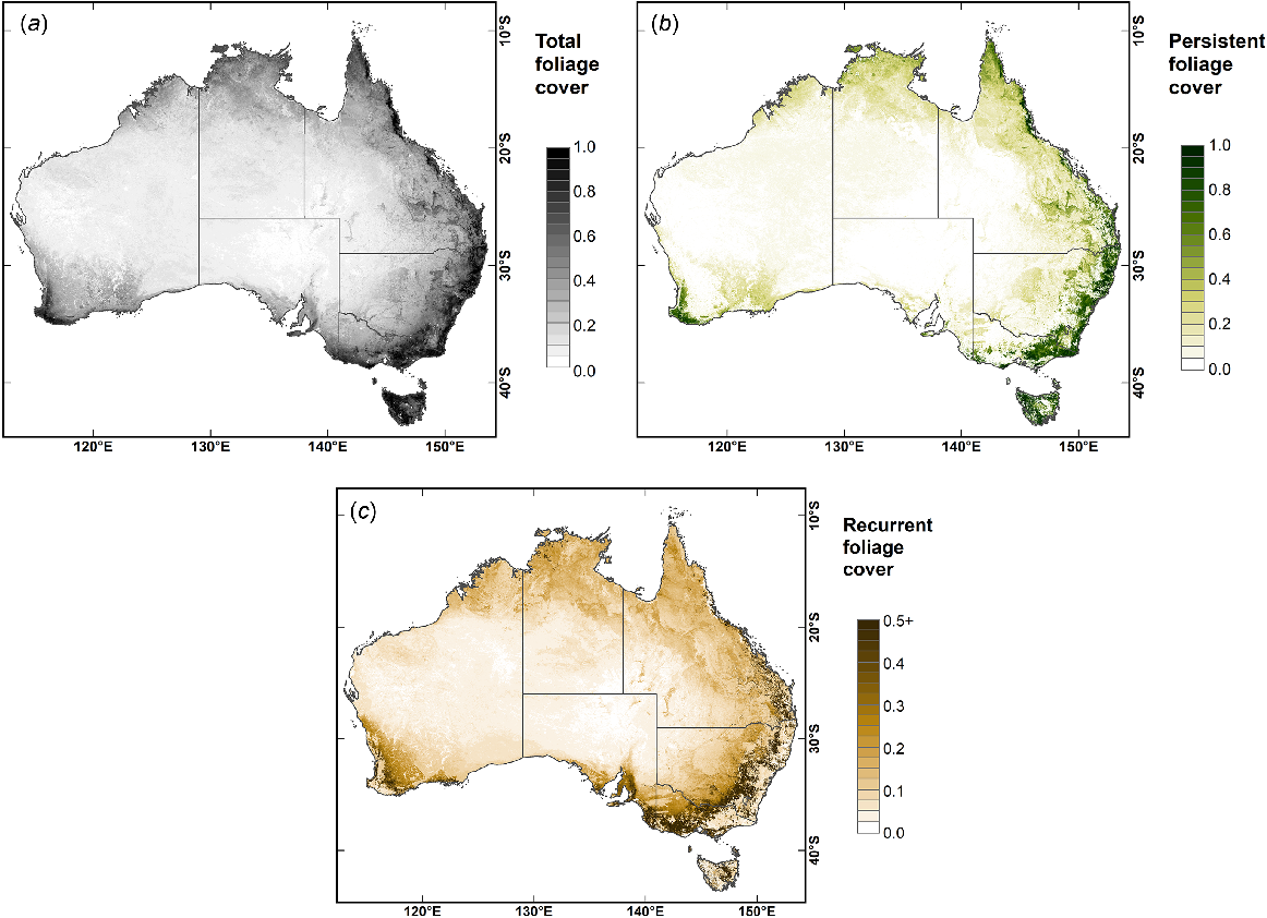
The spatial patterns of average foliage cover across Australia are shown in Fig. 9. These reflect the known distributions of general ecosystem productivity, which, in Australia, follow patterns of total rainfall (Specht 1972). The highest persistent cover (>0.8) aligns with the distribution of forests, and moderate persistent cover (approximately 0.5–0.8) aligns with woodlands and shrublands (DAWE 2020). The highest average recurrent cover values occur in the high-rainfall regions of the intensive agriculture zone (which have largely been cleared). Note that the average foliage cover of pure grasslands peaks at ~0.5. The arid centre of Australia has low cover of either vegetation type.
Validation of foliage cover estimates
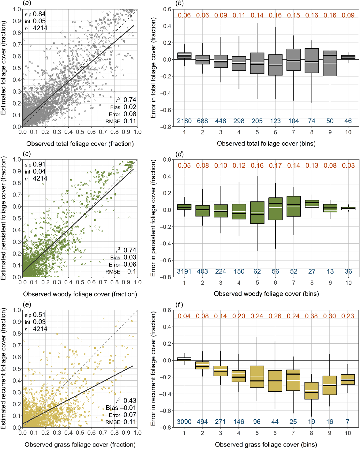
The comparison of the three foliage cover estimates with field-observed cover is shown in Fig. 10. Here, errors are reported as the bias (the mean error, ME) and the ‘error’ (which is the mean absolute error, MAE). Only in Fig. 10 is the root mean square error (RMSE) reported to facilitate comparisons with the errors reported for equivalent data products in Table 1. Fig. 10 shows that overall errors (and biases) are 0.08 (0.02), 0.06 (0.03) and 0.07 (−0.01) for total, persistent and recurrent cover respectively. Both the total and persistent estimates represent linear and reasonably unbiased predictions (overall) of the observed values, whereas the recurrent estimates generally under-estimate the observed values. Most observations come from sparsely vegetated environments (where cover is <0.1; Fig. 7), which biases statistics towards the errors obtained in such environments. Hence, more useful insights are gained if errors are examined across the range of cover values. To this end, the cover fractions from 0 to 1 are divided into 10 equally sized bins (Fig. 10b, d, f). Outside of sparsely vegetated environments, the errors (and bias) for total, persistent and recurrent cover are 0.12 (−0.03), 0.11 (0) and 0.23 (−0.21) respectively (corresponding to the average error across Bins 2–10; Fig. 10). Estimates of persistent cover slightly, but systematically, under-estimate woody cover between cover of 0.1 and 0.5 and then slightly over-estimate cover at higher values. Overall, however, persistent cover is the most accurately predicted of the three cover types. In contrast, recurrent cover is the most poorly estimated cover type, consistently under-estimating grass cover at sites with grass cover greater than 0.1, with maximum errors (up to 0.38) for the denser grasslands.
Validation of total, persistent and recurrent foliage cover. Estimated (a) total, (c) persistent, and (e) recurrent values are compared against observed total, woody, and grass foliage cover, all respectively. The slope (slp) and intercept (int) of the linear fit are shown in each plot, along with the number of observations (n). (b, d, f) The errors summarised by 0.1-wide bins of observed foliage cover, starting at 0.0 (so, for example, bin 1 spans from 0.0 to <0.1, and bin 2 spans from 0.1 to <0.2; note that bin 10 spans from 0.9 to 1.0 inclusive). Boxes span the inter-quartile range of errors; tails show the range of the central 95% of error values. The thick black and white horizontal lines show the median and mean errors respectively. The error (MAE) for each bin is given by the orange text (on top) and the number of data points in each bin is given by the blue text (at the bottom).
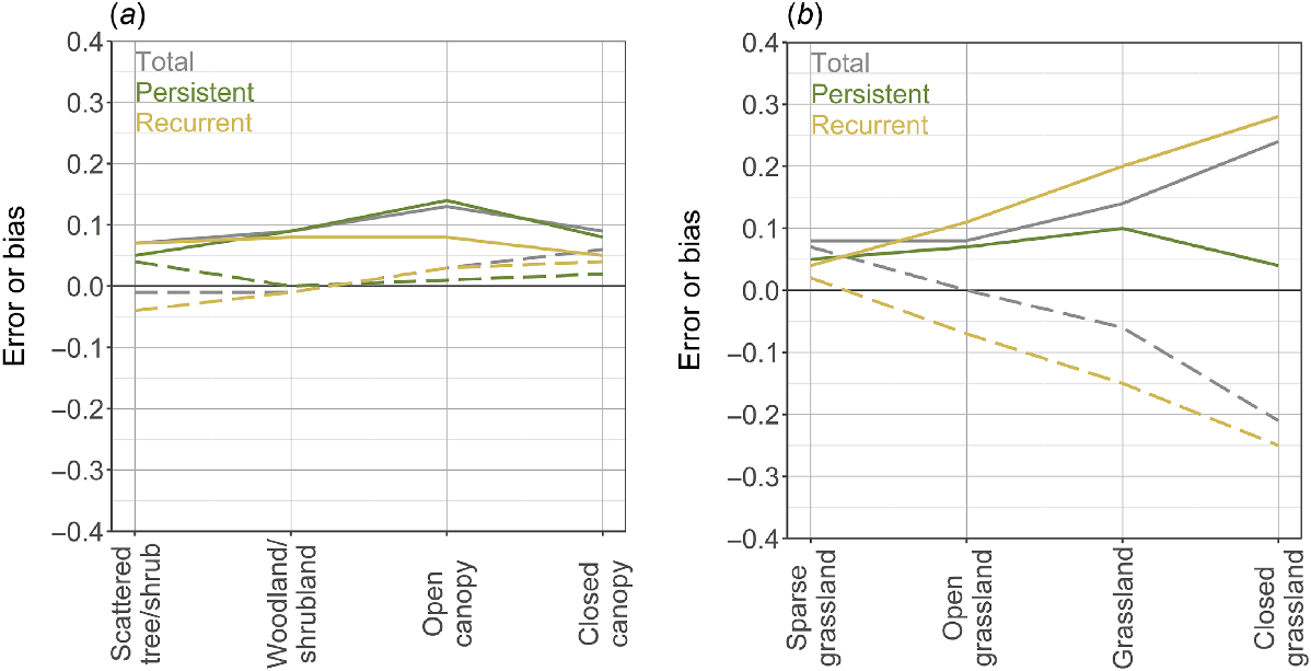
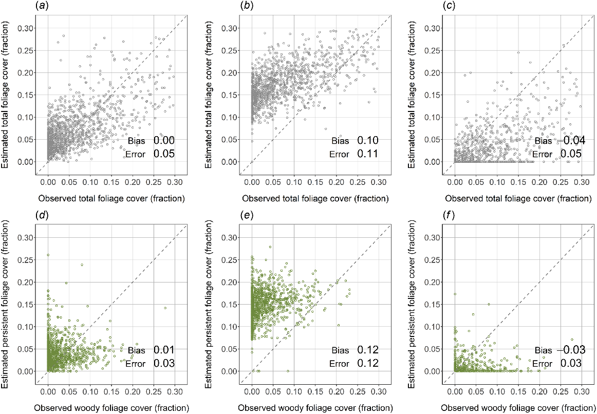
Further insights into the errors are obtained by separating results into vegetation structural classes (Table 3). These classes follow the structural definitions of Specht (1970), which are commonly used in Australia. Fig. 11 summarises the errors and biases for the wooded and grassland structural classes, while Fig. 12 presents the validation scatter plots, which give an indication of the spread of errors.
| Structural class | Description | |
|---|---|---|
| Wooded | ||
| Closed canopy | F W > 0.7, F G > 0.0 | |
| Open canopy | F W 0.3–0.7, F G > 0.0 | |
| Woodland/shrubland | F W 0.1–0.3, F G > 0.0 | |
| Scattered tree/shrub | F W 0.01–0.1, F G > 0.0 | |
| Grassland | ||
| Closed grassland | F G > 0.7, F W = 0.0 | |
| Grassland | F G 0.3–0.7, F W = 0.0 | |
| Open grassland | F G 0.1–0.3, F W = 0.0 | |
| Sparse grassland | F G 0.01–0.1, F W = 0.0 | |
| Unvegetated | F W = 0.0, F G = 0.0 | |
In Description, FW and FG stand for the observed woody foliage cover and observed grass foliage cover respectively. Note that woody cover does not discriminate between shrubs and trees, nor between understorey and overstorey woody foliage. For the woody structural types, sites with zero grass cover were excluded to minimise the biases originating from the large number of such sites.
Summary of the error and bias for wooded and grassland vegetation structural types. Results (a) for wooded structural classes and (b) for grassland classes. Classes are listed on the x-axis in order of increasing foliage cover. Solid lines show the error (MAE) and dashed lines show the bias (ME).
Comparison of estimated and observed woody and grass foliage cover for various vegetation structural types. In each graph, green represents persistent/woody cover and brown represents recurrent/grass cover. Linear best-fit lines are shown in colour.
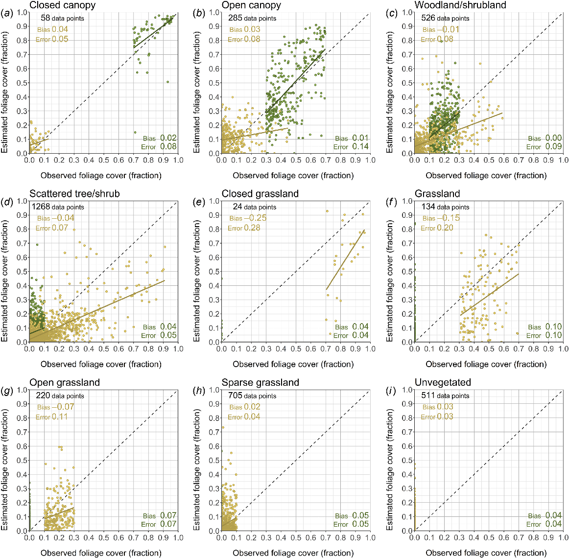
For wooded structural classes, errors in all three cover types are reasonably constant and low across the range of foliage densities. Errors range between 0.05 and 0.14, and are centred around 0.09 for total and persistent cover and around 0.07 for recurrent cover. Biases for all cover types are also small, ranging between −0.05 and 0.05. Overall, the total, woody and grass cover are predicted with reasonably high accuracy for these wooded structural classes. In contrast, predictions for grassland structural classes have errors and biases that scale with foliage density and become quite large. Errors are lowest for sparse grasslands and highest for dense grasslands, with total and recurrent cover having errors as large as 0.24 and 0.28 respectively. Persistent cover errors remain reasonably low. Biases for total and recurrent cover become increasingly negative as grass cover increases, meaning that these cover types are increasingly under-predicted as grassland density increases. Given that errors in recurrent cover mirror those in total cover, the inaccuracy is likely to originate from the calculation of total cover rather than in the PRS algorithm.
The approach used here to parameterise minimum NDVI (Vmin) allowed for a spatially varying minimum; it was calculated as the minimum observed NDVI within the arid zone (and set as a constant 0.2 elsewhere). Fig. 13 shows the effect this new approach has on the calculation of total and persistent cover in sparsely vegetated landscapes (which is where cover calculations are most sensitive to the accuracy of Vmin). The new approach is compared with two alternative parameterisations, one which sets Vmin as a constant 0.05 and the other as a constant of 0.20 (both of which have been used in previous versions of this PRS algorithm). The new parameterisation is appreciably more accurate that when setting Vmin to 0.05 and is of comparable accuracy to when Vmin is set 0.20, but now with no bias.
Demonstration of the effects of the minimum NDVI value on estimates of total and persistent foliage cover. These sites are from within the ‘arid’ zone that was used to calculate Vmin. (a–c) Total foliage cover calculated when Vmin is the minimum observed NDVI (the method described in this paper), or is set to 0.05 or 0.20 respectively. (d–f) The same, except for persistent foliage cover.
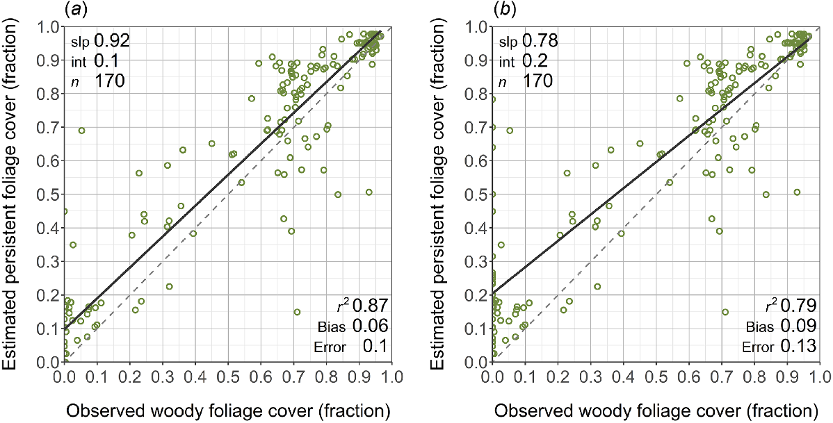
One improvement incorporated into the PRS algorithm is the perennial pastures correction, which aims to force the algorithm to recognise the cover from perennially green pastures as recurrent cover rather than persistent cover. Fig. 14 shows the effect of this correction on densely vegetated sites (woody cover >0.7). Although the differences between the two results are moderate, the perennial fix has improved results, causing a 0.03 reduction in both the error and bias.
The effect of the correction for perennially green pastures on estimates of persistent foliage cover. Here, only sites with observed total cover of >0.7 are shown. Here, persistent cover estimates are compared to observed woody cover observations when (a) the perennially green pastures correction is used, and when (b) the correction is not used.
Discussion
The two aims of this work are to enhance the performance of the overall method in three specific aspects (improve accuracy in arid environments, around major disturbances and in perennially green pastures), and to quantify the accuracy of the resulting foliage cover estimates. The new method of estimating Vmin has removed the overall bias in persistent cover estimates in arid environments, and the implementation of the perennial pasture fix within the PRS algorithm has reduced both error and bias. The effect of the fix for major disturbances in the PRS algorithm has not been quantitatively assessed because of a lack of suitable time-series cover observations during major disturbance events. However, intuitively, the fix has improved the realism of the cover estimates immediately prior to disturbances (see Fig. 1c). The second aim of this work was to quantify the accuracy of the total, persistent and recurrent estimates. Here, the estimates have been tested across the full range of cover values and vegetation structural classes, which is a level of detail not previously reported for an Australian cover product.
At the global level (all data pooled), the validation shows that the performance of this method is equivalent to that reported for similar Australian cover products (that is, RMSEs of ~0.10 for both total and persistent cover). According to the MAE, errors are closer to 0.08 and 0.06 for total and persistent cover (or, equivalently, accuracies of 92% and 94%). The global recurrent cover error is 0.07. However, because of the heavy bias of the field data towards very sparsely vegetated landscapes, these global statistics do not usefully capture performance. When assessed across the cover values and structural classes, persistent cover is the most consistently and accurately estimated cover type, with errors between 0.05 (for sparse woody/grass cover) and 0.14 (for dense woody/grass cover). Over woody vegetation classes, total and recurrent cover errors are similarly constant and low (ranges of 0.07–0.13 and 0.05–0.08 respectively). However, over grasslands, total and recurrent errors are larger and scale with grass foliage cover, with the higher errors occurring over dense grasslands (with large, negative biases). Evidently, this revised methodology works well over woody landscapes, even those with sparse tree cover, but it has systematic errors in estimating total and recurrent cover in treeless areas.
One possible source of this error is the highly dynamic nature of grass foliage cover. Matching day-specific field dates with 16-day satellite composite dates potentially introduces temporal mismatches of up to 15 days. However, for this to have caused the systematic underestimation of cover, it would require the mismatch to be systematically early during green-up and/or late during brown-down. Investigation of timing mismatches did not indicate that this is likely.
Another possible source of error is in the field measurements themselves. The observations reported cover from three heights, namely, ground foliage cover, woody foliage cover under 2 m, and woody foliage over 2 m, which makes it a remarkably rich dataset. However, there is no explanation provided on how each of these layers overlap. From above the canopy, as viewed from a satellite, woody foliage cover will occlude any grass cover directly below and so, if the reported grass cover values are taken as-is, they will represent some degree of overestimation. The rescaling of the observed grass cover in proportion to the woody overhead foliage cover (Eqn 11) attempted to limit this possibility.
The systematic underestimation of total and grass foliage cover over grasslands indicates a methodological shortcoming. Given that the error is an underestimation, this could mean that the method for rescaling of NDVI to cover for grasslands needs different parameterisation than that used for woody vegetation. Setting a lower maximum NDVI threshold for grasslands than for woody landscapes would increase both total and grass cover estimates, as might raising the minimum NDVI threshold. But such changes should be made only if underpinned by sound biophysical reasoning.
Another potential focus for improving this method is how the minimum NDVI threshold is identified, which is aimed at capturing the background soil NDVI. The current method used can be applied only to very sparsely vegetated landscapes (which, conveniently, are the locations where it is most important to accurately estimate this threshold). However, a more robust method would be to model background NDVI by using independent soil information. For example, it can be reasonably assumed that the spectral properties of soils of different types generally remain invariant across the country (wetting and surface-water ponding notwithstanding). As such, it may be possible to infer estimates of Vmin by using statistical or machine-learning approaches trained on soil texture data and historical V obtained for parts of the country that can be effectively categorised as bare ground. This would exploit newly developed gridded representations of soils attributes (e.g. Dobarco et al. 2024) to enable spatially varying Vmin for locations in the current algorithm set to 0.2, and would lessen the need for a multi-decade satellite imagery from which the lowest NDVI must be identified.
Although this method has been applied to MODIS imagery, it is not restricted to such imagery. Notionally it can be readily translated to any alternative moderate resolution imagery with similar temporal time-steps (such as VIIRS), although the alternate imagery would require a similarly long record for identifying the minimum NDVI threshold (or an alternative method for identifying it). Applying this method to higher-resolution imagery, such as Landsat or Sentinel-2, would require modifications to account for any differences in the temporal time-step (such imagery currently needs to be composited to quarterly time-steps or longer to minimise cloud-induced no-data gaps typical of these sources).
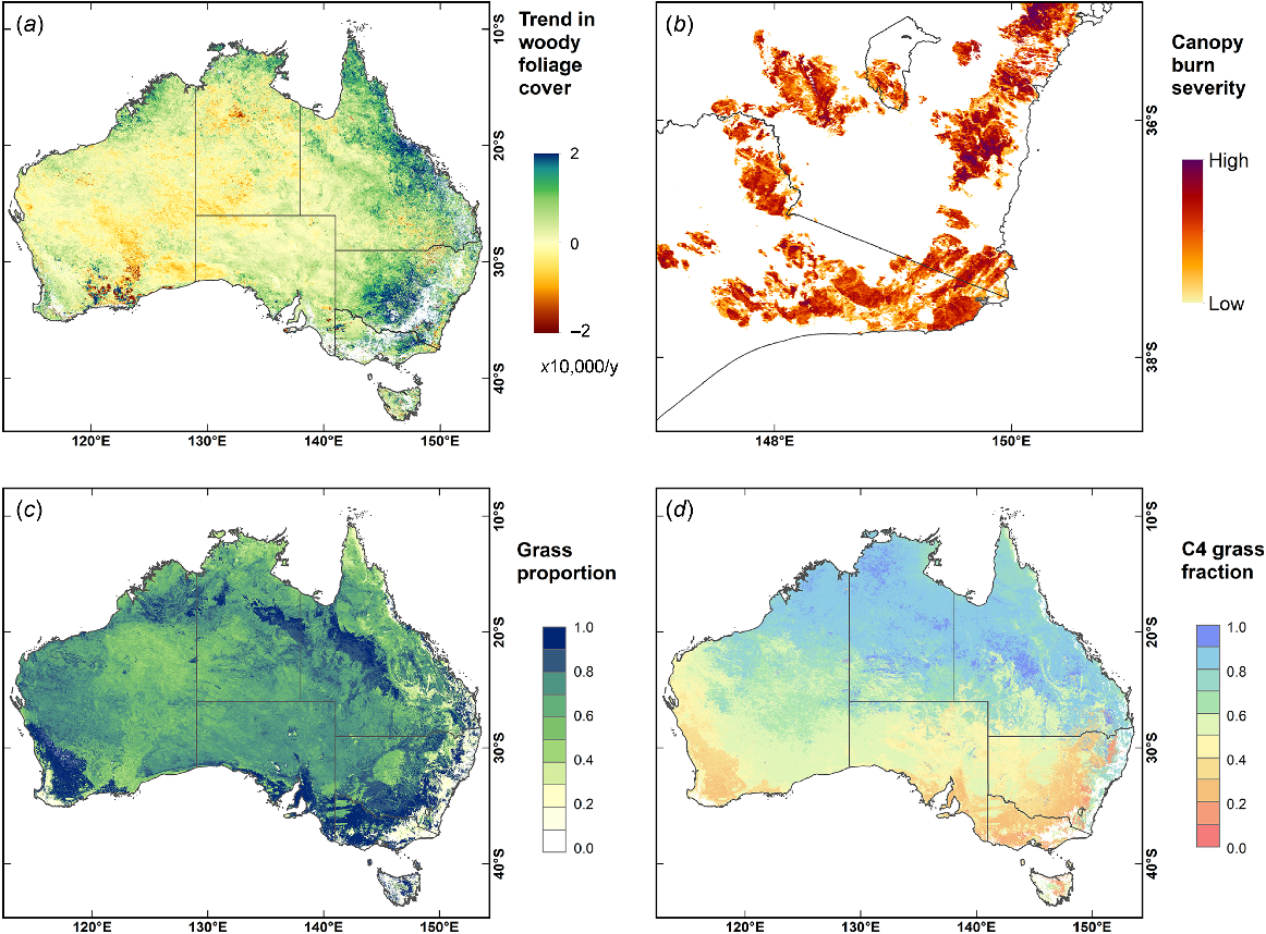
In terms of overall accuracy, this new fractional cover product is equivalent to existing Australian products for total and woody cover. What makes it unique is that woody foliage cover is estimated at a near-fortnightly frequency (other products report woody cover either quarterly or annually). However, more significant is that this is the only product that provides estimates of grass cover outside of pure grasslands and pastures (where total foliage cover equates to grass cover). This method generates grass cover estimates in mixed woody–grassy landscapes, such as in tropical savannas, shrubby grasslands and grassy woodlands. The value of temporally dense woody and grass foliage cover data is that they reveal subannual and even subseasonal temporal dynamics. The power of this can be demonstrated through a selection of cover-derived vegetation products (Fig. 15). Long-term changes in foliage cover can be identified separately for woody and grassy vegetation (Fig. 15a), which is particularly useful for tracking the impact of land management changes because these have historically promoted grass cover over woody cover (Berry and Roderick 2006). The severity to which forest canopies are burned by wildfires can be assessed (Fig. 15b) by comparing the woody foliage cover immediately preceding a fire to that in the month or two following the fire. The distribution of pure grasslands, mixed grasslands, and grassy woodlands can be found using the grass proportion (Fig. 15c). This shows different information than grass foliage cover alone, as pure grasslands need not have high foliage densities. Finally, the distribution of C4 grasses can be estimated (Fig. 15d) by examining the within-year timing of peak grass foliage cover, because C4 species peak in late summer/early autumn, whereas C3 grass species peak in late spring/early summer (Hattersley 1983; Johnston 1996).
Examples of products that can be uniquely derived from temporally dense woody and grass foliage cover data. (a) The linear trend in woody foliage cover between 2001 and 2023. (b) The canopy burn severity of the 2019–2020 ‘Black Summer’ fires, derived from time-series woody foliage cover data. (c) The grass proportion, which is the ratio of grass to total foliage cover. Here, a value of one represents pure grasslands and a value of 0.5 indicates an even mix of woody and grass cover. (d) The estimated fraction of C4 grasses (Donohue 2023).
Conclusions
Of the various methods used to estimate foliage cover from satellite imagery, only time-series decomposition-based methods can currently generate temporally dense estimates of both woody and grass cover. The work presented here represents the latest iteration of a woody–grass foliage cover method that is built around the persistent–recurrent splitting algorithm, which itself has been under development for the past two decades. This iteration focusses on improving accuracy in arid environments, around major disturbances and in perennially green pastures. This work represents the first time this method has been comprehensively validated. Overall performance was found to be equivalent to that of alternative methods that generate annual or seasonal total and woody cover. Cover estimates were also assessed across a range of cover values and vegetation structural classes, revealing a distinct difference in performance between woody and grassland vegetation. Estimates of total, woody and grass fractional cover have consistently low errors and are unbiased over woody vegetation, with errors centering around 0.08 and ranging between 0.05 and 0.14 (or, conversely, with accuracies of ~92% and ranging between 86% and 95%). However, by contrast, accuracy diminishes over grasslands as actual foliage cover increases, with errors in total and grass cover increasing up to 0.23 and 0.34 respectively, and with estimates becoming increasingly underpredicted. The value of this method lies in its ability to generate temporally dense foliage cover data that can be used to monitor vegetation dynamics and change, most particularly across Australia’s mixed tree-grass landscapes.
Data availability
The foliage cover data described here are freely available and can be downloaded from http://hdl.handle.net/102.100.100/658533.
Declaration of funding
The Australian Climate Service contributed funding for this research through CSIRO’s National Bushfire Intelligence Capability, which is also supported by the National Emergency Management Agency.
References
ABARES (2021) Catchment scale land use of Australia – update December 2020. Australian Bureau of Agricultural and Resource Economics and Sciences. Available at https://doi.org/10.25814/aqjw-rq15
Armston JD, Denham RJ, Danaher TJ, Scarth PF, Moffiet TN (2009) Prediction and validation of foliage projective cover from Landsat-5 TM and Landsat-7 ETM+ imagery. Journal of Applied Remote Sensing 3(1), 033540.
| Crossref | Google Scholar |
Asrar G, Fuchs M, Kanemasu ET, Hatfield JL (1984) Estimating absorbed photosynthetic radiation and leaf-area index from spectral reflectance in wheat. Agronomy Journal 76(2), 300-306.
| Crossref | Google Scholar |
Berry SL, Roderick ML (2002) Estimating mixtures of leaf functional types using continental-scale satellite and climatic data. Global Ecology and Biogeography 11(1), 23-39.
| Crossref | Google Scholar |
Berry SL, Roderick ML (2006) Changing Australian vegetation from 1788 to 1988: effects of CO2 and land-use change. Australian Journal of Botany 54(4), 325-338.
| Crossref | Google Scholar |
Bowman DMJS, Prior LD (2005) Why do evergreen trees dominate the Australian seasonal tropics? Australian Journal of Botany 53(5), 379-399.
| Crossref | Google Scholar |
Bradford M, Ford A (2022) Robson creek rainforest vegetation structure data, 2014. Version 1.0. Terrestrial Ecosystem Research Network. Available at https://doi.org/10.25901/7brp-f114
Brockerhoff EG, Barbaro L, Castagneyrol B, Forrester DI, Gardiner B, González-Olabarria JR, Lyver P, Meurisse N, Oxbrough A, Taki H, Thompson ID, van der Plas F, Jactel H (2017) Forest biodiversity, ecosystem functioning and the provision of ecosystem services. Biodiversity and Conservation 26(13), 3005-3035.
| Crossref | Google Scholar |
Carlson TN, Ripley DA (1997) On the relation between NDVI, fractional vegetation cover, and leaf area index. Remote Sensing of Environment 62(3), 241-252.
| Crossref | Google Scholar |
Collett L (2024) Foliage projective cover – Sentinel-2, DES algorithm, QLD coverage. Version 1.0. Department of Environment and Science, Queensland Government. Available at https://portal.tern.org.au/metadata/TERN/c65ad708-e270-431a-bb5b-13f1a4ec13db
Cranko Page J, Abramowitz G, De Kauwe MG, Pitman AJ (2024) Are plant functional types fit for purpose? Geophysical Research Letters 51(1), e2023GL104962.
| Crossref | Google Scholar |
CSIRO and National Resource Information Centre (1991) Atlas of Australian soils (digital), version 3. CSIRO. Available at 10.25919/5f1632a855c17
Department of Environment and Science (2021) Foliage projective cover – Landsat, DES algorithm, QLD coverage. Version 1.0. Department of Environment and Science, Queensland Government. Available at https://portal.tern.org.au/metadata/TERN/508f322a-a9fd-459f-9122-df52e2b6579e
Department of Environment and Science (2022a) Seasonal persistent green – Landsat, JRSRP algorithm version 3.0, Australia coverage. Department of Environment and Science, Queensland Government. Available at https://portal.tern.org.au/metadata/TERN/dd359b61-3ce2-4cd5-bc63-d54d2d0e2509
Department of Environment and Science (2022b) SLATS star transects – Australian field sites. Version 1.0. Department of Environment and Science, Queensland Government. Available at https://portal.tern.org.au/metadata/TERN/24a40c29-0d7c-4fe8-bdde-9c4ea495bfb8
Dobarco RM, Wadoux A, Malone B, Minasny B, McBratney A, Searle R (2024) Soil and landscape grid national soil attribute maps – coarse fragments (3″ resolution) – Release 1. Version 1.0. Terrestrial Ecosystem Research Network. Available at https://doi.org/10.25919/c583-fd02
Donohue RJ (2023) Australian C4 grass cover percentage, version 1. CSIRO. Available at https://doi.org/10.25919/ffp4-b663
Donohue RJ, Roderick ML, McVicar TR (2008) Deriving consistent long-term vegetation information from AVHRR reflectance data using a cover-triangle-based framework. Remote Sensing of Environment 112(6), 2938-2949.
| Crossref | Google Scholar |
Donohue RJ, McVicar TR, Roderick ML (2009) Climate-related trends in Australian vegetation cover as inferred from satellite observations, 1981–2006. Global Change Biology 15(4), 1025-1039.
| Crossref | Google Scholar |
Donohue RJ, McVicar TR, Roderick ML (2013) Australian monthly fPAR derived from advanced very high resolution radiometer reflectances – version 5. CSIRO. Available at https://doi.org/10.4225/08/50FE0CBE0DD06
Donohue RJ, Hume IH, Roderick ML, McVicar TR, Beringer J, Hutley LB, Gallant JC, Austin JM, van Gorsel E, Cleverly JR, Meyer WS, Arndt SK (2014) Evaluation of the remote-sensing-based DIFFUSE model for estimating photosynthesis of vegetation. Remote Sensing of Environment 155, 349-365.
| Crossref | Google Scholar |
Donohue RJ, Lawes RA, Mata G, Gobbett DL, Ouzman J (2018) Towards a national, remote-sensing-based model for predicting field-scale crop yield. Field Crops Research 227, 79-90.
| Crossref | Google Scholar |
Fisher A, Day M, Gill T, Roff A, Danaher T, Flood N (2016) Large-area, high-resolution tree cover mapping with multi-temporal SPOT5 imagery, New South Wales, Australia. Remote Sensing 8(6), 515.
| Crossref | Google Scholar |
Gill TK (2021) Woody vegetation cover – Landsat, JRSRP, Australian coverage, 2000–2010. Version 1.0. Terrestrial Ecosystem Research Network. Available at https://portal.tern.org.au/metadata/TERN/e4de7f56-f1a5-418e-9118-3220f6f365f8
Guerschman JP, Hill MJ (2018) Calibration and validation of the Australian fractional cover product for MODIS collection 6. Remote Sensing Letters 9(7), 696-705.
| Crossref | Google Scholar |
Guerschman JP, Hill MJ, Renzullo LJ, Barrett DJ, Marks AS, Botha EJ (2009) Estimating fractional cover of photosynthetic vegetation, non-photosynthetic vegetation and bare soil in the Australian tropical savanna region upscaling the EO-1 Hyperion and MODIS sensors. Remote Sensing of Environment 113(5), 928-945.
| Crossref | Google Scholar |
Guerschman JP, Scarth PF, McVicar TR, Renzullo LJ, Malthus TJ, Stewart JB, Rickards JE, Trevithick R (2015) Assessing the effects of site heterogeneity and soil properties when unmixing photosynthetic vegetation, non-photosynthetic vegetation and bare soil fractions from Landsat and MODIS data. Remote Sensing of Environment 161, 12-26.
| Crossref | Google Scholar |
Hansen MC, Potapov PV, Moore R, Hancher M, Turubanova SA, Tyukavina A, Thau D, Stehman SV, Goetz SJ, Loveland TR, Kommareddy A, Egorov A, Chini L, Justice CO, Townshend JRG (2013) High-resolution global maps of 21st-century forest cover change. Science 342, 6160 850-853.
| Crossref | Google Scholar | PubMed |
Hattersley PW (1983) The distribution of C3 and C4 grasses in Australia in relation to climate. Oecologia 57, 113-128.
| Crossref | Google Scholar | PubMed |
Huete AR (1988) A soil-adjusted vegetation index (SAVI). Remote Sensing of Environment 25(3), 295-309.
| Crossref | Google Scholar |
Jackson RB, Schenk HJ, Jobbágy EG, Canadell J, Colello GD, Dickinson RE, Field CB, Friedlingstein P, Heimann M, Hibbard K, Kicklighter DW, Kleidon A, Neilson RP, Parton WJ, Sala OE, Sykes MT (2000) Belowground consequences of vegetation change and their treatment in models. Ecological Applications 10(2), 470-483.
| Crossref | Google Scholar |
Johnston WH (1996) The place of C4 grasses in temperate pastures in Australia. New Zealand Journal of Agricultural Research 39(4), 527-540.
| Crossref | Google Scholar |
Joint Remote Sensing Research Program and Department of Environment and Science (2021) Monthly blended fractional cover – Landsat and Sentinel-2, JRSRP algorithm, Queensland coverage. Joint Remote Sensing Research Program and Department of Environment and Science, Queensland Government. Available at https://portal.tern.org.au/metadata/TERN/2d52273c-115a-41ca-88f3-d70fb7b8e831
Joint Remote Sensing Research Program and Department of Environment and Science (2022) Seasonal fractional cover – Sentinel-2, JRSRP algorithm version 3.0, eastern and central australia coverage. Joint Remote Sensing Research Program and Department of Environment and Science, Queensland Government. Available at https://portal.tern.org.au/metadata/TERN/13810293-c6b5-442b-bfcd-817700738e0d
Jones D, Wang W, Fawcett R (2009) High-quality spatial climate data-sets for Australia. Australian Meteorological and Oceanographic Journal 58, 233-248.
| Crossref | Google Scholar |
Justice CO, Vermote E, Townshend JRG, Defries R, Roy DP, Hall DK, Salomonson VV, Privette JL, Riggs G, Strahler A, Lucht W, Myneni RB, Knyazikhin Y, Running SW, Nemani RR, Zhengming Wan, Huete AR, van Leeuwen W, Wolfe RE, Giglio L, Muller J, Lewis P, Barnsley MJ (1998) The moderate resolution imaging spectroradiometer (MODIS): land remote sensing for global change research. IEEE Transactions on Geoscience and Remote Sensing 36(4), 1228-1249.
| Crossref | Google Scholar |
Keith DA, Simpson CC (2012) Vegetation formations and classes of NSW (version 3.03-200m raster). State Government of NSW and NSW Department of Climate Change, Energy, the Environment and Water. Available at https://datasets.seed.nsw.gov.au/dataset/31986103-db62-4994-9702-054949281f56
Liao Z, Van Dijk AIJM, He B, Larraondo PR, Scarth PF (2020) Woody vegetation cover, height and biomass at 25-m resolution across Australia derived from multiple site, airborne and satellite observations. International Journal of Applied Earth Observation and Geoinformation 93, 102209.
| Crossref | Google Scholar |
Liddell M, Laurance S (2024) Daintree rainforest, cape tribulation leaf area index data. Version 1.0. Terrestrial Ecosystem Research Network. Available at https://doi.org/10.25901/d2s5-de69
Lu H, Raupach MR, McVicar TR, Barrett DJ (2003) Decomposition of vegetation cover into woody and herbaceous components using AVHRR NDVI time series. Remote Sensing of Environment 86(1), 1-18.
| Crossref | Google Scholar |
Montandon LM, Small EE (2008) The impact of soil reflectance on the quantification of the green vegetation fraction from NDVI. Remote Sensing of Environment 112(4), 1835-1845.
| Crossref | Google Scholar |
Monteith JL (1972) Solar radiation and productivity in tropical ecosystems. Journal of Applied Ecology 9(3), 747-766.
| Crossref | Google Scholar |
Office of Environment and Heritage (2021) Woody extent and foliage projective cover – spot, OEH algorithm, NSW. Version 1.0. NSW Office of Environment and Heritage. Available at https://doi.org/10.25901/dcje-yt71
Pook EW (1986) Canopy dynamics of Eucalyptus maculata Hook. IV. Contrasting responses to two severe droughts. Australian Journal of Botany 34, 1, 1-14.
| Crossref | Google Scholar |
Qi J, Chehbouni A, Huete AR, Kerr YH, Sorooshian S (1994) A modified soil adjusted vegetation index. Remote Sensing of Environment 48(2), 119-126.
| Crossref | Google Scholar |
Roderick ML, Noble IR, Cridland SW (1999) Estimating woody and herbaceous vegetation cover from time series satellite observations. Global Ecology and Biogeography 8(6), 501-508.
| Crossref | Google Scholar |
Ruiz-Vásquez M, Sungmin O, Arduini G, Boussetta S, Brenning A, Bastos A, Koirala S, Balsamo G, Reichstein M, Orth R (2023) Impact of updating vegetation information on land surface model performance. Journal of Geophysical Research: Atmospheres 128, e2023JD039076.
| Crossref | Google Scholar |
Specht RL (1972) Water use by perennial evergreen plant communities in Australia and Papua New Guinea. Australian Journal of Botany 20(3), 273-299.
| Crossref | Google Scholar |
Stewart S (2021) Annual woody vegetation and canopy cover grids for Tasmania. v6. CSIRO. Available at https://doi.org/10.25919/8580-1m41
Sutton A, Fisher A, Metternicht G (2022) Assessing the accuracy of Landsat vegetation fractional cover for monitoring Australian drylands. Remote Sensing 14(24), 6322.
| Crossref | Google Scholar |
Wardlaw T (2023) Warra tall eucalypt leaf area index data, 2015. Version 1.0. Terrestrial Ecosystem Research Network.
| Crossref | Google Scholar |
Watkinson AR, Ormerod SJ (2001) Grasslands, grazing and biodiversity: editors’ introduction. Journal of Applied Ecology 38(2), 233-237.
| Crossref | Google Scholar |
Yoshioka H, Miura T, Huete AR, Ganapol BD (2000) Analysis of vegetation isolines in red-NIR reflectance space. Remote Sensing of Environment 74(2), 313-326.
| Crossref | Google Scholar |