
Comparison of thermal cameras and human observers to estimate population density of fallow deer (Dama dama) from aerial surveys in Tasmania, Australia
Mark R. Lethbridge A * , Andy Sharp B D , Elen Shute C and Ellen Freeman B
A
B
C
D Present address:
Abstract
The population of introduced fallow deer (Dama dama) is thought to have increased exponentially across much of the island of Tasmania, Australia, since 2000. Historically, deer management decisions have relied on population trend data from vehicular spotlight surveys. Renewed focus on the contemporary management of the species requires development of more robust and precise population estimation methodology.
This study demonstrates two aerial survey methods – conventional counts by trained human observers, and thermal imaging footage recorded during the same flights – to inform future survey practices.
Conventional counts were carried out by three observers, two seated on the left side of the helicopter, and one on the right. A high-resolution thermal camera was fitted to the helicopter and was orientated to meet the assumptions of distance sampling methodologies. Both survey methods were used to generate deer population density estimates. Spatial distribution of deer was also analysed in relation to patches of remnant native vegetation across an agricultural landscape. Mark–recapture distance sampling was used to estimate density from human observer counts and provide a comparison to the distance sampling estimates derived from the thermal camera.
Human observer counts gave a density estimate of 2.7 deer per km2, while thermal camera counts provided an estimate of 2.8 deer per km2. Deer population density estimates calculated via both methods were similar, but variability of the thermal camera estimate (coefficient of variation (CV) of 36%) was unacceptably high. Human observer data was within acceptable bounds of variability (CV, 19%). The estimated population size in central and north-eastern Tasmania for 2019 approximated 53,000 deer. Deer were primarily congregated within 200 metres of the interface between canopy cover and open pasture.
The population density estimate provides a baseline for monitoring and managing the Tasmanian deer population. Human observer data was more precise than thermal camera data in this study, but thermal counts could be improved by reducing sources of variability.
Improvements for the collection of thermal imagery are recommended. Future control efforts may be more efficient if they preferentially target habitat edges at this time of year, paired with random or grid-based searches where population density is lower.
Keywords: abundance, geographical range, habitat use, invasive species, mark–recapture, modelling, population management, population density, vertebrates.
Introduction
Worldwide, the intentional or accidental introduction of alien game species for hunting and fishing has resulted in the establishment of naturalised populations, which can generate detrimental impacts to local biodiversity, agriculture, economies, and human health (Carpio et al. 2017). Management of naturalised game species is complex, particularly when there are competing cultural and economic objectives to balance, such as agriculture and recreational hunting. In addition to the logistical, ecological and ethical complexities of wildlife management (Larson et al. 2011), the development of management strategies is often influenced by community expectations, cultural values, and economic objectives (Redpath et al. 2013). The complexities of balancing these competing goals can be exacerbated if previous management failures generate community mistrust of wildlife management agencies and the management strategies that they recommend (Crowley et al. 2017). To achieve the intended outcomes of wildlife management programs, and to maintain social licence for them, a comprehensive understanding of the population dynamics and demography of wildlife populations is an essential prerequisite for developing appropriate management prescriptions (Fryxell et al. 2014).
Fallow deer (Dama dama) were introduced to Tasmania (Australia) in the 1830s, for recreational hunting (Moriarty 2004). The population initially remained at low densities across a restricted area of the Tasmanian Midlands, until undergoing exponential growth commencing in the early 2000s (Cunningham et al. 2022). Estimates of population size increased from around 600–800 individuals in the 1860s (Siefke and Stubbe 2008, in Canaval 2014), to 8000 in the 1970s, 15,000–18,000 in 2001, then increasing dramatically to around 83,000 by 2022 (Wapstra 1973; Coleman et al. 2001; Cunningham et al. 2022). Concurrently, the range of the species has expanded from the Midlands into the north-east and south-east of the state. From an original range of around 400,000 ha, fallow deer now occupy around 2.1 million ha of Tasmania (Cunningham et al. 2022).
The underlying trigger for this increase in abundance remains unclear (Potts et al. 2015), but it has been linked to (1) the rapid decline in the use of sodium fluoroacetate (compound 1080) poisoned baits to control overabundant vertebrate species from 2000 onwards (Wapstra 1973), (2) a rapid increase in the development of agricultural irrigation schemes post 2000 (Cunningham et al. 2022), (3) shifting climatic conditions, (4) and/or escapes and intentional releases from deer farms (Coleman et al. 2001). Population projections and habitat modelling suggest that the population continues to grow and expand across Tasmania (Potts et al. 2015; Cunningham et al. 2022). However, these estimates are based on broadscale annual spotlight count data, which are known to produce less precise estimates than aerial surveys (Forsyth et al. 2022). A parliamentary inquiry into the Tasmanian fallow deer population (Parliament of Tasmania 2017) resulted in the development of the Tasmanian Wild Fallow Deer Management Plan 2022–2027 (NRE Tasmania 2022), which identified the need for an improved understanding of the population dynamics of the species, and the development of a contemporary population monitoring program to guide management and address the expectations of stakeholders.
Since the introduction of fallow deer to Tasmania in the 19th century, hunting has become a socially and culturally important recreation within a segment of the community. At the same time, the continued increase in deer abundance is contributing to the loss of native biodiversity (Davis et al. 2016), reduced agricultural and agroforestry productivity (Coleman et al. 2001; Smith et al. 2012), and creating a potential risk of disease transmission to livestock and humans (Huaman et al. 2023). Complicating the management of fallow deer in Tasmania is their unusual status as a partly protected species, under the Tasmanian Nature Conservation Act 2002. Within the historical range of the species in the Tasmanian Midlands, this status limits hunting to declared open seasons with hunters requiring a licence. Management in this region is guided by the Quality Deer Management principles (NRE Tasmania 2019). Limits on the hunting of stags are intended to maintain a sustainable deer population for recreational hunting. In addition to licenced recreational hunting, private landholders may also apply for crop protection permits to limit economic losses. Outside of the Tasmanian Midlands, hunting is unrestricted (NRE Tasmania 2022). In spite of the recreational hunting and crop protection efforts, the Tasmanian deer population has continued to grow and expand geographically, necessitating an urgent change of management practices to prevent worsening impacts on biodiversity, agriculture and forestry.
Successful and cost-effective management of fallow deer populations and their impacts will require ongoing population monitoring (Reddiex et al. 2006; Sudholz et al. 2021). In Tasmania, indices of deer population size between 1975 and 2022 were derived from counts during driven spotlight transects (Cunningham et al. 2022). However, spotlight counts may generate imprecise indices of deer abundance due to observer bias, heterogenous herd size, habitat variability, temporal variability, and weather conditions (Focardi et al. 2001; Kaminski et al. 2019; Forsyth et al. 2022). While spotlight indices provide insights into population trends through time, a more robust methodology is required if multiple social, economic and environmental goals of the state’s new management strategy are to be evaluated.
Aerial surveys are a cost-effective method of estimating the distribution, density and abundance of medium to large mammals over large geographical areas. In Australia, they are routinely used to derive population estimates for native species such as kangaroos (Pople et al. 2007) and rock-wallabies (Lethbridge and Alexander 2008) and introduced mammals, such as horses (Walter and Hone 2003) and camels (Edwards et al. 2004). In the context of game management, aerial surveys can be designed to evaluate management program performance, identify geographical areas where specific management actions may be triggered, and provide a planning framework to optimise on-ground control (Lethbridge et al. 2019). However, abundance estimates alone are not sufficient to determine management needs, nor to evaluate program success. Abundance estimates need to be coupled with additional measures that quantify the costs and benefits of maintaining the species at differing densities, in addition to sustainable harvest goals (Fryxell et al. 2014). Data on abundance, distribution and density may also influence decisions on whether complete or localised eradication of an invasive species is feasible.
While the use of thermal imagery in wildlife surveys was first trialled in the 1960s (Graves et al. 1972), little research has been published on the relative performance of aerial thermal imagery for wildlife counts compared with experienced human observers. To directly compare thermal imagery and human performance in the same flight, Lethbridge et al. (2019) used the two methods concurrently for counting kangaroos in Victoria, Australia. Thermal infrared imagery has been found to be more effective at detecting animals than traditional colour imagery (Chrétien et al. 2015; Gonzalez et al. 2016; Seymour et al. 2017), but in a similar manner to human visual acuity, imaging systems typically encounter a decline in detectability with increasing distance due to pixelation (Lethbridge et al. 2019), although this is not invariably the case (Delisle et al. 2023). To be comparable in the application of distance sampling (Buckland et al. 2001), thermal imagery surveys need to adhere to the same methodological principles and assumptions of aerial survey design and data processing, and cameras should be orientated perpendicular to the aircraft track (Lethbridge et al. 2019).
The performance of the Tasmanian Wild Fallow Deer Management Plan 2022–2027 (NRE Tasmania 2022) requires ongoing evaluation and refinement. Collection of high-quality survey data, which will permit calculation of more precise population estimates, is key to this ongoing evaluation. To this end, our study collects baseline population density data for fallow deer in Tasmania using aerial surveys, and is a preliminary investigation of the value of using high-definition thermal camera imagery as an alternative (or additional) method to human observer counts. A secondary aim was to investigate deer spatial distribution. Data from this study will provide a basis for evaluating the success of deer management performance, allowing for different management goals in different areas. It may also be useful for improving efficiency of survey and control efforts in different landscapes, and could ultimately lead to a better estimation of population size in heterogeneous landscapes.
Materials and methods
An aerial survey for fallow deer was conducted across the eastern half of Tasmania (Fig. 1a), between 23 September and 4 October 2019. The layout of the survey area approximately matched that of management Zones 1 and 2 (Fig. 1b), identified in the species’ management plan (NRE Tasmania 2022). Management in Zone 1, within the historical range of the species, focuses on the continuation of sustainable hunting practices, coupled with limiting the impact of deer on primary production and natural values. The goal of management in Zone 2 is to reduce overall deer populations and limit movement and dispersal of deer between Zones 1 and 3. Zone 3, which was not included in this survey, encompasses the remainder of the state, and management in this zone seeks to achieve the removal of deer from the landscape. Twenty east-west orientated transects and a small north-south transect were flown (Fig. 1a). The east-west transects were spaced about 10 km apart, covering an area of 19,905 km2.
Study area maps with national inset; (a) Transects flown during the 2019 aerial survey of the Tasmanian fallow deer population and (b) showing Management Zone 1 in light grey and Management Zone 2 in dark grey. Management Zone 3 encompasses the rest of the state (white).
During the survey, some minor deviations from the planned transects were necessary to avoid conflicts with infrastructure (e.g. powerline and communications towers) and known nesting locations of the endangered Tasmanian wedge-tailed eagle (Aquila audax fleayi).
All survey flights were conducted within 3 h following first light and 3 h preceding last light. This is the optimal time to conduct aerial surveys for crepuscular and/or nocturnal species such as deer, i.e. the time when these species are generally most active during daylight hours. A Bell LongRanger (206 L) helicopter flew at an altitude of 200 feet (61 m) above ground level (AGL) and held this height using a RADAR altimeter. The average survey speed was 50 knots (93 km/h). Transects were primarily flown from east to west to avoid observers looking into the sun. Unexpected fog shortened some transect lines.
Human observers
In this study we used distance sampling (Buckland et al. 2001) to take into account the decay in the probability of counting an animal with its increasing distance from the aircraft. It uses a detection function g(x), which is the probability of detecting an object at distance x, the perpendicular distance out from the aircraft. It is assumed that 0.0 ≤ g(x) ≤ 1.0. The equivalent probability density function fitted through a frequency histogram of observer observations is denoted f(x).
The final density equation for one side of a transect line is given by Eqn 1.
Here is the density being estimated, n is the observed counts, L is the length of the sample area, w is the total width of the sample area, and is the overall probability that a randomly located object in the sample area is in fact detected (Buckland and Elston 1993). This only accounts for perception bias. The product of and w is also known as the Effective Strip Width (ESW). ESW is the area under g(x) curve outward from x = 0. This statistically derived metric is the effective perpendicular distance that observers see out from the aircraft. It is the distance at which the same fraction of animals is missed inside the ESW as observed beyond, and was calculated for each model tested.
Three human observers counted deer on both sides of the aircraft using a five-zone distance sampling approach following Buckland et al. (2001), with zone width increasing with greater horizontal distance out from the aircraft (Zone 0, 0–20 m; Zone 1, 20–40 m; Zone 2, 40–70 m; Zone 3, 70–100 m; Zone 4, 100–150 m; following Lethbridge et al. 2019). Distance classes were delineated on the aerial sighting framework, and marked zones were calibrated against ground markers prior to commencement of the survey. All data were collected using electronic keypads attached to a Global Navigation Satellite System (GNSS). The following information was recorded on the keypads: number of animals (grouped), the zone (0, 1, 2, 3, 4) in which they were observed, and habitat (open, medium/dense). Open habitats were defined as areas with no tree canopy, including wetlands and paddocks. Medium to dense habitats had either a closed canopy, or an open canopy with a closed understorey (e.g. temperate rainforests). The doors were removed from the aircraft to provide clear visibility of the ground for each observer. Two observers were seated on the left side of the helicopter, one front and one rear, and one was seated in the right rear position. For approximately 30% of the time, a trainee observer participated in the flights. The trainee was always seated behind an experienced front-left observer for calibration. The trainee’s counts were dealt with separately in a way so as not to downwardly bias the final results, and were tested as a covariate in the modelling process described in more detail below.
Thermal imagery
An uncooled microbolometer FLIRTM T1K thermal camera (FLIR Systems Incorporated) was mounted at a perpendicular angle to the aircraft’s track, and adjacent to the rear-right side observer. This camera has a resolution of 1024 × 768 pixels and a stated thermal sensitivity of <0.02° at 30°C. Its spectral range is 7.5–14 μm and it corrects for emissivity, reflected temperature, relative humidity, atmospheric temperature and object distance. The optical path architecture of the camera also prevents heat sources from outside of the field of view from skewing the temperature readings within view. A 36 mm (28°) lens was fitted, which provided a 38.5-m strip-width (swathe) on the ground at 200 feet (61 m) AGL. Autofocus was switched off and the focus was set prior to the start of the survey transect. The frame rate was 30 per second. The videos were stored in a FLIRTM proprietary format and later converted to a lossless .tiff format.
Flight video was analysed following the aerial survey using a semi-automated method. Hotspots were automatically identified using an adaptive threshold to identify large ‘hot’ pixels. Contiguous hot pixels were clustered and tested using pre-defined parameters like size (following Lethbridge et al. 2019). Threshold size was adjusted according to distance of the object from the aircraft. Hotspots below a minimum animal size were ignored. The remaining hotspots were then processed according to a set of parameters related to the shape of the hotspot. The Graphical User Interface (GUI) in Program Thermal (Lethbridge 2019a) played a video of the survey footage with boxes drawn around hotspots satisfying these pre-defined parameters. The GUI was used as a guide only, and human observers made the final decision on classifying each animal. Two experienced aerial observers viewed the videos independently. Using mouse clicks, the GUI recorded the hotspot parameters, the frame number, and the equivalent ground distance out from the bottom of the frame. The Program frame-link-multi (Lethbridge 2017) was then used to process the animal location data using a tracklog of the aircraft’s GPS coordinates, AGL, camera angle from horizontal, camera focal length, and the camera’s field of view, to calculate the real-world coordinates of the animal in projected Eastings and Northings. The Program export (Lethbridge 2019b) then added further corrections using logged data on the roll, pitch and yaw of the aircraft, together with a Digital Elevation Model, to add further corrections to these coordinates in steeper terrain.
Analysis
Detectability (or sightability) of animals can be affected by variables like the size of a group of animals, observer position in the aircraft, sun direction, and habitat (e.g. wooded versus open areas), as well as the perpendicular distance of animals from the aircraft. If not considered statistically, the effects may lead to a bias in the estimates of density and abundance (Seber 1982; Pollock and Kendall 1987; Laake et al. 2008).
One method used to account for sightability in this study is Mark Recapture Distance Sampling (MRDS), which acknowledges that observer perception biases are present and not all animals are seen, even when they are close to the aircraft. This is expressed as P(0) < 1 (Pollock and Kendall 1987; Samuel et al. 1987). The mark–recapture (MR) component of MRDS involves modelling the difference between two observer counts on at least one side of the aircraft. This is because the front observer will at times see some animals not seen by the rear observer and vice versa. From these statistics an overall correction factor can then be calculated. This does not correct for animals that are totally concealed and not visible to either observer, termed availability bias (Marsh and Sinclair 1989).
MRDS combines MR with g(x), the sightability decay function with distance >0 (Borchers et al. 2006). However, if the conditional probabilities between observers (i.e. the probability of Observer 1 sightings, given the probability of Observer 2 sightings, P1|2(x) and vice versa, P2|1(x)) depart from the individual probability functions P1(x) and rear P2(x), there is reason to believe there is common dependency, i.e. both are changing with increasing distance out from the aircraft. Laake and Borchers (2004) firmly suggest in this case using a point independence modelling approach, rather than a full independence modelling approach, because a full independence approach would otherwise be biased. Here the MR sub-model should have distance as a covariate, and by default the g(x) sub-model in MRDS will also depend on distance. Both the MR sub-model and g(x) can be separately modelled against other potential covariates influencing heterogeneity in the data.
As this survey used three human observers, the population density estimates derived from their counts were modelled by combining Mark Recapture (MR) to model the two left-side observers, with Multiple Covariate Distance Sampling (MCDS), which combines the left and independent right observers. As only a single thermal camera was employed, and there was therefore no need to model sightability versus a second camera using MRDS, population density estimates derived from camera video footage were modelled using MCDS, following Lethbridge et al. (2019).
The human observer and thermal imagery datasets were both analysed using the Program Distance 7.3 in R (Thomas et al. 2010). For human observers, the MR and MCDS sub-models were then combined using the delta method, based on partial differential calculus, to derive the combined Coefficient of Variation. This assumes the CV components are independent. The final CV incorporated the CVs estimated for group size, the Effective Strip Width in g(x), the number of sightings in relation to transect length n/L and the CV associated with P(0).
Covariates that may have influenced detectability (or sightability) of animals and could therefore have contributed to bias in the estimates of density and abundance (Seber 1982; Pollock and Kendall 1987; Laake et al. 2008), were accounted for by modelling their influence and selecting the best-performing model. The influence of each of these variables was tested and assessed, in combination and individually (Table 1), using Akaike’s Information Criterion (AIC; Akaike 1974). The modelled results were ranked from ‘best’ (lowest AIC) to ‘worst’ (highest AIC). The CV, which is the ratio of the standard deviation to the mean, is another indicator of a good model fit, and was also calculated for each model. The lower the CV value, the smaller the residuals relative to the predicted value. It provides a statistical measure of the dispersion (i.e. variability) around the mean and is commonly expressed as a percentage.
| Model | AIC | D | LCL | UCL | CV | |
|---|---|---|---|---|---|---|
| g( x) ~ trainee + cluster size mr() ~ trainee + cluster size + distance | 751.9 | 2.696 | 1.839 | 3.952 | 19% | |
| g(x) ~ trainee + cluster size + habitat mr() ~ trainee + cluster size + distance | 754.4 | 3.129 | 0.005 | NA | 19% | |
| g(x) ~ cluster size + trainee mr() ~ distance | 759.0 | 2.775 | 1.874 | 4.118 | 19% | |
| g(x) ~ trainee mr() ~ trainee + distance | 761.9 | 3.203 | 2.087 | 4.916 | 21% | |
| g(x) ~ cluster size + trainee + sun mr() ~ distance | 762.9 | 2.591 | 1.756 | 3.822 | 19% | |
| g(x)~trainee mr() ~ distance | 763.9 | 3.182 | 2.066 | 4.896 | 21% | |
| g(x) ~ trainee + sun mr() ~ distance | 764.1 | 3.247 | 2.066 | 5.102 | 22% | |
| g(x) ~ sun mr() ~ trainee + distance | 764.2 | 3.177 | 2.054 | 4.914 | 22% | |
| g(x) ~ . mr ~ distance | 765.3 | 3.097 | 2.021 | 4.745 | 21% | |
| g(x) ~ trainee + sun mr() ~ position + distance | 766.1 | 3.247 | 2.066 | 5.102 | 22% | |
| g(x) ~ sun mr() ~ distance | 766.2 | 3.137 | 2.031 | 4.848 | 21% |
Best-performing model (lowest AIC) is in bold.
AIC, Akaike’s Information Criterion; D, density km−2; CV, coefficient of variation; LCL, lower confidence interval; UCL, upper confidence interval.
Localised distribution of fallow deer
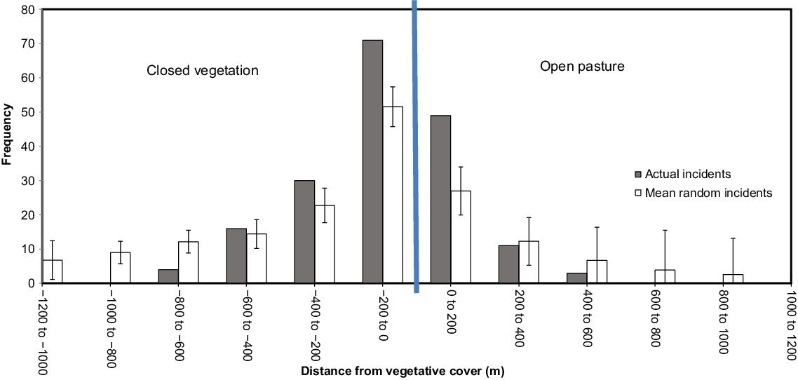
Anecdotal and observational information suggested that at the time of day the surveys were undertaken, fallow deer might congregate near the interface between vegetative cover and more open areas. This is likely to influence where in the landscape deer have the greatest impact on crops and natural values, and where control efforts may be best focused. The geographical coordinates for each individual animal in the thermal imagery allowed deer distribution in relation to vegetation structure to be formally tested at a fine scale. We calculated the shortest distance from each recorded fallow deer location to the nearest edge of the nearest GIS vector polygon of vegetative cover (hereon called ‘edges’) using Program fragstats (Lethbridge 2015). Vegetation data were sourced from the National Vegetation Information Scheme (NVIS Technical Working Group 2017). We used a histogram of deer-to-edge distances, expressed in metres, to examine the frequency at which deer were found in open versus closed vegetation (following DeBats and Lethbridge 2005). Negative values indicate deer that were found in closed vegetation, and positive values indicate open vegetation. Zero is the ‘edge’ of open and closed vegetation polygons. As the shape of this histogram may be an artefact of the landscape’s structure, the algorithm also randomly generates the same number of points as the observations (hereafter ‘N’) to simulate a mean random stochastic process. As with the observed deer, the distance from each random point was measured to the nearest edge. Multiple sets of N random points were generated in 1000 simulations to calculate the nearest distance to vegetative cover, together with a Z score and 95% Confidence Intervals (CIs). A histogram of the distances of the actual incidence of deer was then overlaid with a histogram of the mean random stochastic process for comparison.
For this analysis, the position of each animal was used directly from the thermal imagery rather than the tagged positions entered on the electronic keypads by human observers, because data entry via the electronic keypads usually incurs a minor time lag to the true position of each animal. The coordinates of each thermal detection were determined from the pixel locations of the animal in a given frame, synchronised with the flight GNSS track log. This also required the known AGL of the aircraft, as well as the camera angle and swathe width at the time the frame was captured.
Results
The point locations of the thermal detections of deer, overlaid on the observer detections of deer, are displayed in Fig. 2. Markers in Fig. 2 may represent single animals or groups of animals, and therefore indicate the observed presence or absence of deer at any given location, rather than their population density. It should be noted that the swathe of the thermal camera was 38.5 m on the ground on one side of the aircraft, whereas human observers were viewing out to a distance of 150 m on both sides of the aircraft. Greatest overlap of detections between the two methods was in the centre of the survey area, corresponding roughly with the historical range of the species. Aerial observers detected the presence of deer where thermal imagery did not at the northern, southern and western geographical extremes of the survey area (Fig. 2), presumably where deer population density was lowest.
Thermal sightings of fallow deer (red) within the aerial survey footprint, compared with aerial observer sightings (blue).
Human observer detections and Mark Recapture Distance Sampling
As a trainee was seated behind the front-left observer for ~30% of the survey, the best way to manage any biases associated with the trainee’s counts was to test ‘trainee’ as a covariate in the modelling process, in an attempt to explicitly model any biases from this person out of the results. The ‘trainee’ covariate variable has a value of ‘1’ in the models when the trainee is present in the rear-left seat and a ‘0’ when an experienced and calibrated observer was present in the rear-left seat.
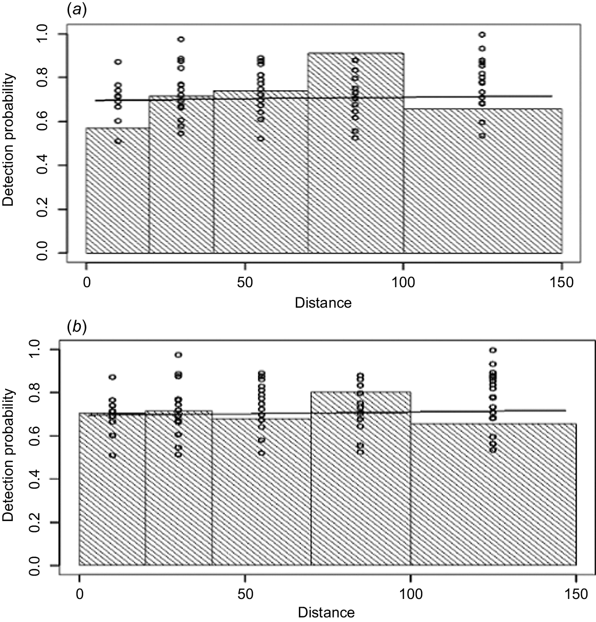
Figs 3 and 4 compare the detection probabilities and conditional probabilities that best summarise the observations of the front and rear observers. The conditional probabilities between observers (P1|2(x) and P2|1(x) in Fig. 4) are relatively flat lines and depart from the individual probability functions (P1(x) and rear P2(x) in Fig. 3). They are however, very close in magnitude at P(0). This shows some dependency between front and rear positions with distance out from the aircraft because the histograms do not follow the same shapes as in Fig. 3. This suggests using a Point Independence (PI) modelling approach, rather than a full independence modelling approach because while there appears to be independence at x = 0 (i.e. the same probabilities are apparent between Figs 3 and 4 at x = 0), the flatter lines in Fig. 5 show a positive correlation between observers, thus a full independence approach would be biased at larger distances (Borchers et al. 2006).
Comparison of the detection probabilities of the (a) front (P1(x)) and (b) rear (P2(x)) human observers with increasing distance (m).
Front detection probabilities of human observers, (a) the probability of a front seat sighting P1 given the rear P2, P1|2(x) and (b) vice versa P2|1(x) with increasing distance (m).
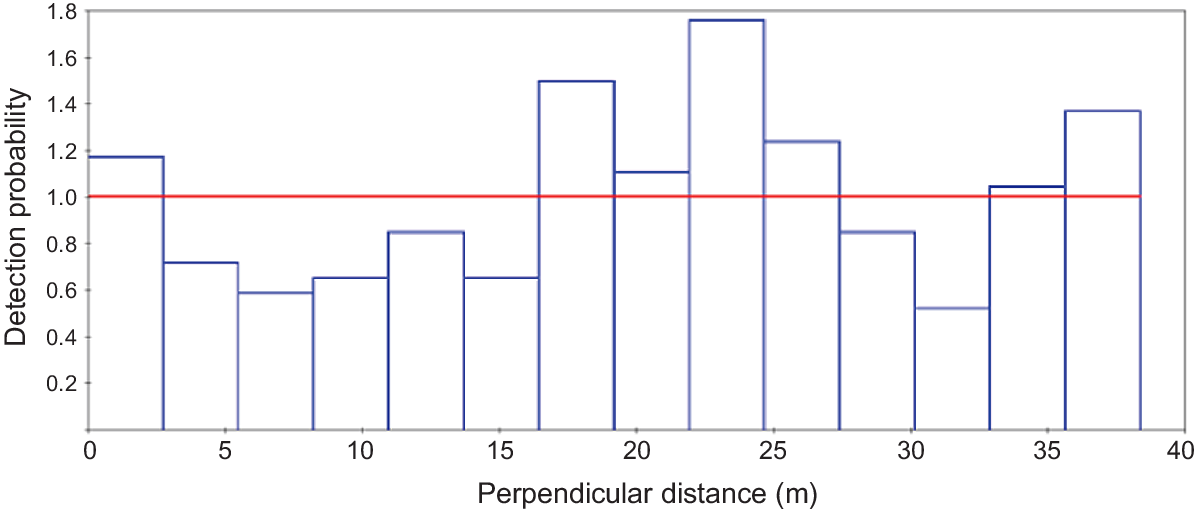
Pooled detection probabilities from human observers by distance (m), during the 2019 fallow deer survey of eastern Tasmania.
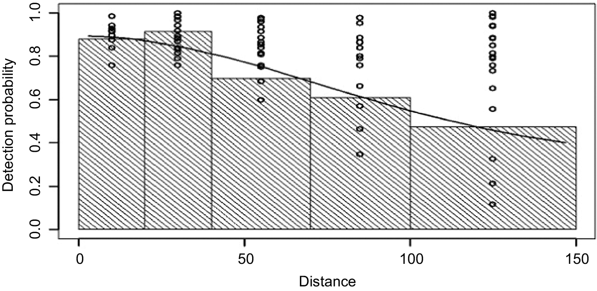
Table 1 shows the relative performance of models with each combination of covariates using the MRDS approach. We followed the approach taken by Borchers et al. (1998), whereby the DS and mark–recapture components of MRDS are both dependent. Table 1 also shows the covariates that help to explain sources of data heterogeneity. For the mark–recapture component, distance is only treated as a linear covariate of sighting probability (Becker and Christ 2015). From results in Table 1, the best scoring MRDS model with the lowest AIC score was g(x) ~ trainee + cluster size and mr() ~ trainee + cluster size + distance. The presence of a trainee was found to be important in the model, suggesting the trainee’s counts could have biased the results if not considered. Group size (cluster size) also affected sightability, with sightability increasing as herd size increased. Under the preferred model (lowest AIC), the line of best fit applied to the pooled detection probability of both left-side observers with distance suggested that the function g(x) decreased with distance out from the aircraft up to 150 m, the observation limit marked on the aircraft sighting poles (Fig. 5). Using the best-performing model in Table 1, the estimated density of fallow deer within the survey area was 2.696 deer km−2 (CV 19%; LCL 1.839; UCL 3.952). Multiplied over the entire survey area of 19,905 km−2, the human observer dataset produces an estimated population size of 53,660 deer.
Thermal detection and Multiple Covariate Distance Sampling
The preferred model for estimating deer density (Table 2) did not include covariates, suggesting that habitat (woodland versus open areas) and sun direction did not affect sightability of deer in the thermal imaging surveys. An examination of the histogram of the thermal camera sightings of fallow deer for the preferred model (model g(x) ~.) indicated that there was no decay in sightability with distance out from the aircraft (Fig. 6). The preferred model (lowest AIC) generated a density estimate of 2.821 deer per km2, with a coefficient of variation (CV) of 36%. Multiplied over the entire survey area of 19,905 km2, the thermal dataset produces an estimated population size of 56,152 deer.
| Name | AIC | ESW | D | D LCL | D UCL | D CV | |
|---|---|---|---|---|---|---|---|
| g( x) ~ . | 1570.5 | 38.4 | 2.821 | 1.400 | 5.684 | 36% | |
| g(x) ~ sun | 1570.8 | 36.0 | 3.004 | 1.509 | 5.982 | 35% | |
| g(x) ~ habitat | 1572.5 | 38.3 | 2.824 | 1.419 | 5.618 | 35% | |
| g(x) ~ habitat + sun | 1572.6 | 36.0 | 3.011 | 0.008 | NA |
Best-performing model (lowest AIC) is in bold.
AIC, Akaike’s Information Criterion; CV, coefficient of variation; D, density per km2; ESW, effective strip width; LCL, lower confidence interval; UCL, upper confidence interval.
Distribution in the landscape in relation to habitat
The histogram in Fig. 7 shows that at the time of year and times of day that the survey was conducted, fallow deer were heavily concentrated within 200 m either side of the interface between open pasture and closed vegetation. Open pasture included native or exotic pastures, and closed vegetation included native forests, woodlands and mixed shrublands. In closed vegetation, all detections of deer were within 800 m of the interface with open pasture, and most were within 600 m. In open pasture, all detections were within 600 m of the habitat interface with closed vegetation, and most were within 200 m. From 0 to 600 m inside a closed canopy, actual incidents of deer (grey bars in Fig. 7) show distribution was biased towards closed vegetation compared to the random stochastic processes (white bars in Fig. 7, along with 95% confidence intervals from Z scores), that is compared to if the deer were randomly located. In open pasture, more deer were found within 200 m of the closed canopy than would have been expected, compared to the random stochastic processes, the number within 200–400 m closely matched the random stochastic process, and fewer deer than would have been expected based on random distribution were found beyond 400 m.
Distance from geographical coordinates of deer (derived from thermal imagery) to edge of nearest vegetation cover, plotted against randomly placed points simulated 1000 times. Error bars reflect 95% Z-score. Vegetation data sourced from the National Vegetation Information Scheme (NVIS Technical Working Group 2017).
Discussion
Comparison of density estimates from human and thermal camera surveys
Both the observer and thermal survey data were collected simultaneously during the same flights to eliminate sources of variability that might arise from surveying at different times, due to animal movement and weather conditions. As the true size of the Tasmanian deer population is unknown, the two aerial survey methods must be evaluated in relative terms. We have been cautious in not conducting a statistical comparison of the two methods because they have very unequal sample sizes, due to human observers counting from both sides of the aircraft and the camera being used only on one side, and the difference is strip width between the two methods.
Nevertheless, in this survey, both methods resulted in similar population density estimates, with the human observer counts producing an estimate of 2.7 fallow deer per km2, and the thermal camera data 2.8 deer per km2. We consider that the use of thermal cameras holds potential for this type of survey in the future, but are cautious not to overstate its value based on our findings because of the much larger magnitude of uncertainty in the population density estimates from the single thermal camera (CVthermal = 36%; CVobservers = 19%). In effect, this suggests that the two density estimates may have converged by chance on this occasion given the inevitable lower sample size from a single camera with a narrow strip width, and the thermal estimate could have been much higher or much lower. The thermal estimate is not sufficiently precise to enable evidence-based management decisions for deer in Tasmania, and for now we consider human observers to be more reliable. From a cost-effectiveness perspective, the bulk of the expense of such surveys is in the cost of using a helicopter, so there would be little efficiency gain from reduced labour costs of aerial observers in favour of a camera, particularly for a lower sample size with a single camera. Future testing should incorporate two cameras, one on either side of the aircraft, to increase sample size with the aim of reducing the CV of the population density estimate.
Baseline fallow deer population density and size in Tasmania
The estimates of 2.7–2.8 deer per km2 in the present study suggest that the density of introduced fallow deer in Tasmania for 2019 was considerably lower than what has been observed for deer populations across habitats in Mediterranean (10–100 deer per km2; Ferretti et al. 2011; Ferretti and Fattorini 2021), warm temperate (50–150 deer per km2; Moody et al. 1994; Gogan et al. 2012), and temperate systems (26–50 deer per km2; Walander 2012). However, our density estimates are generalised over an area approximately 100–2,000 times larger than in other published studies (9–218 deer per km2), and encompassed areas of both high and very low deer abundance (Fig. 2).
Compared to the point estimates of density over much smaller areas in other studies (Moody et al. 1994; Gogan et al. 2012; Walander 2012), areas of very low density would have substantially reduced the overall density estimates in our study, and thereby deflated the population estimates when multiplied over the entire landscape area. This observation suggests caution is warranted when applying results from other precincts in the modelling of projected future abundance of fallow deer in Tasmania (e.g. Potts et al. 2015; Cunningham et al. 2022). Furthermore, the low average population density across the entire study area is unlikely to accurately reflect deer impacts on native ecosystems and agricultural lands where localised population densities could be much higher. Deer impact studies need to consider how evidence of a highly heterogeneous spatial distribution of deer in the landscape (Fig. 7) can be incorporated into study design.
The MRDS density estimate based on our human observer survey data produced an estimated population size of approximately 53,660 fallow deer in central and north-eastern Tasmania for 2019. Given that approximately 30,000 deer were removed prior to the survey through hunting and under crop protection permits, this suggests that the total estimated population for Tasmania for 2019 may have been in excess of 83,000 individuals. In other words, ignoring population growth rates, around one-third of the population was likely removed through hunting and control permits in 2019. These baseline figures provide a benchmark for future surveys, and for understanding what the population trajectory might otherwise have been without control measures.
Localised distribution of deer in relation to habitat
Using the precise geographical coordinates for each individual deer available from the thermal imaging data, we were able to investigate localised deer distribution in relation to habitat. Overlaying these coordinates on GIS vegetation data, we were able to quantify the preference of deer for ecotone habitats in Tasmania at the time of year the survey was conducted (Fig. 7). Deer were primarily found within a few hundred metres of the interface between closed vegetation and an open pasture, with the majority found within 200 m, and with significantly more deer concentrated near this interface when compared to the random stochastic process.
A preference for ecotone habitats has been noted for several species of deer in other locations (McLoughlin et al. 2007; Miyashita et al. 2008; Massé and Côté 2009; Ferretti et al. 2011; Wuensch et al. 2023), including fallow deer (Braza and Álvarez 1987; Borkowski and Pudełko 2007; Liu and Nieuwenhuis 2014; Davis et al. 2023). This may relate to the need for herbivores to make a trade-off between access to the more abundant resources available within open habitats (e.g. pastures, grasslands), and an increased predation risk through loss of lateral cover (Lima and Dill 1990; Tufto et al. 1996; Verdolin 2006; Owen-Smith 2014).
Confirmation that fallow deer were congregated near the interface of open and closed habitats in Tasmania at this time of year could be used to develop more efficient survey and management methods. We did not explore other aspects of habitat associated with deer presence or abundance, such as vegetation type, patch shape and size, or level of fragmentation of the closed native and plantation vegetation communities, and this could be a fruitful avenue for further investigation. Landscape metrics have been used in conservation planning to measure species responses to fragmentation (e.g. McGarigal et al. 2002; Lethbridge et al. 2010), but to date this has not been applied to overabundant or pest species. Should more expansive distribution models be developed for fallow deer in Tasmania, incorporating features such as landscape structure and fragmentation may allow more targeted control and impact monitoring. However, we stress that broadscale monitoring of deer geographical distribution will remain important for preventing their expansion into new areas, as in the long term it is most effective and cost-efficient to control new populations early in the invasion curve (Department of Primary Industries 2010).
For the purposes of planning, it should be noted that our study did not characterise deer habitat use at other times of year, and there may be relevant differences in habitat use by season and by sex. For example, use of closed habitats is known to vary at different times of year, and males only mix with female herds from early autumn to early winter during the rut (Thirgood 1995; Apollonio et al. 1998). In our spring survey, which is after the breeding season, the observed clustering of deer within 600–800 m either side of transitions from forested to open habitats is likely explained by single-sex herds using a broad swathe of the landscape during the period of the survey. The noted breadth of habitat use will have implications for population monitoring techniques that rely on observational data if surveys are conducted during seasons when the use of forested habitat may be high.
From a conservation planning and land management perspective, a large proportion of remnant forested habitat may effectively be categorised as ecotone habitat in highly fragmented landscapes (e.g. Apollonio et al. 1998; Borkowski and Pudełko 2007; Massé and Côté 2009; Liu and Nieuwenhuis 2014). The pattern of ecotone habitat use we observed suggests careful consideration is warranted when defining what is and is not deer habitat in Tasmania, and when quantifying their habitat preferences. Studies examining the effects of deer on habitat integrity and/or agricultural production should sample across the full range of natural and modified habitats at each location, to ensure they detect and quantify all impacts. Based on our empirical observations that deer clustered near habitat transitions, it would be reasonable to hypothesise that further fragmentation of native habitats would create more transitional zones that would favour deer and could lead to population expansion or concentration.
Technical improvements
In addition to our earlier observations about use of a single camera, the lack of sightability decay in the thermal imagery (Fig. 6) is a further indication that using a single thermal camera configured in this way was not ideal for estimating population density in this study. The camera viewing area was a relatively small swathe (38.6 m). Given that the Effective Strip Width (ESW) was 37.1 m and the total viewing area of the camera was only 1.5 m further out from the ESW, and had no decay in the function g(x), a more robust MCDS estimate might be better attained in future by increasing the swathe. This could be achieved through (1) increasing flying height, and/or (2) decreasing the tilt on the camera to bring its field of view further towards the horizon. This would allow g(x) to decay more gracefully, with objects further out from the frame beginning to pixelate and become undetectable.
Doing this would require a higher-resolution camera. Since this study, the primary author has tested the use of two thermal cameras on helicopter and remotely piloted (uncrewed) platforms, both having a much higher resolution (1200 × 1900 pixels). This has resulted in clearer detections, enabling the cameras to be pointed further out from the aircraft, allowing g(x) to decline with perpendicular distance and therefore providing more certainty of the ESW. These results are encouraging, and with improving technology there is likely to be higher demand for thermal camera surveys for broadscale wildlife monitoring, especially using remotely piloted platforms. However, from an operational point of view, we note that at least in Australia, the low-flying operations needed for broadscale wildlife monitoring are impractical with remote platforms in most areas due to aircraft safety considerations. Low-flying remotely piloted platforms pose serious safety risks, especially if flying beyond visual line of sight – as would be required for a survey of the scale in this study – and Australia’s Civil Aviation Safety Authority requires written landholder permission before fly-over is permitted. Helicopter platforms, which are safer and require fewer permissions, therefore continue to be a more practical option for most aerial surveys of scale.
Analytical improvements
Future modelling of deer in Tasmania may benefit from integration of distance sampling into Bayesian Markov Chain Monte Carlo (MCMC), or N-mixture models. Integrated modelling has many advantages, including accounting for unmodelled heterogeneity associated with animal behaviour, largely manifesting in the encounter rate and for observer counts, group size. This is separate from modelling observation errors, which must be tested with different covariates (Hilborn and Mangel 1997). In aerial surveys these may be, for example, sun direction, canopy cover, or cloud cover. MCMC or N-mixture models attempt to separate the influences of observational biases and animal behaviour (Royle 2004), particularly when the survey can be repeated. MCMC and allied approaches have yet to be attempted for deer in Australia, but have recently been utilised for modelling waterfowl density and abundance (Ramsey and Fanson 2021). Spatial autocorrelation will also require testing as this could introduce variance inflation, or even biases when testing for deer responses to landscape features. This has recently been found to be a major factor influencing grey kangaroo distribution in fragmented habitats, along with landscape structure (Lethbridge et al. in review).
Implications for future surveys and deer management
With increasing regard for the effects of deer on Tasmania’s environment and economy (Coleman et al. 1997; Smith et al. 2012; Bailey et al. 2014; Davis et al. 2016; Driessen et al. 2020; Invasive Species Council 2021; Cunningham et al. 2022; Heaton et al. 2022), the aim of the Tasmanian Wild Fallow Deer Management Plan 2022–2027 is to deliver positive ecological, economic and social outcomes by providing for a sustainable deer population within the species’ historic range in the Tasmanian Midlands, while seeking to reduce/eradicate deer populations outside the historic range (NRE Tasmania 2022). It is anticipated that these goals will be achieved by broadening the options available to landholders to control deer on their properties, removing the constraints of a legislated open season and bag limits in areas outside the species’ historic range, and by undertaking active deer control on conservation lands.
Future choice of survey type for Tasmania (human observer, thermal camera, or both) will depend on cost and priorities. In our study, human observer counts resulted in more reliable counts, but this performance advantage might be outweighed if a second camera was added to the aerial platform. On this occasion thermal footage produced a less reliable, albeit very similar, density estimate but also demonstrated the analytical potential of precise geospatial data for understanding deer habitat use. Increased sample size would take full advantage of this potential by allowing, for example, potential effects of spatial autocorrelation to be interrogated.
Aerial culling from helicopters is a common method of reducing populations of invasive vertebrates, with ongoing improvements being sought to the efficiency and ethicality of operations (Hampton et al. 2021), but this is subject to diminishing returns as density declines (Fattorini et al. 2020; Bengsen et al. 2023). With populations of large, introduced herbivore species requiring routine management, additional improvements should be investigated to reduce long-term costs. Further efficiencies, at least during spring, could be generated if flight plans initially focused on edge habitats in order to target deer that are preferentially utilising this habitat, before initiating random or grid-based search patterns in other areas. Other deer control mechanisms (e.g. ground shooting, Bengsen et al. 2020; poisoned bait programs, McKenzie et al. 2022) might also benefit from prioritising edge habitats in the first instance.
Data availability
The raw data for this study are held by the Department of Natural Resources and Environment Tasmania and are not publicly available. Queries about the data and analysis should be directed to the corresponding author.
Declaration of funding
Collection of the aerial survey data used in this study was funded by the Department of Natural Resources and Environment Tasmania as part of routine wildlife monitoring. The analysis for the research publication did not receive any specific funding.
References
Akaike H (1974) A new look at the statistical model identification. IEEE Transactions on Automatic Control 19, 716-723.
| Crossref | Google Scholar |
Apollonio M, Focardi S, Toso S, Nacci L (1998) Habitat selection and group formation pattern of fallow deer Dama dama in a sub mediterranean environment. Ecography 21, 225-234.
| Crossref | Google Scholar |
Bailey TG, Gauli A, Tilyard P, Davidson NJ, Potts BM (2014) Feral deer damage in Tasmanian restoration plantings. Australasian Plant Conservation: Journal of the Australian Network for Plant Conservation 23, 10-12.
| Crossref | Google Scholar |
Becker EF, Christ AM (2015) A unimodal model for double observer distance sampling surveys. PLoS ONE 10, e0136403.
| Crossref | Google Scholar | PubMed |
Bengsen AJ, Forsyth DM, Harris S, Latham ADM, McLeod SR, Pople A (2020) A systematic review of ground-based shooting to control overabundant mammal populations. Wildlife Research 47, 197-207.
| Crossref | Google Scholar |
Bengsen AJ, Forsyth DM, Pople A, Brennan M, Amos M, Leeson M, Cox TE, Gray B, Orgill O, Hampton JO, Crittle T, Haebich K (2023) Effectiveness and costs of helicopter-based shooting of deer. Wildlife Research 50, 617-631.
| Crossref | Google Scholar |
Borchers DL, Zucchini W, Fewster RM (1998) Mark–recapture models for line transect surveys. Biometrics 54, 1207-1220.
| Crossref | Google Scholar |
Borchers DL, Laake JL, Southwell C, Paxton CGM (2006) Accommodating unmodeled heterogeneity in double-observer distance sampling surveys. Biometrics 62(2), 372-378.
| Crossref | Google Scholar |
Borkowski J, Pudełko M (2007) Forest habitat use and home-range size in radio-collared fallow deer. Annales Zoologici Fennici 44, 107-114.
| Google Scholar |
Braza F, Álvarez F (1987) Habitat use by red deer and fallow deer in Doñana National Park. Miscellània Zoològica 11, 363-367.
| Google Scholar |
Buckland ST, Elston DA (1993) Empirical models for the spatial distribution of wildlife. Journal of Applied Ecology 30(3), 478-495.
| Crossref | Google Scholar |
Canaval S (2014) The story of the fallow deer: an exotic aspect of British globalisation. Environment and Nature in New Zealand 9, 37-60.
| Google Scholar |
Carpio AJ, Guerrero-Casado J, Barasona JA, Tortosa FS, Vicente J, Hillstrom L, Delibes-Mateos M (2017) Hunting as a source of alien species: a European review. Biological Invasions 19, 1197-1211.
| Crossref | Google Scholar |
Chrétien L-P, Théau J, Ménard P (2015) Wildlife multispecies remote sensing using visible and thermal infrared imagery acquired from an unmanned aerial vehicle (UAV). The International Archives of the Photogrammetry, Remote Sensing and Spatial Information Sciences XL-1-W4, 241-248.
| Crossref | Google Scholar |
Crowley SL, Hinchliffe S, McDonald RA (2017) Conflict in invasive species management. Frontiers in Ecology and the Environment 15, 133-141.
| Crossref | Google Scholar |
Cunningham CX, Perry GLW, Bowman DMJS, Forsyth DM, Driessen MM, Appleby M, Brook BW, Hocking G, Buettel JC, French BJ, Hamer R, Bryant SL, Taylor M, Gardiner R, Proft K, Scoleri VP, Chiu-Werner A, Travers T, Thompson L, Guy T, Johnson CN (2022) Dynamics and predicted distribution of an irrupting ‘sleeper’ population: fallow deer in Tasmania. Biological Invasions 24, 1131-1147.
| Crossref | Google Scholar |
Davis NE, Bennett A, Forsyth DM, Bowman DMJS, Lefroy EC, Wood SW, Woolnough AP, West P, Hampton JO, Johnson CN (2016) A systematic review of the impacts and management of introduced deer (family Cervidae) in Australia. Wildlife Research 43, 515-532.
| Crossref | Google Scholar |
Davis NE, Forsyth DM, Bengsen AJ (2023) Diet and impacts of non-native fallow deer (Dama dama) on pastoral properties during severe drought. Wildlife Research 50(9), 701-715.
| Crossref | Google Scholar |
DeBats DA, Lethbridge M (2005) GIS and the city: nineteenth-century residential patterns. Historical Geography 33, 78-98.
| Google Scholar |
Delisle ZJ, McGovern PG, Dillman BG, Swihart RK, Sankey T, Laurin GV (2023) Imperfect detection and wildlife density estimation using aerial surveys with infrared and visible sensors. Remote Sensing in Ecology and Conservation 9(2), 222-234.
| Crossref | Google Scholar |
Department of Primary Industries (2010) Invasive plants and animals policy framework. Government of Victoria, Melbourne. Available at https://agriculture.vic.gov.au/__data/assets/pdf_file/0009/582255/Invasive-Plants-and-Animals-Framework-Sep-22.pdf
Edwards GP, Saalfeld K, Clifford B (2004) Population trend of feral camels in the Northern Territory, Australia. Wildlife Research 31, 509-517.
| Crossref | Google Scholar |
Fattorini N, Lovari S, Watson P, Putman R (2020) The scale-dependent effectiveness of wildlife management: a case study on British deer. Journal of Environmental Management 276, 111303.
| Crossref | Google Scholar | PubMed |
Ferretti F, Fattorini N (2021) Competitor densities, habitat, and weather: effects on interspecific interactions between wild deer species. Integrative Zoology 16, 670-684.
| Crossref | Google Scholar | PubMed |
Ferretti F, Bertoldi G, Sforzi A, Fattorini L (2011) Roe and fallow deer: are they compatible neighbours? European Journal of Wildlife Research 57, 775-783.
| Crossref | Google Scholar |
Focardi S, De Marinis AM, Rizzotto M, Pucci A (2001) Comparative evaluation of thermal infrared imaging and spotlighting to survey wildlife. Wildlife Society Bulletin 29, 133-139.
| Google Scholar |
Forsyth DM, Comte S, Davis NE, Bengsen AJ, Côté SD, Hewitt DG, Morellet N, Mysterud A (2022) Methodology matters when estimating deer abundance: a global systematic review and recommendations for improvements. Journal of Wildlife Management 86, e22207.
| Google Scholar |
Gogan PJ, Gates NB, Lubow BC, Pettit S (2012) Aerial survey estimates of fallow deer abundance. California Fish and Game 98, 135-147.
| Google Scholar |
Gonzalez L, Montes G, Puig E, Johnson S, Mengersen K, Gaston K (2016) Unmanned Aerial Vehicles (UAVs) and artificial intelligence revolutionizing wildlife monitoring and conservation. Sensors 16, 97.
| Crossref | Google Scholar | PubMed |
Graves HB, Bellis ED, Knuth WM (1972) Censusing white-tailed deer by airborne thermal infrared imagery. The Journal of Wildlife Management 36, 875-884.
| Crossref | Google Scholar |
Hampton JO, Bengsen AJ, Pople A, Brennan M, Leeson M, Forsyth DM (2021) Animal welfare outcomes of helicopter-based shooting of deer in Australia. Wildlife Research 49, 264-273.
| Crossref | Google Scholar |
Heaton DJ, McHenry MT, Kirkpatrick JB (2022) The fire and fodder reversal phenomenon: vertebrate herbivore activity in burned and unburned Tasmanian ecosystems. Fire 5, 111.
| Crossref | Google Scholar |
Huaman JL, Helbig KJ, Carvalho TG, Doyle M, Hampton J, Forsyth DM, Pople AR, Pacioni C, Nugent G (2023) A review of viral and parasitic infections in wild deer in Australia with relevance to livestock and human health. Wildlife Research 50, 593-602.
| Crossref | Google Scholar |
Kaminski DJ, Harms TM, Coffey JM (2019) Using spotlight observations to predict resource selection and abundance for white-tailed deer. Journal of Wildlife Management 83, 1565-1580.
| Google Scholar |
Laake J, Dawson MJ, Hone J (2008) Visibility bias in aerial survey: mark–recapture, line-transect or both? Wildlife Research 35, 299-309.
| Crossref | Google Scholar |
Larson DL, Phillips-Mao L, Quiram G, Sharpe L, Stark R, Sugita S, Weiler A (2011) A framework for sustainable invasive species management: environmental, social, and economic objectives. Journal of Environmental Management 92, 14-22.
| Crossref | Google Scholar | PubMed |
Lethbridge MR, Alexander PJ (2008) Comparing population growth rates using weighted bootstrapping: guiding the conservation management of Petrogale xanthopus xanthopus (yellow-footed rock-wallaby). Biological Conservation 141, 1185-1195.
| Crossref | Google Scholar |
Lethbridge MR, Westphal MI, Possingham HP, Harper ML, Souter NJ, Anderson N (2010) Optimal restoration of altered habitats. Environmental Modelling & Software 25(6), 737-746.
| Crossref | Google Scholar |
Lethbridge M, Stead M, Wells C (2019) Estimating kangaroo density by aerial survey: a comparison of thermal cameras with human observers. Wildlife Research 46, 639-648.
| Crossref | Google Scholar |
Lima SL, Dill LM (1990) Behavioral decisions made under the risk of predation: a review and prospectus. Canadian Journal of Zoology 68, 619-640.
| Crossref | Google Scholar |
Liu Y, Nieuwenhuis M (2014) An analysis of habitat-use patterns of fallow and sika deer based on culling data from two estates in Co. Wicklow. Irish Forestry 71, 27-49.
| Google Scholar |
Marsh H, Sinclair DF (1989) Correcting for visibility bias in strip transect aerial surveys of aquatic fauna. The Journal of Wildlife Management 53(4), 1017-1024.
| Crossref | Google Scholar |
Massé A, Côté SD (2009) Habitat selection of a large herbivore at high density and without predation: trade-off between forage and cover? Journal of Mammalogy 90, 961-970.
| Crossref | Google Scholar |
McGarigal K, Cushman SA, Neel MC, Ene E (2002) FRAGSTATS: spatial pattern analysis program for categorical maps. Available at http://www.umass.edu/landeco/research/fragstats/fragstats.html [accessed 16 January 2023]
McKenzie J, Korcz M, Page B, Wiebkin A, Marcus J (2022) Feral deer aggregator: final report for project P01-T-001. (Centre for Invasive Species Solutions) Available at https://pestsmart.org.au/wp-content/uploads/sites/3/2023/10/T001-Final-release.pdf [accessed December 2023]
McLoughlin PD, Gaillard J-M, Boyce MS, Bonenfant C, Messier F, Duncan P, Delorme D, Moorter BV, Said S, Klein F (2007) Lifetime reproductive success and composition of the home range in a large herbivore. Ecology 88, 3192-3201.
| Crossref | Google Scholar | PubMed |
Miyashita T, Suzuki M, Ando D, Fujita G, Ochiai K, Asada M (2008) Forest edge creates small-scale variation in reproductive rate of sika deer. Population Ecology 50, 111-120.
| Crossref | Google Scholar |
Moriarty A (2004) The liberation, distribution, abundance and management of wild deer in Australia. Wildlife Research 31, 291-299.
| Crossref | Google Scholar |
Owen-Smith N (2014) Spatial ecology of large herbivore populations. Ecography 37, 416-430.
| Crossref | Google Scholar |
Pollock KH, Kendall WL (1987) Visibility bias in aerial surveys: a review of estimation procedures. The Journal of Wildlife Management 51, 502-509.
| Crossref | Google Scholar |
Pople AR, Phinn SR, Menke N, Grigg GC, Possingham HP, McAlpine C (2007) Spatial patterns of kangaroo density across the South Australian pastoral zone over 26 years: aggregation during drought and suggestions of long distance movement. Journal of Applied Ecology 44, 1068-1079.
| Crossref | Google Scholar |
Potts JM, Beeton NJ, Bowman DMJS, Williamson GJ, Lefroy EC, Johnson CN (2015) Predicting the future range and abundance of fallow deer in Tasmania, Australia. Wildlife Research 41, 633-640.
| Crossref | Google Scholar |
Reddiex B, Forsyth DM, McDonald-Madden E, Einoder LD, Griffioen PA, Chick RR, Robley AJ (2006) Control of pest mammals for biodiversity protection in Australia. I. Patterns of control and monitoring. Wildlife Research 33, 691-709.
| Crossref | Google Scholar |
Redpath SM, Young J, Evely A, Adams WM, Sutherland WJ, Whitehouse A, Amar A, Lambert RA, Linnell JDC, Watt A, Gutiérrez RJ (2013) Understanding and managing conservation conflicts. Trends in Ecology & Evolution 28, 100-109.
| Crossref | Google Scholar | PubMed |
Royle JA (2004) N-Mixture models for estimating population size from spatially replicated counts. Biometrics 60, 108-115.
| Crossref | Google Scholar | PubMed |
Samuel MD, Garton EO, Schlegel MW, Carson RG (1987) Visibility bias during aerial surveys of elk in northcentral Idaho. The Journal of Wildlife Management 51(3), 622-630.
| Crossref | Google Scholar |
Seymour AC, Dale J, Hammill M, Halpin PN, Johnston DW (2017) Automated detection and enumeration of marine wildlife using unmanned aircraft systems (UAS) and thermal imagery. Scientific Reports 7, 45127.
| Crossref | Google Scholar | PubMed |
Smith RW, Statham M, Norton TW, Rawnsley RP, Statham HL, Gracie AJ, Donaghy DJ (2012) Effects of wildlife grazing on the production, ground cover and plant species composition of an established perennial pasture in the Midlands region, Tasmania. Wildlife Research 39, 123-136.
| Crossref | Google Scholar |
Sudholz A, Denman S, Pople A, Brennan M, Amos M, Hamilton G (2021) A comparison of manual and automated detection of rusa deer (Rusa timorensis) from RPAS-derived thermal imagery. Wildlife Research 49, 46-53.
| Crossref | Google Scholar |
Thirgood SJ (1995) The effects of sex, season and habitat availability on patterns of habitat use by fallow deer (Dama dama). Journal of Zoology 235, 645-659.
| Crossref | Google Scholar |
Thomas L, Buckland ST, Rexstad EA, Laake JL, Strindberg S, Hedley SL, Bishop JRB, Marques TA, Burnham KP (2010) Distance software: design and analysis of distance sampling surveys for estimating population size. Journal of Applied Ecology 47, 5-14.
| Crossref | Google Scholar | PubMed |
Tufto J, Andersen R, Linnell J (1996) Habitat use and ecological correlates of home range size in a small cervid: the roe deer. The Journal of Animal Ecology 65, 715-724.
| Crossref | Google Scholar |
Verdolin JL (2006) Meta-analysis of foraging and predation risk trade-offs in terrestrial systems. Behavioral Ecology and Sociobiology 60, 457-464.
| Crossref | Google Scholar |
Walter MJ, Hone J (2003) A comparison of 3 aerial survey techniques to estimate wild horse abundance in the Australian Alps. Wildlife Society Bulletin 2003, 1138-1149.
| Google Scholar |
Wuensch MA, Pratt AM, Ward D (2023) Using activity densities as an alternative approach to measuring ungulate giving-up densities in the presence of non-target species. Behavioral Ecology and Sociobiology 77, 9.
| Crossref | Google Scholar |