Predicting terrain-induced wind turbulence for smokejumper parachute operations
Natalie Wagenbrenner A * , Loren Atwood A , Jason Forthofer A and Isaac Grenfell AA
Abstract
Terrain-induced turbulence is dangerous for smokejumpers parachuting into complex terrain and results in numerous serious accidents annually.
We quantify wind modelling system WindNinja’s ability to reproduce terrain-induced effects on the mean wind speed and turbulence in complex terrain. We assess WindNinja’s suitability for use in identifying safe jump spots during smokejumper operations in complex terrain.
We evaluate the model’s ability to reproduce mean wind speed, mean wind direction and turbulence kinetic energy (TKE) measured by sonic anemometers and lidar scanners over a ridge–valley–ridge system collected under near-neutral atmospheric conditions during the Perdigão field campaign. We conduct a WindNinja simulation to examine the wind and turbulence conditions during the 2021 Eicks Fire smokejumper accident.
WindNinja can reproduce both mean wind speed and turbulence characteristics induced by the terrain. WindNinja revealed critical turbulence information that could have been useful to smokejumpers during the Eicks Fire jumping operation.
WindNinja’s ability to reproduce key features in the mean wind speed and turbulence fields induced by the terrain make it suitable for use as an aid in identifying safe jump spots in complex terrain.
Findings from this work will reduce parachute accidents and increase the safety of aerial firefighter operations.
Keywords: CFD, computational fluid dynamics, high-resolution wind, parachute operations, smokejumper, TKE, turbulence, turbulence kinetic energy, wind modelling, wind speed, WindNinja.
Introduction
Turbulence is ubiquitous in the atmospheric boundary layer (ABL). Turbulence is produced from mechanical forces, such as wind shear at the ground or over obstacles (e.g. vegetation, buildings or terrain features) and buoyant forces, such as solar surface heating and thermal plume injections from fires, industrial stacks, or other heat sources. We perceive the effects of turbulence when we experience ‘rough’ air jostling an aircraft, see a flag waving in the wind, or observe the rolling motions of a wildland fire plume. Often, ABL turbulence is not easily observed, however. Unlike in a river where we can see an eddy that forms behind a rock, we are not always able to see the turbulent eddies that develop in the wake of a mountain. Predictions of the production and distribution of turbulence in the ABL are important, because, in many cases, turbulence cannot be perceived directly by observers.
Estimates of near-surface ABL turbulence are important for many aspects of the wildland fire environment. Heilman (2023) reviewed the state of knowledge regarding the role of turbulence in wildland fire behaviour. The review showed that firebrand production and transport (Clark et al. 2020), fire spread (Finney et al. 2015; Simpson et al. 2016) and fire whirl development (Countryman 1971; Seto and Clements 2011) are all thought to be highly sensitive to the level of turbulence in the ABL. Turbulence also impacts aerial firefighting operations. Smokejumper operations are particularly sensitive to near-ground turbulence and are the subject of the present work.
Smokejumpers are wildland firefighters who parachute from low-flying aircraft, typically exiting the aircraft at 915 m (3000 feet) above ground level (AGL) to a designated landing zone, referred to as a ‘jump spot’ near a fire. They are often dispatched to remote fires in rugged terrain that are difficult to access by other means. Smokejumpers are employed by the United States Department of Agriculture (USDA) Forest Service and the Department of Interior (DOI) Bureau of Land Management (BLM), with bases located throughout the western US and Alaska. These smokejumpers use Ram-Air style parachutes, which require forward speed to maintain lift (USDA Forest Service 2018). Small wind fluctuations can drastically impact parachute aerodynamics (Balaji et al. 2005) and the ability of the smokejumper to fly the parachute effectively. Existing protocols to assess ABL turbulence during jump operations include the release of weighted streamers to visually assess winds and turbulence throughout the intended jump profile prior to the jump (USDA Forest Service 2018). Turbulence near the ground is of particular concern. Numerous hard landings, serious accidents and fatalities have been attributed to unexpected near-surface turbulence during training and operational jumps (Wildland Fire Lessons Learned Center - Fire Smokejumper Fatality - Organizational Report; https://lessons.fs2c.usda.gov/incident/eicks-fire-smokejumping-accidentfatality-2021). There was an average of four serious jump injuries per year, including one fatality, during 2015–2023 in which turbulence potentially played a factor according to accident reports from the Wildland Fire Lessons Learned Center (https://lessons.fs2c.usda.gov/).
Flow separation over ridges can create large wake zones with increased turbulence that extend far downwind. This phenomenon likely contributed to the hard landing that resulted in a smokejumper fatality during a jump on the Eicks Fire in New Mexico in 2021 (Wildland Fire Lessons Learned Center - Fire Smokejumper Fatality - Technical Report; https://lessons.fs2c.usda.gov/incident/eicks-fire-smokejumping-accident-fatality-2021). Our research team used a high-resolution diagnostic wind model developed for operational wildland fire applications, WindNinja (Forthofer et al. 2014a, 2014b; Wagenbrenner et al. 2019), to investigate surface winds and turbulence during the jump operation on the Eicks Fire. The findings indicate that the jump operation took place in the wake of a tall upwind ridge that created a large re-circulation zone characterised by regions of enhanced turbulence. These findings demonstrate that real-time forecasting of turbulence, used in conjunction with existing protocols, could assist in assessing suitable jump spots in complex terrain (Wildland Fire Lessons Learned Center - Fire Smokejumper Fatality - Technical Report; https://lessons.fs2c.usda.gov/incident/eicks-fire-smokejumping-accident-fatality-2021).
In this work, we investigate the capabilities of WindNinja, an existing wind modelling system used operationally on wildland fires, to provide real-time estimates of turbulence characteristics for smokejumper operations in complex terrain. WindNinja is widely used by fire managers in the US and around the world. It is routinely used to drive operational fire spread models such as FlamMap (Finney 2006) and Prometheus (Tymstra et al. 2010), create high-resolution hindcasts for accident investigations and plan fuel treatments and burnout operations (Drury et al. 2016), and for situational awareness. These examples utilise mean wind speed and direction predictions from WindNinja; however, WindNinja can also generate additional information about the near-surface atmosphere, such as turbulence and shear. To-date, these capabilities have not been made accessible to end users or formally assessed for accuracy by the development team.
WindNinja has previously been evaluated with field data collected over isolated hills and mountains of varying terrain complexity (Forthofer et al. 2014a, 2014b; Wagenbrenner et al. 2016, 2019); however, smokejumper operations often occur in areas with more rugged terrain. Butler et al. (2015) described wind observations taken in the Salmon River canyon of Idaho as a follow-up study to our isolated hill work with higher terrain complexity for continued model evaluation; however, this site offers the opposite extreme, with a landscape characterised by severely dissected, rugged terrain with tall, steep ridges and local-scale flows that are typically decoupled from the large-scale flow aloft. Wind modelling in the Salmon River canyon is challenging and often requires sophisticated treatment of both dynamically driven and thermally driven winds at multiple scales (Butler et al. 2015; Wagenbrenner et al. 2018). In the present study, we choose a dataset collected from a site that offers terrain complexity between that of the isolated mountains used in our previous model evaluation work and the rugged terrain of the Idaho Salmon River Canyon.
Here, we use mean wind speeed and turbulence data collected during the well-known Perdigão experiment (Mann et al. 2017; Fernando et al. 2019) to evaluate WindNinja near-surface mean wind and turbulence predictions. The Perdigão field site provides an observational wind dataset over two parallel ridges in which turbulence is characterised by a dense network of sonic anemometers and scanning lidar systems. The ridges are steep enough to cause flow separation, and signatures of the associated flow recirculation and enhanced turbulence are contained in the observational data. Additionally, the approach flow conditions are well-defined, which facilitates setting appropriate model boundary conditions and better assessment of model performance by minimising the conflation of boundary condition errors with model errors. This constitutes the first evaluation of turbulence predictions from WindNinja and extends model validation from the previous work over simpler isolated terrain features, to a slightly more complex ridge–valley–ridge system.
The objectives of this work are to (1) quantify the accuracy of mean wind speed and turbulence kinetic energy (TKE) predictions from WindNinja over a ridge-valley-ridge system under near neutral atmospheric stability; (2) assess the turbulence energy spectra over the ridge–valley–ridge system; (3) investigate the mean velocity fluctuation as a turbulence metric; and (4) present the Eicks Fire wind simulations as a real-world use case to demonstrate the potential utility of such a tool for smokejumper operations. We describe how the findings could be incorporated into a new WindNinja user interface with output products specifically targeted to support smokejumping operations.
Methods
In this work, we focus on near-ground, mechanically induced ABL turbulence, specifically, turbulence occurring in the lee of terrain features in wake zones because these areas have been observed by smokejumpers to be hazardous. Although buoyancy-driven sources are frequently present to some degree during smokejumper operations, they can often be considered negligible compared with the mechanical production of turbulence induced by the terrain. Two sources of buoyancy-induced turbulence are heat release from the fire itself and solar surface heating. However, smokejumpers typically jump far enough away from the fire that fire-generated turbulence is insignificant. Additionally, jumping operations are frequently conducted under surface winds of 3–6 m s–1, which is sufficient to disrupt convective boundary layer growth in complex terrain (Whiteman 2000). For these reasons, we do not consider buoyancy-produced turbulence here and limit this investigation to near-neutral atmospheric stability conditions. Additionally, WindNinja is formulated to perform best in neutral-stability atmospheres and so offers the most potential benefit to jumpers under these conditions.
Perdigão field observations
We evaluate modelled mean winds and TKE against data collected from the Perdigão field campaign, which took place in Portugal during 2017 (Mann et al. 2017; Fernando et al. 2019; WindsP Web Application 2020). The field site is characterised by two parallel ridges oriented northwest to southeast, forming a ridge–valley–ridge system (Fig. 1). The ridges are approximately 4 km long with slopes of ~35%. The ridgetops rise 200–250 m above the valley floor, with a ridge-to-ridge distance of 1.4 km. The surrounding terrain to the southwest and northeast is relatively flat compared with the ridge–valley–ridge system. The site is covered by patches of pine and eucalyptus trees with grass and shrub vegetation in between. Vasiljević et al. (2017) provide an in-depth description of the terrain and vegetation including photos of the site. There is a 2 MW wind turbine with a hub height of 78 m and rotor diameter of 82 m located on the southwest ridge near tower tse04 (Fig. 1). We describe possible effects of the turbine on the observation network and implications for interpretation of results in the Results and Discussion sections. Interestingly, Tomaszewski et al. (2018) investigated how turbulence induced by a wind turbine could pose a hazard to small aircraft. Although not the focus of this study, it is worth noting that wind turbines and other large bluff bodies also have the potential to produce turbulence hazards to aviation resources.
Perdigão field site and tower locations used in this study. Tower rsw06 is the calibration tower. Solid black lines indicate Transect A and Transect B, which approximately intersect the towers. The mean wind direction is from the southwest and aligned with the transects. The inset depicts the broader area; the field site is indicated with a red star.
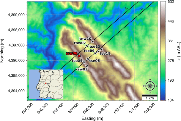
We focus on a meteorological period with steady southwest winds approximately perpendicular to the ridges. Wind speed, wind direction and TKE were measured along two transects in the streamwise direction spanning the ridge–valley–ridge system (Fig. 1). We use sonic anemometer data from three 100-m towers (tse04, tse09 and tse13) with measurements 10, 20, 30, 40, 60, 80 and 100 m above the ground and six 60-m towers (rsw06, tnw07, tnw10, rsw03, tse06 and tse11) with measurements at 10, 20, 30, 40 and 60 m. Tower tnw07 had additional measurements at 4, 6, 8 and 12 m. The quality-controlled, tilt-corrected 5-min and high-rate observed data were obtained from the NCAR Earth Observing Laboratory (Oncley 2021). The raw data were sampled at 20 Hz (Oncley 2019). We investigate the time period 22:00 to 22:30 UTC on 4 May 2017 as the evaluation case. Palma et al. (2020) calculated a bulk Richardson number of −0.03 for this time period, which indicates near-neutral atmospheric conditions. These conditions were prone to flow separation over the southwest ridge and formation of a recirculation zone between the two ridges (Menke et al. 2019). We choose this case to evaluate model performance under a double-ridge system exposed to a cross-flow under neutral atmospheric stability conditions and expect that findings will extend to other similar cases.
Model description and configuration
We use the WindNinja conservation of mass and momentum model described in Wagenbrenner et al. (2019) for this work. This model estimates a solution to the steady-state, incompressible Reynolds-averaged Navier-Stokes (RANS) equations.
NASA Shuttle Radar Tomography Mission (SRTM) (Earth Resources Observation and Science Center (EROS) 2017) data at 30-m resolution are used for the digital elevation model (DEM). The computational domain extends ~3 km beyond the study area in all directions and is constructed using the ‘fine’ mesh choice in WindNinja. This choice allocates 100,000 cells for the mesh using the meshing approach described in Wagenbrenner et al. (2019), which affords higher mesh resolution in the layers near the surface and coarser mesh resolution higher in the domain (Fig. 2). The near-ground horizontal and vertical cell resolution is 24 m. The domain height is 1597 m above ground level (AGL). The ‘brush’ option is used to set uniform vegetation throughout the domain corresponding to a roughness length of 0.43 m, zero-plane displacement height of 1.8 m and vegetation height of 2.3 m.
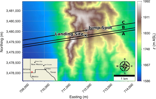
Eicks Fire terrain and jump operation points of reference. Jump Spot indicates the intended landing site. Landing Site indicates the actual landing site where the accident occurred. Transects A, B and C indicate transects sampled for wind and turbulence analysis from simulations. The mean wind direction is from the southwest, aligned with the transects. The inset depicts the broader area; the site of the jump operation is indicated with a red star.
The domain-average initialisation method in WindNinja is used. This sets the initial flow field and the boundary conditions (Wagenbrenner et al. 2019) using a logarithmic wind profile. This profile is defined by an input 10-m wind speed, wind direction and roughness parameters. The 10-m wind speed and direction are set to 2.9 m s−1 and 229° to match the calibration tower rsw06 (Fig. 1).
A sensitivity analysis was performed to investigate model sensitivity to the chosen ground roughness, mesh resolution, turbulence model and numerical discretisation schemes by independently varying each of these parameters. Results of the sensitivity analysis are presented in Appendix 1.
Model evaluation methods
We compare modelled vs observed wind speed, wind direction and TKE at the sensor locations shown in Fig. 1. Model results are discussed qualitatively, including a description of the presence and structure of key flow features throughout the domain. Model performance is also quantified in terms of the root mean square error (RMSE), mean bias error (MBE) and mean absolute percentage error (MAPE):
where φ is the observed value, φ′ is the difference between the predicted and observed and N is the number of observations. A circular mean is used for wind direction calculations.
The RANS simulation includes a transport equation for TKE and outputs TKE directly as detailed in Wagenbrenner et al. (2019). TKE is the mean kinetic energy per unit mass contained in the eddies of a turbulent flow. The measured TKE, k, is calculated from the observed 20 Hz sonic anemometer data as one half of the sum of the variances, σ2, of the velocity fluctuations:
where u′, v′, w′ are the instantaneous fluctuations about the mean and the overbar indicates the mean (e.g. u′ = u − u̅). The modelled and observed turbulence is also investigated in terms of the root-mean-square velocity fluctuations and the turbulence energy spectral density. The root-mean-square velocity fluctuations, Urms are calculated as:
We anticipate that eddies of different sizes, time scales and strengths will impact parachute flight control differently. As a first investigation into this, we examine the turbulence energy spectral density of the sonic anemometer data computed using a Fast Fourier Transform. These transformed data are plotted as the spectral density vs the associated time scale on a log-log plot to depict the energy spectrum and highlight key features of the turbulent flow. For example, the peak is associated with production of turbulence and the largest eddy sizes in the flow. We compare the energy spectral density signatures at different locations in the terrain.
Eicks fire case study
We present modelled winds and turbulence for an operational jump conducted by smokejumpers in southwest New Mexico on the afternoon of 24 May 2021 as a case study to demonstrate the potential utility of high-resolution turbulence predictions for smokejumping operations. The jump operation took place in the lee of a tall ridge exposed to a strong southwesterly wind, approximating near-neutral atmospheric conditions. The jump ended with a hard landing that resulted in a smokejumper fatality. The details of the case are published in the Eicks Fire Smokejumper Fatality Learning Review Technical Report (Wildland Fire Lessons Learned Center - Fire Smokejumper Fatality: Learning Review – Technical Report; https://lessons.fs2c.usda.gov/incident/eicks-fire-smokejumping-accident-fatality-2021) and indicate that turbulence generated from upwind terrain features likely played a role in the hard landing.
The Eicks Fire was located in the Animas Mountains of southwest New Mexico (Fig. 2). This is a high-elevation desert with rugged terrain and peaks rising over 1000 m above the valley floor. The Eicks Fire was ~20 ha in size at the time of the jump. The designated jump spot was south of the fire on a grassy slope with a west aspect (Fig. 2). Streamers released by the smokejumpers indicated west winds of ~6 m s−1 in the jump spot and the High-Resolution Rapid Refresh (HRRR) forecast modelled westerly 10-m winds of 6.2 m s−1 from 261° at the time of the jump.
A WindNinja simulation was initialised with a domain-average wind of 6.2 m s−1 from 261° at 10 m AGL to assess local winds and turbulence during jump operations.
Results and discussion
Perdigão mean wind and TKE
The modelled time-averaged wind field contains several notable flow features, including speed-up over the first ridge and flow separation over portions of both ridges with recirculation zones downwind (Figs 3 and 4). Flow speed-up occurs over sections of the second ridge that are not impacted by flow separation from the first ridge. For example, speed-up is visible over the south end of the second ridge (Fig. 3). This is likely due to the broken terrain that comprises the southern end of the first ridge, which allows flow to channel through small gaps in the terrain rather than being forced up and over the ridge. Instead of separating over the first ridge, the flow maintains its momentum as it is funnelled through the gaps in its approach to the second ridge. There is also flow channelling around the northern end of the ridges and through terrain gaps in the southern end of the ridges, visible particularly in the lower 40 m AGL plot (Fig. 3a). Flow blocking upwind of the first ridge is visible in both the 40 m and the 100 m AGL slices (Fig. 3).
Top view of the modelled flow field along terrain-following slices at (a) 40 m AGL, and (b) 100 m AGL.

Side view of the modelled flow field through (a) Transect A, and (b) Transect B. Tower labels indicate maximum sensor height for that tower.

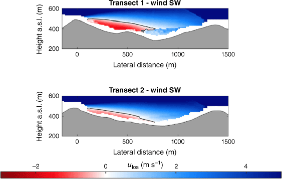
Transects A and B pass through the central portion of the ridge–valley-ridge system characterised by nearly parallel ridges of similar height without gaps in the terrain (Fig. 1). The transects pass through an area of flow separation induced by the first ridge (Figs 3 and 4). The horizontal extent of the wake region that forms behind the first ridge is approximately two times the height of the ridge and extends above and downwind of the second ridge (Fig. 4). These modelled flow separation characteristics qualitatively match the lidar observations reported in Menke et al. (2019). There is flow recirculation between the ridges along both transects (Fig. 4). Two recirculation regions can be seen along both transects, one centred immediately downwind of the upwind ridge and the other centred closer to the second ridge and slightly lower in elevation (Fig. 4). The height of the modelled recirculation region is approximately equal to the height of the first ridge and the maximum strength of the modelled reverse flow is approximately 1 m s−1 (Fig. 5). This closely matches the observed recirculation patterns reported in Menke et al. (2019) from scanning lidars during near-neutral stability southwesterly flow conditions (Fig. 6).
Modelled flow aligned with the input wind direction (229°) along (a) Transect A, and (b) Transect B. Negative values indicate reversed flow (u, wind speed).

Average line of sight (LOS) velocities observed by WindScanner lidars during southwesterly flow conditions in the Perdigão field experiment. Positive LOS velocities indicate southwesterly flow. Transect 1 and 2 correspond to Transect A and B, respectively, in this paper. Reproduced from Menke et al. (2019).
The modelled TKE field at 40 m and 100 m AGL is shown in Fig. 7. There is higher TKE at 100 m AGL compared with 40 m AGL (Fig. 7). The sensors exposed to the highest TKE in these 40 m and 100 m AGL slices are located on the second ridgetop (tnw10, tse13 and tse11; Fig. 7). This is a region of strong horizontal and vertical shear (Figs 3 and 4). The wake region from the first ridge tapers down over the second ridge and the areas with strongest TKE are located near the edges of the wake over the second ridge where horizontal shear is high (Fig. 3). There is strong vertical shear because the flow is passing over the second ridge (Fig. 4). Enhanced TKE can also be seen between the two ridges along the streamlines immediately east of tse06 (Fig. 7), which is near the edge of the wake region generated by the first ridge and a region of strong horizontal shear (Fig. 3b).
Top view of the modelled TKE field along terrain-following slices at (a) 40 m AGL, and (b) 100 m AGL.

The vertical slices (Fig. 8) show a region of enhanced TKE between the two ridges just above the recirculation zone that extends vertically and downwind just over the second ridge, following the mean flow. A similar pattern in TKE is shown in both transects, although Transect A has slightly higher TKE values.
Side view of the modelled TKE field through (a) Transect A, and (b) Transect B. Tower labels indicate maximum sensor height for that tower.

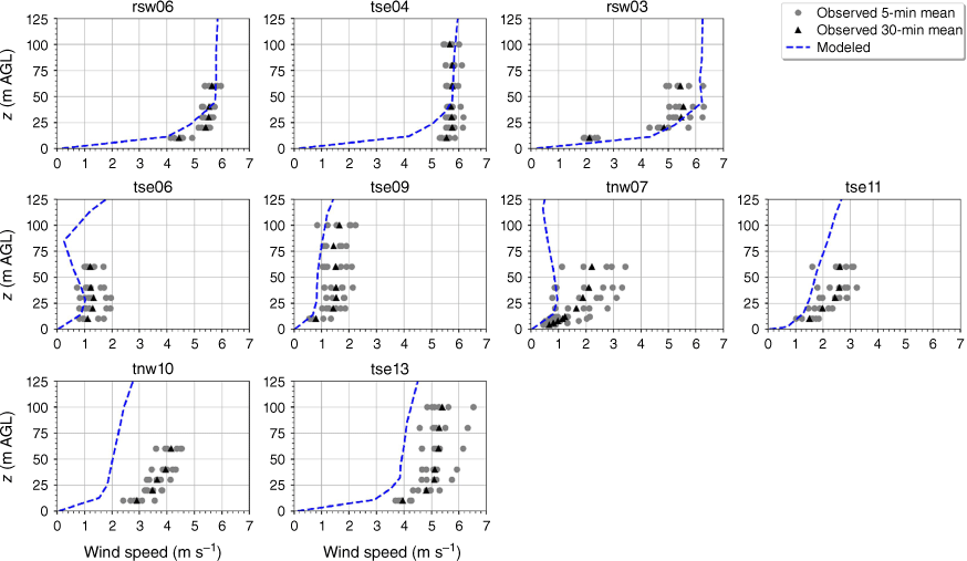
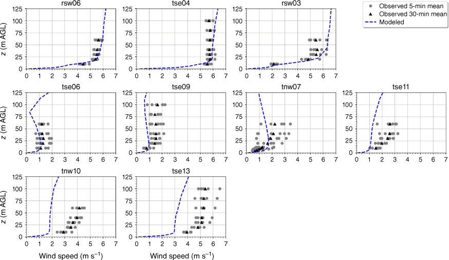
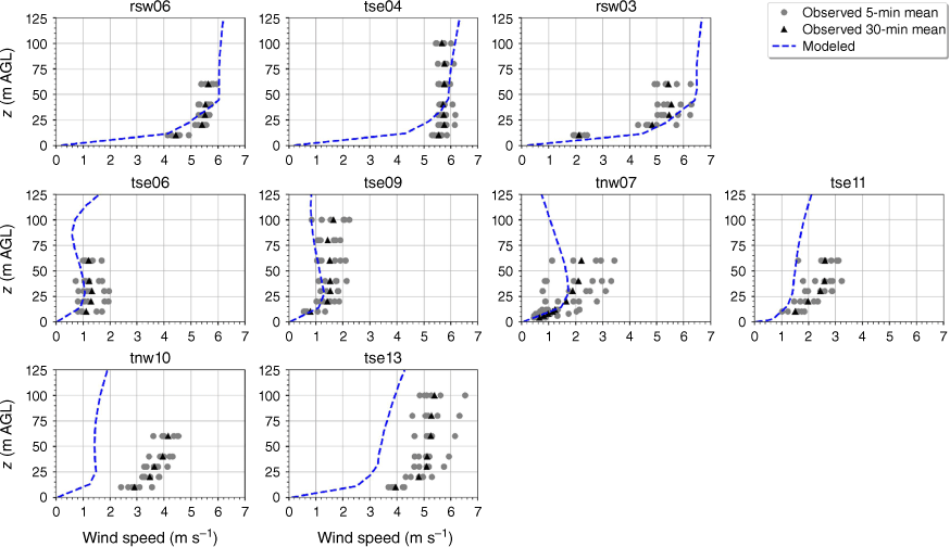
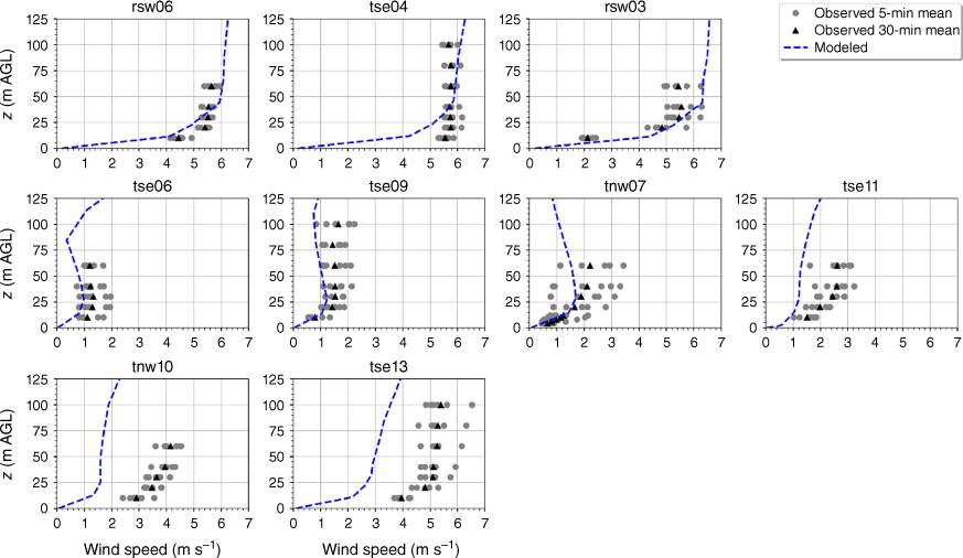
The modelled mean wind speed profile approximates the observed profile at the calibration tower, rsw06, with the modelled mean speed falling within the range of the reported 5-min mean speeds for four out of the five sensor heights (Fig. 9). The modelled speeds fall within the range of the 5-min observations for the other tower locations on the first ridge except for the lowest three heights on tower tse04 and the lowest height on tower rsw03 (Fig. 9). The model slightly underpredicts at the lowest three heights at tse04 and slightly overpredicts at the lowest height at rsw03 (Fig. 9). The modelled speed profiles slightly underpredict in the valley, but still fall within the range of the 5-min averages observed at most sensors on the valley towers (Fig. 9; tse09, tse06, tse11, tnw07). The modelled speed profile is underpredicted at the second ridge towers (Fig. 9). This could indicate that the modelled wake region from the first ridge is propagating too far downwind or perhaps is too wide as it passes over the second ridge. The wake region narrows as it approaches the second ridge, with towers tnw10 and tse13 just inside the wake region (Fig. 3). If the modelled wake region were slightly narrower over the second ridge, the wind speeds would match the observed profiles more closely.
Modelled vs observed mean wind speed at each tower. Grey circles indicate 5-min mean observations. Black triangles indicate 30-min mean observations. The top row of panels are the southwest ridge towers; the middle row of panels are the valley towers; the bottom row of panels are the northeast ridge towers.
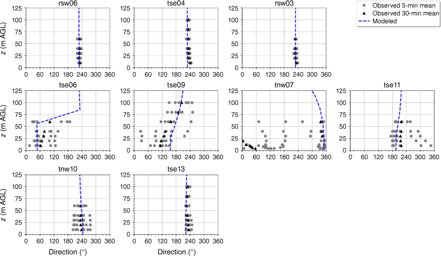
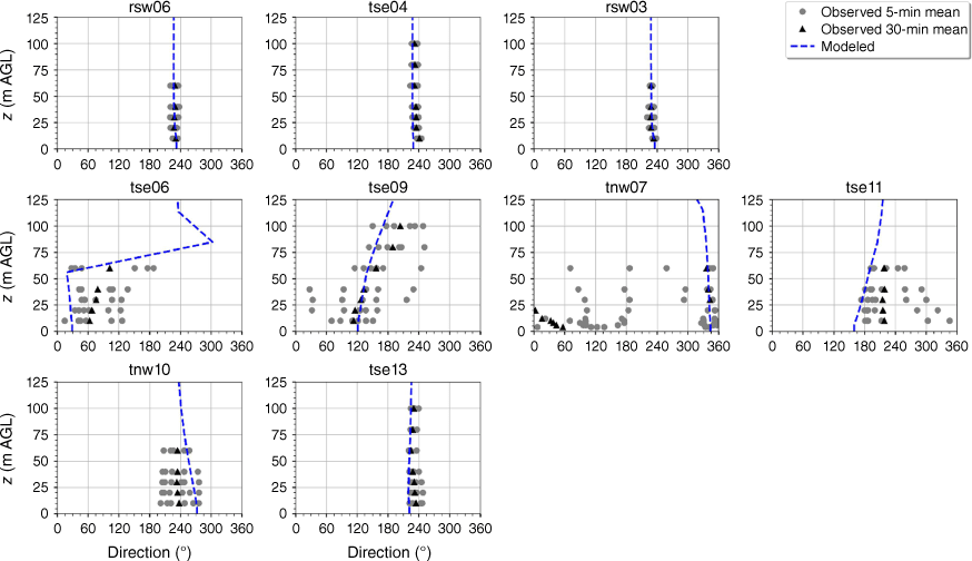
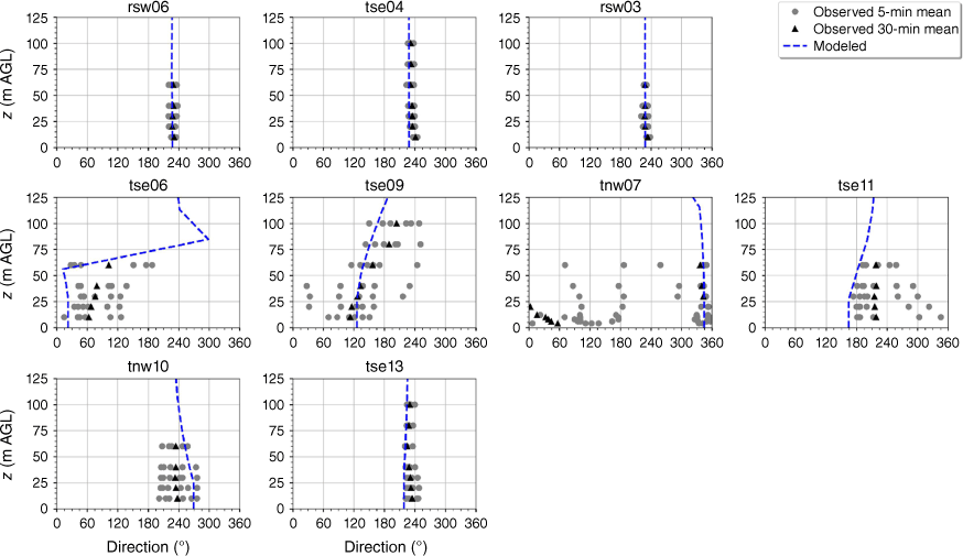
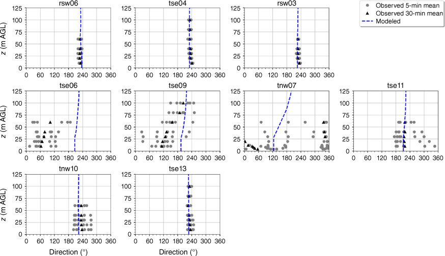
The modelled wind direction profile matches the observed wind direction profile at the calibration tower, rsw06 (Fig. 10). The modelled direction profiles closely match the observed profiles at the other two tower locations on the first ridge (Fig. 10). The wind direction observed at the first ridge is ~230°, with little vertical directional shear (Fig. 10). The observed 5-min wind directions in the valley exhibit substantial variability and the 30-min averages indicate vertical directional shear, consistent with the presence of a recirculation region (Fig. 10). The modelled direction profiles match the observed valley profiles well with all of the modelled profiles falling within the range of observed 5-min mean observations (Fig. 10). The observed direction profiles have much less variability and directional shear at towers tse13 and tnw10 on the second ridge, which suggests that these towers are outside of the turbulent recirculation region (Fig. 10). The modelled direction profiles match the observed profiles well, with all modelled directions falling within the range of the observed 5-min average directions (Fig. 10).
Modelled vs observed mean wind direction at each tower. Grey circles indicate 5-min mean observations. Black triangles indicate 30-min mean observations. The top row of panels are the southwest ridge towers; the middle row of panels are the valley towers; the bottom row of panels are the northeast ridge towers.
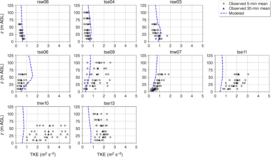
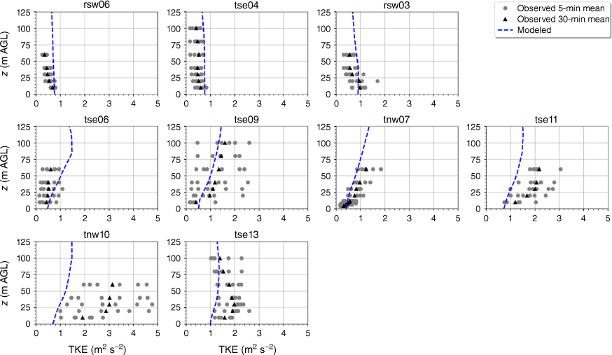
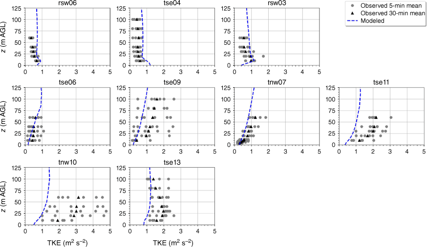
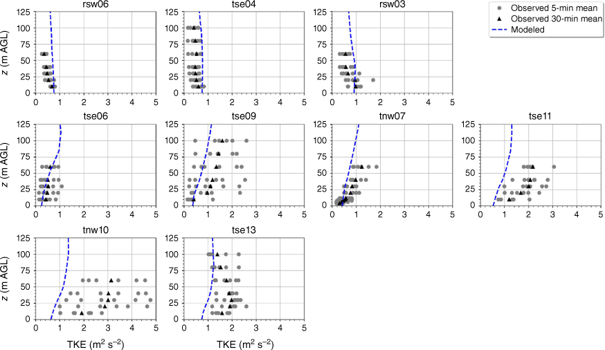
The modelled TKE is within the range of the observed 5-min mean TKE at the lower two heights of the calibration tower, rsw06 (Fig. 11). The simulation slightly overpredicts TKE at the upper three heights at rsw06 (Fig. 11). Slight overpredictions in TKE at the upper tower heights can also be seen for the towers tse04 and rsw03 on the first ridge (Fig. 11). The observed mean and variability in TKE was higher at the valley towers (Fig. 11). The modelled TKE matches the observed profiles well, with the modelled TKE falling within the range of the reported 5-min means, except for at tower tse11, where TKE is slightly underpredicted at all heights (Fig. 11). The shape of the modelled mean TKE profile closely matches the observed profiles, with TKE increasing with height (Fig. 11). The highest observed TKE values were measured at the second ridge (Fig. 11). There is also substantial variability in the observed TKE on the second ridge at tower tnw10 (Fig. 11). The simulation underpredicts TKE on the second ridge, especially at tnw10; however, the shape of the modelled TKE profiles matches the observed profiles with increasing TKE up to ~30 m and then steady or slightly decreasing TKE from 30 to 100 m (Fig. 11).
Modelled vs observed mean TKE at each tower. Grey circles indicate 5-min mean observations. Black triangles indicate 30-min mean observations. The top row of panels are the southwest ridge towers; the middle row of panels are the valley towers; the bottom row of panels are the northeast ridge towers.
As mentioned in the Methods, there was a wind turbine located on the southwest ridge near tse04. Although the turbine undoubtedly impacted near-turbine flow and turbulence downwind, we do not think it is likely that the turbine substantially affected observations at the sonic anemometers or lidar scan used in this work. We believe that the mean flow and turbulence signatures described above are induced by the terrain and only minimally impacted by the turbine. This is in line with findings reported in Wildmann et al. (2019) that showed that the turbine effect on the flow only propagates downwind ~200–400 m. Fernando et al. (2019) reported measurements with and without the turbine operating and found that the turbine only affected flow up to ~300 m downwind. Additionally, modelling by Wenz et al. (2022) found that the turbine had little effect on the flow beyond 500 m downwind or below the ridge top. They reported a well-defined wake up to 340 m downwind of the turbine that rapidly decayed beyond this distance. The turbine wake simulated by Wenz et al. (2022) under neutral atmospheric stability did not follow the terrain, but drifted upward, which compares well with the findings reported in Wildmann et al. (2019).
Characterising turbulence at Perdigão
We anticipate that different temporal and spatial scales of turbulence will impact parachute flight control differently. For example, a wind gust of very short duration, say less than 1 s, is not likely to cause loss of control as the short impulse would not change the momentum of the parachuter significantly. Similarly, a very long timescale fluctuation, say of 20-min duration, is also not likely to cause flight control difficulty as the wind changes are slow enough that the operator could adjust flight to compensate. We anticipate that turbulence of the order of seconds to minutes may be the most important timescales for parachute flight. Our analysis in previous sections focused on TKE because it is directly computed during our RANS simulation process, which uses a k-epsilon type turbulence closure, but this is a simple first-order description of turbulence. Here, we investigate more detailed turbulence characteristics and examine other potentially useful turbulence metrics for smokejumper operations.
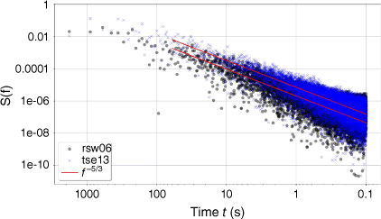
We computed the turbulence energy spectral density at two tower locations representing a location of relatively high TKE and low TKE to compare the scales of turbulence. For this purpose, 40-m data from tower rsw06 (top of the first ridge) and tower tnw10 (top of second ridge in wake from first ridge) were analysed (Fig. 12). There is a slight increase in the peak energy for tnw10 at a time scale of ~600 s compared with rsw06. The energy cascade in the inertial subrange from ~100 to 0.1 s follows the expected −5/3 power law at both locations. Eddies with time scales of ~5–10 s are anticipated to be of importance for parachute functionality, given that smokejumper flying time is ~30–60 s. As the energy spectra continuously span the temporal range relevant to smokejumpers at a known rate and scales with the peak energy, a single metric can sufficiently describe the turbulence under these atmospheric conditions.
The mean velocity fluctuation can be calculated directly from the TKE, assuming isotropic turbulence (Eqn 5). This is he mean velocity fluctuation that can be expected about the mean wind speed over time. This could be a good metric to characterise turbulence for smokejumper operations because (1) it is intuitive as it is reported in speed units and has an interpretable meaning, and (2) it indicates an absolute force affecting a parachute. Eddy dissipation rate (EDR) is a commonly used turbulence metric in the aviation industry because it is proportional to the root-mean-square vertical acceleration experienced by an aircraft (Sharman et al. 2014); however, velocity fluctuations are also frequently used to assess turbulence hazards for simple quantification and communication. Guidelines issued by the National Weather Service delineate velocity fluctuations of 1.5–5.9, 6.0–10 and 11–15 m s−1 into categories of light, moderate and severe turbulence for aircraft, respectively (National Weather Service 2024). The effect of each turbulence classification on a specific aircraft will depend on the size of the aircraft, with small aircraft being more susceptible to smaller velocity fluctuations than larger aircraft. One question is what magnitude of velocity fluctuation is sufficient to impact parachute functionality. There is not much guiding information in the literature on this topic. As the size and weight of a parachuter is much smaller than that of even a small aircraft, it is suspected that light turbulence would have a substantially larger impact on parachutes than on small aircraft. Thus, even velocity fluctuations of 1.5 m s−1 could be potentially hazardous to smokejumpers, particularly if encountered near the ground. This will likely need to be assessed, along with other turbulence metrics, including EDR, via communication with smokejumpers regarding their in-flight experiences coupled with quantification of these turbulence metrics in the jump areas.
As turbulence levels can vary drastically with elevation, one efficient way to characterise turbulence for smokejumper operations may be to quantify the maximum value of a given turbulence metric within each column of air above the terrain spanning the jump profile. This will give smokejumpers a quick estimate of the spatial distribution of the most turbulent air in their operational area. The jumpers exit the aircraft at ~915 m (3000 feet) AGL and their parachutes are deployed by 460 m (1500 feet) AGL. The region between 460 m AGL and the ground is of most importance to the smokejumpers because this is the region they are flying their parachutes in. Arguably, regions closer to the ground are more critical than regions farther away from the ground, because the closer to the ground the smokejumper is, the less room for error they have in their manoeuvres. Fig. 13 shows the maximum mean velocity fluctuation within 460 m of the ground. The largest velocity fluctuations in the study area of the Perdigão domain are found on the upwind side of the second ridge, with mean velocity fluctuations of up to 1.1 m s−1 (Fig. 13a).
Eicks fire case
A WindNinja simulation was conducted to re-create the wind and turbulence conditions during the Eicks Fire accident. Fig. 14 shows terrain-following slices of the modelled flow field at 40 m and 100 m AGL. The modelled time-averaged wind field shows flow separation over the tall ridge upwind of the landing site, indicated by the recirculation zone in the top and side views (Figs 14 and 15).
Top view of the modelled flow field along terrain-following slices at (a) 40 m AGL, and (b) 100 m AGL for the Eicks Fire domain. Jump Spot indicates the intended jump spot.

Side view of the modelled flow field through (a) Transect A, (b) Transect B, and (c) Transect C for the Eicks Fire domain. Jump Spot indicates the intended jump spot.
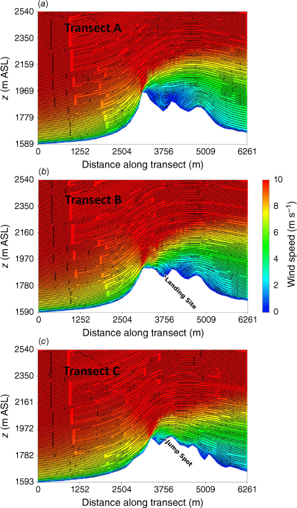
Vertical profiles of the flow were extracted along three transects aligned with the mean wind direction. Transect A runs just south of the landing site, within the northern edge of the recirculation zone (Figs 14 and 15). Transect B runs through the landing site and Transect C runs through the intended jump spot (Figs 14 and 15). Transect A runs through a tall, sharp portion of the upwind ridge and flow recirculation can be seen behind the ridge, spanning a vertical distance from the valley floor behind the ridge to the top of the ridge, ~190 m (Fig. 15a). The landing site is located behind a smoother part of the ridge with a shallower distance to the lee-side valley bottom, on the north edge of the recirculation zone. Again, the recirculation zone spans the vertical distance from the lee-side valley floor to the ridgetop, ~75 m (Fig. 15b). The intended jump spot is located further up-drainage in a shallower region of the lee-side valley and just outside of the recirculation zone (Fig. 15c).
Top and side views of the modelled TKE fields are shown in Figs 16 and 17. There is higher TKE present throughout the 100 m height surface compared with the 40 m height surface (Fig. 16). The landing site is located in an area with relatively high TKE (TKE > 3 m2 s−2 at 100 m AGL; Fig. 14b). The intended jump spot is located in an area with lower TKE than the landing site (Fig. 16). The vertical slices show a peak region in modelled TKE immediately downwind of the tall ridge, starting at approximately the height of the tall ridge and spanning a vertical distance of ~190 m above this height (Fig. 17).
Top view of the modelled TKE field along terrain-following slices at (a) 40 m AGL, and (b) 100 m AGL for the Eicks Fire domain. Jump Spot indicates the intended jump spot.

Side view of the modelled TKE field through (a) Transect A, (b) Transect B, and (c) Transect C for the Eicks Fire domain. Jump Spot indicates the intended jump spot.
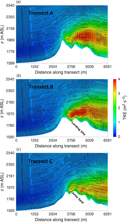
A finger of relatively high TKE can be seen in the 100 m AGL slice (Fig. 16b) extending from immediately downwind of the tall ridge, through the landing site and to the east–northeast, approximately along Transect B. This finger delineates the boundary of the recirculation zone (Fig. 16b compared with Fig. 14b). The strong gradients in the flow along this boundary are the reason for the enhanced TKE in this region and this is something smokejumpers should look out for. Enhanced turbulence can be expected along the boundaries of lee-side recirculation zones. In this case, there is a sufficiently strong gradient between the landing site and the jump spot, such that turbulence conditions are substantially different between these two locations although the distance between them is small. In the absence of turbulence forecasts, smokejumpers could watch out for strong spatial gradients in mean wind forecasts or observations, as this likely translates to increased turbulence.
Another thing to note is how far downwind the wake and enhanced TKE persist in the domain. The wake from the tall ridge and the enhanced TKE associated with this wake extend horizontally from immediately downwind of the tall ridge to beyond the eastern edge of the domain (Figs 14 and 15), 2500 m or more than six times the ridge height. Smokejumpers should be aware that terrain effects can persist far downwind, and the next ridge or two downwind of a taller exposed ridge may be in a region of very high turbulence.
The maximum velocity fluctuation was ~1.6 and 1.2 m s−1 in the column of air above the landing site and the intended jump spot, respectively (Fig. 13b). The velocity fluctuations at the landing site fall within the light turbulence rating for aircraft (National Weather Service 2024). As smokejumpers are substantially lighter than even a small aircraft, this light rating could translate to a substantial impact for their flight experience. Both TKE at 40 m and 100 m AGL and mean velocity fluctuation turbulence metrics indicate higher turbulence levesl at the landing site compared with the intended jump spot.
Implications for smokejumper jump spot assessments
WindNinja’s skill in simulating the distribution of turbulence under near-neutral atmospheric conditions at the Perdigão site suggests that it could be of use for smokejumper jump spot assessments under moderate to high wind conditions. As WindNinja is formulated for neutral atmospheric stability, model accuracy is expected to deteriorate under other stability regimes. Analyses of the energy spectral density reveal that a single metric is sufficient to characterise turbulence under these atmospheric conditions. TKE and the mean velocity fluctuation are the metrics presented in this work and are shown to correlate well with observations. It is unknown how either of these metrics correlate with parachute functionality or the ability of the smokejumper to fly. Future work is needed to assess how smokejumper in-flight experiences correlate with the various computed turbulence metrics. The EDR, which is the standard metric used in the aviation industry, should also be investigated. The turbulence metrics deemed most useful to smokejumpers could be incorporated into a turbulence forecast product customised for the smokejumper community, similar to what has been done by the National Weather Service for the aviation industry (National Weather Service Aviation Weather Center 2024). Because WindNinja is a fast-running model, with simulation times typically of the order of a few minutes, turbulence metrics could be generated in real time, for example, via a WindNinja web or mobile interface customised for the smokejumper community. Outputs such as the maximum mean velocity fluctuations or EDR in the jump column could be generated for viewing in the app. Another output that could be of use is the height AGL containing the maximum mean velocity fluctuation or EDR. Future work should evaluate relevant thresholds of EDR and mean velocity fluctuations based on smokejumper flight experiences. Specific turbulence metrics, thresholds for those metrics and display options will need to be selected based on testing and feedback from smokejumpers.
Conclusions
Mean wind and turbulence predictions from WindNinja were compared against sonic anemometer data collected during the Perdigão field campaign. Lidar data were also used for qualitative comparisons of key mean flow features. Model sensitivity to five model settings (near-ground cell size, depth of the refinement layer, roughness length, turbulence model and discretisation scheme) was investigated. Turbulence predictions were further quantified and investigated in terms of the energy spectral density and mean velocity fluctuations. A WindNinja simulation was run to re-create the wind conditions during the Eicks Fire smokejumper accident in 2021. Mean wind and turbulence predictions from this simulation were presented and discussed in the context of the smokejumper accident. The accuracy and practicality of using WindNinja to aid in identification of safe jump spots in complex terrain was discussed. Key findings from this work are:
WindNinja was able to reproduce key features in the flow field as well as spatial trends in TKE, mean wind speed and mean wind direction compared with lidar data and sonic observations under near-neutral atmospheric stability at the Perdigão field site.
WindNinja revealed enhanced turbulence at the landing site for the Eicks Fire case that likely contributed to the hard landing. There were strong gradients and wind shear along the edge of the recirculation zone, which resulted in enhanced turbulence in this region, in terms of both TKE and mean velocity fluctuations in the column up to 460 m AGL (i.e. the jump column). The velocity fluctuations modelled above the landing site fell within the light turbulence rating for aircraft (National Weather Service 2024).
Smaller ridges in the wake of tall upwind ridges can experience enhanced turbulence. Smokejumpers should be aware that downwind ridges can have very high levels of TKE in air above them due to flow over taller upwind ridges.
High TKE can be present along the boundaries of recirculation zones owing to the increased wind shear in this region. This was seen in both the Perdigão and Eicks Fire simulations.
The RNG (renormalisation group) k-epsilon turbulence model outperformed the standard k-epsilon turbulence model, improving all error metrics for mean wind speed, mean wind direction and TKE. This was the only sensitivity analysis variable to reduce all error metrics for all variables and also generate qualitatively improved flow features compared with observed lidar data.
The QUICK (Quadratic Upstream Interpolation for Convective Kinematics) discretisation scheme does not provide realistic estimates of flow separation regions. The modelled areas of recirculation are too small and the wakes do not extend far enough horizontally downwind compared with the lidar and sonic anemometer data.
Although this work focused on smokejumping operations, real-time turbulence predictions from WindNinja could be useful for other near-surface firefighting aerial operations. In the future, turbulence information could also be utilised in fire modelling applications as fire behaviour models advance and fire responses to turbulence are better understood and characterised. Turbulence predictions will likely be important for other domains where WindNinja use is expanding, such as snow and hydrological modelling (Marsh et al. 2023) and wind energy modelling (Poudel et al. 2020). The results of this evaluation will support all these future use cases.
Data availability
The WindNinja code is available at https://github.com/firelab/windninja. All data utilised in this manuscript are fully available from the website links and references cited in the references list.
Declaration of funding
Funding for this research was provided by the USDA Forest Service Rocky Mountain Research Station.
Acknowledgements
Thanks to the two anonymous reviewers for their valuable comments and suggestions that greatly improved the readability and soundness of this manuscript. We also thank the reviewer who provided information about a wildland fire that spread through the Perdigão field site while the instrumentation was still deployed. This could potentially provide valuable data for conditions during fire approach and spread through the field site.
References
Balaji R, Mittal S, Rai AK (2005) Effect of leading edge cut on the aerodynamics of Ram-Air parachutes. International Journal for Numerical Methods in Fluids 47(1), 1-17.
| Crossref | Google Scholar |
Butler BW, Wagenbrenner NS, Forthofer JM, Lamb BK, Shannon KS, Finn D, Eckman RM, Clawson K, Bradshaw L, Sopko P, Beard S, Jimenez D, Wold C, Vosburgh M (2015) High-resolution observations of the near-surface wind field over an isolated mountain and in a steep river canyon. Atmospheric Chemistry and Physics 15(7), 3785-3801.
| Crossref | Google Scholar |
Clark KL, Heilman WE, Skowronski NS, Gallagher MR, Mueller E, Hadden RM, Simeoni A (2020) Fire behavior, fuel consumption, and turbulence and energy exchange during prescribed fires in pitch pine forests. Atmosphere 11(3), 242.
| Crossref | Google Scholar |
Drury SA, Rauscher HM, Banwell EM, Huang S, Lavezzo TL (2016) The interagency fuels treatment decision support system: functionality for fuels treatment planning. Fire Ecology 12, 103-123.
| Crossref | Google Scholar |
Earth Resources Observation and Science (EROS) Center (2017) Shuttle Radar Topography Mission (SRTM) 1 Arc-Second Global [Dataset]. US Geological Survey. 10.5066/F7PR7TFT
Fernando HJS, Mann J, Palma JMLM, Lundquist JK, Barthelmie RJ, Belo-Pereira M, Brown WOJ, Chow FK, Gerz T, Hocut CM, Klein PM, Leo LS, Matos JC, Oncley SP, Pryor SC, Bariteau L, Bell TM, Bodini N, Carney MB, Courtney MS, Creegan ED, Dimitrova R, Gomes S, Hagen M, Hyde JO, Kigle S, Krishnamurthy R, Lopes JC, Mazzaro L, Neher JMT, Menke R, Murphy P, Oswald L, Otarola-Bustos S, Pattantyus AK, Rodrigues CV, Schady A, Sirin N, Spuler S, Svensson E, Tomaszewski J, Turner DD, van Veen L, Vasiljević N, Vassallo D, Voss S, Wildmann N, Wang Y (2019) The Perdigão: peering into microscale details of mountain winds. Bulletin of the American Meteorological Society 100(5), 799-819.
| Crossref | Google Scholar |
Finney MA, Cohen JD, Forthofer JM, McAllister SS, Gollner MJ, Gorham DJ, Saito K, Akafuah NK, Adam BA, English JD (2015) Role of buoyant flame dynamics in wildfire spread. Proceedings of the National Academy of Sciences 112(32), 9833-9838.
| Crossref | Google Scholar | PubMed |
Forthofer JM, Butler BW, Wagenbrenner NS (2014a) A comparison of three approaches for simulating fine-scale surface winds in support of wildland fire management. Part I. Model formulation and comparison against measurements. International Journal of Wildland Fire 23(7), 969-981.
| Crossref | Google Scholar |
Forthofer JM, Butler BW, McHugh CW, Finney MA, Bradshaw LS, Stratton RD, Shannon KS, Wagenbrenner NS (2014b) A comparison of three approaches for simulating fine-scale surface winds in support of wildland fire management. Part II. An exploratory study of the effect of simulated winds on fire growth simulations. International Journal of Wildland Fire 23(7), 982-994.
| Crossref | Google Scholar |
Heilman WE (2023) Atmospheric turbulence and wildland fires: a review. International Journal of Wildland Fire 32(4), 476-495.
| Crossref | Google Scholar |
Mann J, Angelou N, Arnqvist J, Callies D, Cantero E, Arroyo RC, Courtney M, Cuxart J, Dellwik E, Gottschall J, Ivanell S, Kühn P, Lea G, Matos JC, Palma JMLM, Pauscher L, Peña A, Rodrigo JS, Söderberg S, Vasiljevic N, Rodrigues CV (2017) Complex terrain experiments in the New European Wind Atlas. Philosophical Transactions of the Royal Society A: Mathematical, Physical and Engineering Sciences 375(2091), 20160101.
| Crossref | Google Scholar | PubMed |
Marsh CB, Vionnet V, Pomeroy JW (2023) Windmapper: an efficient wind downscaling method for hydrological models. Water Resources Research 59(3), e2022WR032683.
| Crossref | Google Scholar |
Menke R, Vasiljević N, Mann J, Lundquist JK (2019) Characterization of flow recirculation zones at the Perdigão site using multi-lidar measurements. Atmospheric Chemistry and Physics 19(4), 2713-2723.
| Crossref | Google Scholar |
National Weather Service (2024) Turbulence. Available at https://www.weather.gov/media/zhu/ZHU_Training_Page/turbulence_stuff/turbulence2/turbulence.pdf [verified 16 May 2024]
National Weather Service Aviation Weather Center (2024) Forecast: turbulence. Available at https://aviationweather.gov/gfa/#turb [verified 16 May 2024]
Oncley S (2019) NCAR/EOL Quality controlled high-rate ISFS surface flux data, geographic coordinate, tilt corrected (Version 1.1) [Dataset]. UCAR/NCAR - Earth Observing Laboratory. 10.26023/8X1N-TCT4-P50X
Oncley S (2021) NCAR/EOL Quality controlled 5-minute ISFS surface flux data, geographic coordinate, tilt corrected (Version 1.2) [Dataset]. UCAR/NCAR - Earth Observing Laboratory. 10.26023/ZDMJ-D1TY-FG14
Palma JMLM, Silva CAM, Gomes VC, Lopes AS, Simões T, Costa P, Batista VTP (2020) The digital terrain model in the computational modelling of the flow over the Perdigão site: the appropriate grid size. Wind Energy Science 5(4), 1469-1485.
| Crossref | Google Scholar |
Papageorgakis GC, Assanis DN (1999) Comparison of linear and non-linear RNG-based k-espilon models for incompressible turbulent flows. Numerical Heat Transfer, Part B: Fundamentals 35(1), 1-22.
| Crossref | Google Scholar |
Poudel RC, Tinnesand H, Baring-Gould IE (2020) An evaluation of advanced tools for distributed wind turbine performance estimation. Journal of Physics: Conference Series 1452, 012017.
| Crossref | Google Scholar |
Seto D, Clements CB (2011) Fire whirl evolution observed during a valley wind-sea breeze reversal. Journal of Combustion 2011, 569475.
| Crossref | Google Scholar |
Sharman RD, Cornman LB, Meymaris G, Pearson J, Farrar T (2014) Description and derived climatologies of automated in situ eddy-dissipation-rate reports of atmospheric turbulence. Journal of Applied Meteorology and Climatology 53(6), 1416-1432.
| Crossref | Google Scholar |
Simpson CC, Sharples JJ, Evans JP (2016) Sensitivity of atypical lateral fire spread to wind and slope. Geophysical Research Letters 43(4), 1744-1751.
| Crossref | Google Scholar |
Tomaszewski JM, Lundquist JK, Churchfield MJ, Moriarty PJ (2018) Do wind turbines pose roll hazards to light aircraft? Wind Energy Science 3, 833-843.
| Crossref | Google Scholar |
USDA Forest Service (2018) Ram-Air parachute training guide: a comprehensive guide to the USFS smokejumper Ram-Air parachute system. Available at https://www.fs.usda.gov/sites/default/files/media_wysiwyg/ratg_final_26feb2018signed.pdf [verified 9 January 2024]
Vasiljević N, Palma JMLM, Angelou N, Matos JC, Menke R, Lea G, Mann J, Courtney M, Ribeiro LF, Gomes VMMGC (2017) Perdigão 2015: methodology for atmospheric multi-Doppler lidar experiments. Atmospheric Measurement Techniques 10(9), 3463-3483.
| Crossref | Google Scholar |
Wagenbrenner NS, Forthofer JM, Lamb BK, Shannon KS, Butler BW (2016) Downscaling surface wind predictions from numerical weather prediction models in complex terrain with WindNinja. Atmospheric Chemistry and Physics 16(8), 5229-5241.
| Crossref | Google Scholar |
Wagenbrenner NS, Forthofer JM, Gibson C, Indreland A, Lamb BK, Butler BW (2018) Observations and predictability of gap winds in the Salmon River canyon of central Idaho, USA. Atmosphere 9(2), 45.
| Crossref | Google Scholar |
Wagenbrenner NS, Forthofer JM, Page WG, Butler BW (2019) Development and evaluation of a Reynolds-averaged Navier-Stokes solver in WindNinja for operational wildland fire applications. Atmosphere 10(11), 672.
| Crossref | Google Scholar |
Wenz F, Langner J, Lutz T, Krämer E (2022) Impact of the wind field at the complex-terrain site Perdigão on the surface pressure fluctuations of a wind turbine. Wind Energy Science 7(3), 1321-1340.
| Crossref | Google Scholar |
Wildmann N, Bodini N, Lundquist JK, Bariteau L, Wagner J (2019) Estimation of turbulence dissipation rate from Doppler wind lidars and in situ instrumentation for the Perdigão 2017 campaign. Atmospheric Measurement Techniques 12(12), 6401-6423.
| Crossref | Google Scholar |
WindsP Web Application (2020) Perdigão Field Experiment. Available at https://perdigao.fe.up.pt/ [verified 4 September 2024]
Appendix 1.Perdigão sensitivity analysis
We investigate sensitivity of the modelled flow solution to the chosen model ground roughness, mesh resolution, turbulence model and numerical discretisation schemes by independently varying each of these parameters. The settings investigated for each parameter are shown in Table A1. The Base Case uses model settings in the current released version of WindNinja (version 3.10.0). The Base Case uses the ‘brush’ vegetation option as this option corresponds closest with the average vegetation type in the domain. The roughness length for the ‘brush’ option in WindNinja is 0.43 m (the ‘grass’ and ‘trees’ option have roughness lengths in the model of 0.01 and 1.0 m, respectively). A roughness length of 0.1 m is also investigated, as this corresponds with the value reported in Palma et al. (2020). The turbulence model and discretisation scheme used for the advection term in the momentum equation are investigated as in Wagenbrenner et al. (2019). The Base Case uses the k-epsilon turbulence model and we also investigate the RNG (renormalisation group) k-epsilon model as this turbulence model has been shown to perform better in simulations with flow separation (Papageorgakis and Assanis 1999). The Base Case uses a linear upwind discretisation scheme for the advection term of the momentum equation. We also investigate the QUICK (Quadratic Upstream Interpolation for Convective Kinematics) discretisation scheme.
| Model setting | Base case | Sensitivity analysis | Abbreviation D | |
|---|---|---|---|---|
| Near-ground cell size A (m) | 24 | 6 | S1 | |
| Depth of refinement layer (m) | 96 | 900 | S2 | |
| Roughness length (m) | 0.43 | 0.1 | S3 | |
| Turbulence model B | k-epsilon | RNG k-epsilon | S4 | |
| Discretisation scheme C | Linear upwind | QUICK | S5 |
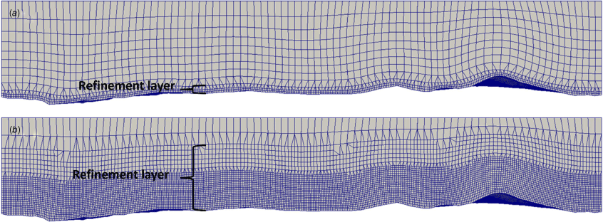
The WindNinja mesh is constructed to conform to the terrain and is refined near the ground to better resolve the large gradients expected there (Fig. A1). This region of cell refinement near the ground is referred to as the ‘refinement layer’. The Base Case uses the ‘fine’ mesh choice setting in WindNinja, which results in a near-ground horizontal and vertical cell resolution of 24 m and a refinement layer depth of 96 m. Mesh resolution is investigated by (1) increasing the resolution of the refinement layer to 6 m, and (2) increasing the depth of the refinement layer to 900 m.
Side view of the mesh for (a) the Base Case, and (b) the sensitivity case with a refinement layer depth of 900 m.
Simulations with the RNG k-epsilon model (S4 settings) compared best with observations and are presented in the main body of the paper. This determination was made based on overall error metrics for mean wind speed, mean wind direction and TKE (Table A2) as well as qualitative comparisons of the modelled flow field and observations, including lidar scans. Table A2 shows that the S5 settings had the best comparisons for mean wind speed; however, this configuration resulted in unrealistic flow separation as detailed below and so was not considered an improvement over the Base Case. It is widely accepted that the RNG k-epsilon model tends to outperform the standard k-epsilon model in domains with flow separation (Papageorgakis and Assanis 1999), so our determination is in line with previous findings. Results from simulations with Base Case, S1, S2, S3, S4 and S5 settings are summarised below.
| Variable | Metric | B | S1 | S2 | S3 | S4 | S5 | |
|---|---|---|---|---|---|---|---|---|
| Wind speed (m s−1) | RMSE | 1.15 | 1.08 | 1.01 | 1.29 | 0.94 | 0.63 | |
| MBE | −0.63 | −0.52 | −0.48 | −0.58 | −0.61 | 0.15 | ||
| MAPE | 29.6 | 27.2 | 29.8 | 32.2 | 29.3 | 18.1 | ||
| Wind direction (°) | RMSE | 31.3 | 32.8 | 19.8 | 37.8 | 22.1 | 67.2 | |
| MBE | −15.5 | −14.5 | −14.3 | −18.5 | −6.38 | 35.9 | ||
| MAPE | 12.2 | 12.8 | 11.4 | 14.8 | 8.37 | 22.9 | ||
| TKE (m2 s−1) | RMSE | 0.74 | 0.63 | 0.71 | 0.79 | 0.67 | 0.97 | |
| MBE | −0.37 | −0.26 | −0.35 | −0.51 | −0.25 | −0.44 | ||
| MAPE | 41.5 | 34.8 | 42.0 | 35.0 | 39.1 | 54.5 |
B is the Base case; S1 is the modified near-ground cell size case; S2 is the modified depth of refinement layer case; S3 is the modified roughness length case; S4 is the modified turbulence model case; S5 is the modified discretisation scheme case. The smallest value for each error metric is indicated in bold.
Near-ground cell size (S1)
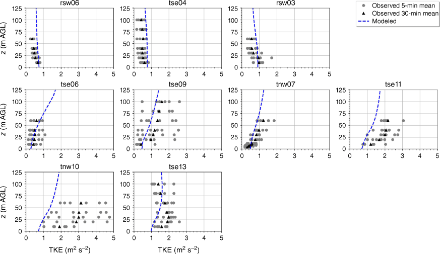
Increasing the near-ground horizontal and vertical cell size from 24 to 6 m does not appreciably change the key features in the modelled flow field (Fig. A2 vs Fig. A23). Some of the error metrics for mean wind slightly improve for this case (Table A2, Figs A3–A8).
Top view of the modelled flow field at (a) 40 m AGL, and (b) 100 m AGL for the modified near-ground cell size case.

Side view of the modelled flow field through (a) Transect A, and (b) Transect B for the modified near-ground cell size case. Tower labels indicate maximum sensor height for that tower.

Top view of the modelled TKE field at (a) 40 m AGL, and (b) 100 m AGL for the modified near-ground cell size case.

Side view of the modelled TKE field through (a) Transect A, and (b) Transect B for the modified near-ground cell size case. Tower labels indicate maximum sensor height for that tower.

Modelled vs observed mean wind speed at each tower for the modified near-ground cell size case. Grey circles indicate 5-min mean observations. Black triangles indicate 30-min mean observations. The top row of panels are the southwest ridge towers; the middle row of panels are the valley towers; the bottom row of panels are the northeast ridge towers.
Modelled vs observed mean wind direction at each tower for the modified near-ground cell size case. Grey circles indicate 5-min mean observations. Black triangles indicate 30-min mean observations. The top row of panels are the southwest ridge towers; the middle row of panels are the valley towers; the bottom row of panels are the northeast ridge towers.
Modelled vs observed mean TKE at each tower for the modified near-ground cell size case. Grey circles indicate 5-min mean observations. Black triangles indicate 30-min mean observations. The top row of panels are the southwest ridge towers; the middle row of panels are the valley towers; the bottom row of panels are the northeast ridge towers.
Increasing the depth of the refinement layer from 96 to 900 m does not appreciably change the key features in the modelled flow field (Fig. A9 vs Fig. A23). The increased refinement above 96 m does not appear to resolve additional features in the flow or TKE fields throughout the vertical profile (Figs A9 and A11 vs Figs A23 and A26). Some of the error metrics improve slightly for this case (Table A2, Figs A10, A12–A15).
Top view of the modelled flow field at (a) 40 m AGL, and (b) 100 m AGL for the modified refinement layer depth case.

Side view of the modelled flow field through (a) Transect A, and (b) Transect B for the modified refinement layer depth case. Tower labels indicate maximum sensor height for that tower.

Top view of the modelled TKE field at (a) 40 m AGL, and (b) 100 m AGL for the modified refinement layer depth case.

Side view of the modelled TKE field through (a) Transect A, and (b) Transect B for the modified refinement layer depth case. Tower labels indicate maximum sensor height for that tower.

Modelled vs observed mean wind speed at each tower for the modified refinement layer depth case. Grey circles indicate 5-min mean observations. Black triangles indicate 30-min mean observations. The top row of panels are the southwest ridge towers; the middle row of panels are the valley towers; the bottom row of panels are the northeast ridge towers.
Modelled vs observed mean wind direction at each tower for the modified refinement layer depth case. Grey circles indicate 5-min mean observations. Black triangles indicate 30-min mean observations. The top row of panels are the southwest ridge towers; the middle row of panels are the valley towers; the bottom row of panels are the northeast ridge towers.
Modelled vs observed mean TKE at each tower for the modified refinement layer depth case. Grey circles indicate 5-min mean observations. Black triangles indicate 30-min mean observations. The top row of panels are the southwest ridge towers; the middle row of panels are the valley towers; the bottom row of panels are the northeast ridge towers.
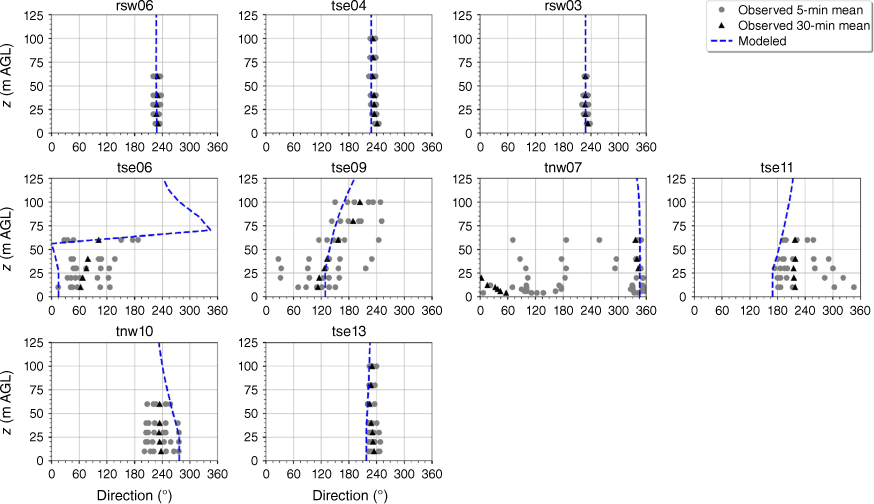
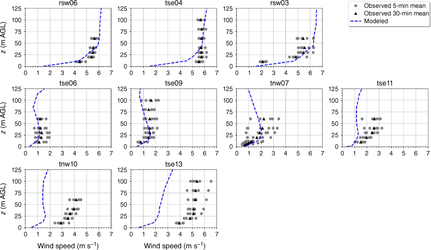
Decreasing the roughness length from 0.43 to 0.1 m does not appreciably change the key features in the modelled flow field (Fig. A16 vs Fig. A23). Some of the error metrics for mean wind slightly improve for this case (Table A2, Figs A17–A21).
Top view of the modelled flow field at (a) 40 m AGL, and (b) 100 m AGL for the modified roughness length case.

Side view of the modelled flow field through (a) Transect A, and (b) Transect B for the modified roughness length case. Tower labels indicate maximum sensor height for that tower.

Top view of the modelled TKE field at (a) 40 m AGL, and (b) 100 m AGL for the modified roughness length case.

Side view of the modelled TKE field through (a) Transect A, and (b) Transect B for the modified roughness length case. Tower labels indicate maximum sensor height for that tower.

Modelled vs observed mean wind speed at each tower for the modified roughness length case. Grey circles indicate 5-min mean observations. Black triangles indicate 30-min mean observations. The top row of panels are the southwest ridge towers; the middle row of panels are the valley towers; the bottom row of panels are the northeast ridge towers.
Modelled vs observed mean wind direction at each tower for the modified roughness length case. Grey circles indicate 5-min mean observations. Black triangles indicate 30-min mean observations. The top row of panels are the southwest ridge towers; the middle row of panels are the valley towers; the bottom row of panels are the northeast ridge towers.
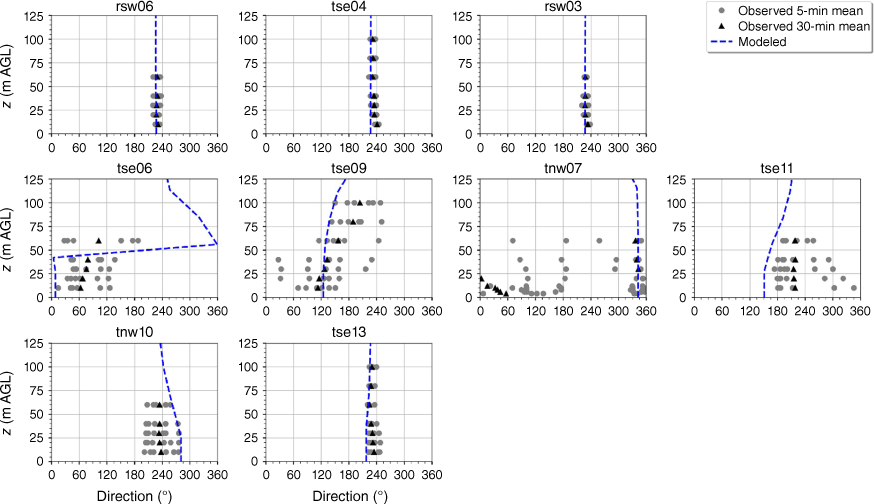
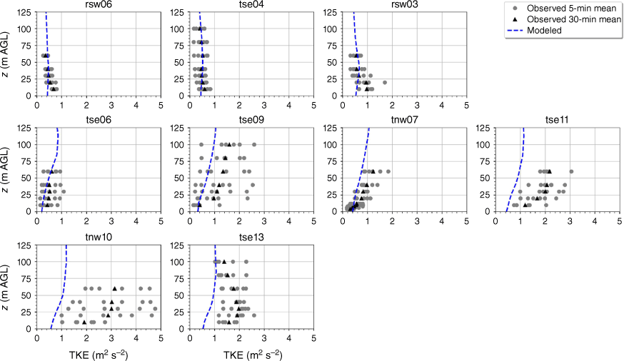
Changing the turbulence model from the k-epsilon model to the RNG k-epsilon model induces some notable changes in the flow field (Fig. 3 vs Fig. A23). The wake and recirculation regions are slightly smaller with the RNG k-epsilon model. Note how there is more speed-up along the second ridge between Transects A and B for this case than for the Base Case (Fig. 3 vs Fig. A22). The vertical slices show some differences in the vertical profiles of the flow and TKE fields as well (Figs 4 and 6 vs Figs A24 and A26). The recirculation zones shift downward slightly in both transects and you can see the stronger flow over the second ridge (Fig. 4 vs Fig. A24). The TKE values are slightly higher and the region of enhanced TKE penetrates further down into the valley (Fig. 8 vs Fig. A26). All of the error metrics improve for this case (Table A2, Figs A25, A27, A28).
Modelled vs observed mean TKE at each tower for the modified roughness length case. Grey circles indicate 5-min mean observations. Black triangles indicate 30-min mean observations. The top row of panels are the southwest ridge towers; the middle row of panels are the valley towers; the bottom row of panels are the northeast ridge towers.
Top view of the modelled flow field at (a) 40 m AGL, and (b) 100 m AGL for the Base Case (k-epsilon model).

Side view of the modelled flow field through (a) Transect A, and (b) Transect B for the Base Case (k-epsilon model). Tower labels indicate maximum sensor height for that tower.

Top view of the modelled TKE field at (a) 40 m AGL, and (b) 100 m AGL for the Base Case (k-epsilon model).

Side view of the modelled TKE field through (a) Transect A, and (b) Transect B for the Base Case (k-epsilon model). Tower labels indicate maximum sensor height for that tower.

Modelled vs observed mean wind speed at each tower for the Base Case (k-epsilon model). Grey circles indicate 5-min mean observations. Black triangles indicate 30-min mean observations. The top row of panels are the southwest ridge towers; the middle row of panels are the valley towers; the bottom row of panels are the northeast ridge towers.
Modelled vs observed mean wind direction at each tower for the Base Case (k-epsilon model). Grey circles indicate 5-min mean observations. Black triangles indicate 30-min mean observations. The top row of panels are the southwest ridge towers; the middle row of panels are the valley towers; the bottom row of panels are the northeast ridge towers.
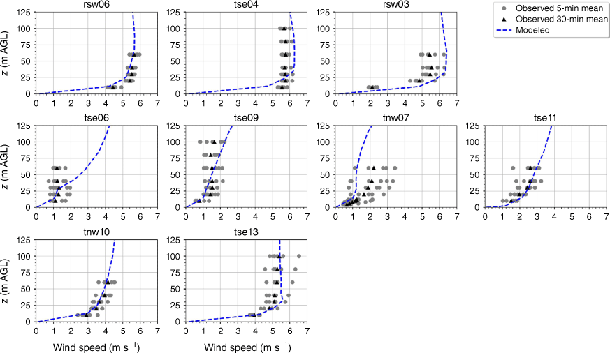
On visual inspection of the surface, slice and scatter plots, the change in the discretisation scheme induces the largest differences in the flow field. Notably, the QUICK scheme produces substantially shorter, narrower and shallower regions of flow separation and recirculation compared with the linear upwind scheme used in the Base Case (Fig. A29 vs Fig. A22). The mean wind speed predictions in the valley and on the second ridge improve slightly (Fig. A33 vs Fig. A26) and this results in an overall improvement in RMSE, MBE and MAPE in mean wind speed for this case. The improved mean wind speed predictions in the valley and on the second ridge are because the recirculation zone behind the first ridge shrinks substantially when QUICK is used instead of linear upwind (Fig. A29 vs Fig. A22 and Fig. A30 vs Fig. A23). In fact, there is no recirculation predicted along Transect B at all (Fig. A30). This does not match the sonic anemometer observations reported here or the lidar data reported in Menke et al. (2019). Menke et al. (2019) reported a well-defined recirculation zone along Transect B. The high temporal variability observed in the wind direction data (Fig. 11) further support the existence of a turbulent recirculation region along Transect B. For these reasons, we believe the QUICK discretisation scheme produces a less realistic flow field than the linear upwind scheme used in the base case (Figs A30, A31, A32, A34–A36).
Modelled vs observed mean TKE at each tower for the Base Case (k-epsilon model). Grey circles indicate 5-min mean observations. Black triangles indicate 30-min mean observations. The top row of panels are the southwest ridge towers; the middle row of panels are the valley towers; the bottom row of panels are the northeast ridge towers.
Top view of the modelled flow field at (a) 40 m AGL, and (b) 100 m AGL for the modified discretisation scheme case.

Side view of the modelled flow field through (a) Transect A, and (b) Transect B for the modified discretisation scheme case. Tower labels indicate maximum sensor height for that tower.

Top view of the modelled TKE field at (a) 40 m AGL, and (b) 100 m AGL for the modified discretisation scheme case.

Side view of the modelled TKE field through (a) Transect A, and (b) Transect B for the modified discretisation scheme case. Tower labels indicate maximum sensor height for that tower.

Modelled vs observed mean wind speed at each tower for the modified discretisation scheme case. Grey circles indicate 5-min mean observations. Black triangles indicate 30-min mean observations. The top row of panels are the southwest ridge towers; the middle row of panels are the valley towers; the bottom row of panels are the northeast ridge towers.
Modelled vs observed mean wind direction at each tower for the modified discretisation scheme case. Grey circles indicate 5-min mean observations. Black triangles indicate 30-min mean observations. The top row of panels are the southwest ridge towers; the middle row of panels are the valley towers; the bottom row of panels are the northeast ridge towers.
Modelled vs observed mean TKE at each tower for the modified discretisation scheme case. Grey circles indicate 5-min mean observations. Black triangles indicate 30-min mean observations. The top row of panels are the southwest ridge towers; the middle row of panels are the valley towers; the bottom row of panels are the northeast ridge towers.
