

Advancing spatial analysis of invasive species movement data to improve monitoring, control programs and decision making: feral cat home range as a case study
Cameron Wilson A B * , Matthew Gentle B C and Bronwyn Fancourt A B D
A
B
C
D
Abstract
Many invasive animals are typically active across large areas, making monitoring and control programs expensive. To be efficacious, monitoring devices and control tools need to be strategically located to maximise the probability of encounter. This requires an understanding of how the target species uses the landscape, through identifying key habitat or landscape features that are preferred and used disproportionately more frequently by the species. Spatial analysis of animal movements can help identify high use areas.
The variability introduced by different range calculation methods can lead to uncertainty in subsequent habitat analyses. We aimed to determine which method is superior for accurate delineation of core areas for feral cats.
We analysed spatial data from 35 collared feral cats across four Australian study sites between 2016 and 2019, and compared the core areas generated using seven commonly used home range estimation methods.
We found that the α-hull method provided a higher precision of polygon placement, resulting in lower Type I and II errors and higher conformity to landscape features than other methods. The α-hull used a single default parameter and required no subjective input, making it a more objective, superior method.
We recommend that the α-hull method be used to define core activity areas for feral cats, enabling more robust habitat analysis, and identification of key habitat and landscape features to strategically target for monitoring and control programs.
This strategic approach could significantly improve cost efficiencies, particularly where existing management is widely dispersed, and core activity areas are clumped.
Keywords: core area, Felis catus, feral cat, GPS collar, home range, kernel, LoCoH, MCP, α-hull.
Introduction
Invasive animals are a significant global threat to biodiversity (Doherty et al. 2016), primary production (Schley et al. 2008) and human health (Chinchio et al. 2020). Many invasive animals are active over large areas (e.g. feral pig), or else are solitary and elusive (e.g. feral cat). These challenges make monitoring and control programs resource hungry and if not planned well, ineffective. Density and abundance are often determined by the placement of monitoring devices at defined intervals (e.g. Allen et al. 2013) or else at random (e.g. Guerrasio et al. 2022). However, in these situations, target species detection is reliant upon random encounters with monitoring devices. Similarly, large numbers of poison baits are often scattered broadly with the intent to saturate the landscape to increase the likelihood of bait encounters (e.g. Fancourt et al. 2021). In Fancourt et al. (2021)’s case, bait placement along tracks proved insufficient to significantly reduce the feral cat population, highlighting that in such cases, an over-reliance upon random encounters is likely to be both ineffective and inefficient. This was not the case in Ballard et al. (2020), where landscape saturation of baits resulted in a 90% mortality rate in collared wild dogs. However, such saturation may also increase the likelihood of nontarget species mortality. As such, improving monitoring or control tool placement to target locations of likely higher use of the intended species (Harriott et al. 2021; Wilson et al. 2023a), is likely to improve encounter rates in monitoring and control programs, while simultaneously reducing the probability of nontarget encounters.
Home range areas are widely reported in invasive animal literature (Amos et al. 2014; McGregor et al. 2015; Wilson et al. 2023b) but have limited practical value for improving monitoring or control programs. Animal-borne global positioning system (GPS) units are often used to collect spatial information about an animal’s movements, with location fixes being recorded by the GPS at predetermined time intervals. An animal’s home range calculation typically encompasses 90–100% of the location fixes, but in doing so, it fails to identify key areas of higher use. Most animals do not use the landscape uniformly, but instead have core areas where they spend disproportionately more time. For example Edwards et al. (2001) demonstrated that 50% of feral cat location fixes could be found in just 25% of the cat’s home range area. By defining and interrogating these core areas, we can gain better insight into which features (e.g. vegetation, water, landscape features) are preferred by the target animal, allowing us to strategically focus our monitoring and control efforts into these preferred features across the landscape.
An animal’s core area is often defined as the area encompassing the densest 50% of location fixes (Getz et al. 2007). There are many range calculation methods available to analyse spatial data and discriminate these core areas that produce different area estimations for the same animal. For example, Molsher et al. (2005) found that the mean 95% minimum convex polygon (MCP) area was over 33% smaller than the mean 95% fixed kernel density estimate for the same group of feral cats. Several factors contribute to such differences in area estimation, with some methods being more sensitive to different factors than others. For example, it has been shown that excessive bandwidth of the hREF smoothing parameter overestimates home range size (Naef-Daenzer 1993; Seaman and Powell 1996) in comparison to least-squares cross validation (LSCV) and MCP. Notwithstanding, MCP bias increases with sample size (Burgman and Fox 2003) and is very sensitive to outlying points (Burgman and Fox 2003). By understanding how each of these calculation methods can be influenced by different variables in our data, we can identify which methods more accurately discriminate core areas for the target species, and therefore which method can be used to better inform future research into resource selection and consequently monitoring and control programs.
We used a feral cat GPS collar dataset collected from three geographically distinct areas in Queensland across four years, to estimate home range and core areas using seven commonly used estimation approaches. We compared activity range polygon construction across methods and evaluated each output to identify strengths and limitations for each method. We discuss our findings and make recommendations for the most appropriate method to define core areas to improve monitoring and control of feral cats.
Methods
Ethics approvals
This study was approved by the DAF Community Access Animal Ethics Committee (Permit CA 2016-02-946).
Study sites
We collected spatial data from GPS collars fitted to feral cats across three geographically distinct national parks in Queensland, Australia (Fig. 1) over four years (2016–2019) as part of a larger feral cat baiting efficacy study (Fancourt et al. 2021, 2022a, 2022b). Detailed site descriptions including location coordinates, bioregion, environ and dominant vegetation communities at each site are provided in Fancourt et al. (2022b).
Map showing the location of the three study sites used in the current study within Queensland. Insets on left show (a) Moorrinya National Park, (b) Taunton National Park (Scientific) and (c) Currawinya National Park. Inset at top right shows location of Queensland within Australia.
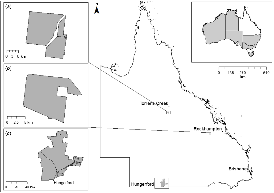
Taunton National Park (Scientific) (TNP) is located in the subtropical, Brigalow-belt region of central Queensland, approximately 150 km west of Rockhampton (Department of Environment and Resource Management 2011a). During the study period, rainfall at the site varied between years, with above average rainfall of 418 mm received during the five month study period in 2016, but below average rainfall of 88 mm received over the same period in 2017 (Bureau of Meteorology 2020a).
Currawinya National Park (CNP) is located in the semiarid region of south-west Queensland, approximately 25 km north-west of Hungerford. The site encompasses a range of different landscapes ranging from sand dunes and open plains to lakes, saltpans and riparian zones (Queensland Parks and Wildlife Service 2001). The study season was very dry and the site received just 11 mm of rainfall across the five month study period (Bureau of Meteorology 2020b).
Moorrinya National Park (MNP) is located 85 km south of Torrens Creek in the Desert Uplands region of central Queensland (Department of Environment and Resource Management 2011b). During the three-month study period, the study site received a slightly below average rainfall of 22 mm (Bureau of Meteorology 2020c).
Data collection
Between 2016 and 2019, we captured 56 feral cats (36 male, 20 female) using a mix of cage traps and padded soft-jaw foothold traps lured with a range of food and scent lures, as described in Fancourt et al. (2021) and Fancourt et al. (2022a). Captured cats were sedated and fitted with Quantum 4000E (Telemetry Solutions, Concord, California, United States) collars equipped with both VHF and GPS capabilities (see detailed methods in Fancourt et al. (2021)). To reduce autocorrelation of data points, GPS collars were programmed to take location fixes every 12 h (at 10:00 hours and 22:00 hours daily). Cat movements were recorded continuously for between 10 and 155 days. Detailed information for all 56 cats are listed in Supplementary Table S1. Of the 56 cats collared, 35 cats (24 male, 11 female) provided adequate data (>40 days as per Leo et al. (2016)) for further analysis. The number of collared cats per site, number of days collared and date ranges of GPS data for these 35 cats are presented in Table 1.
| Site | Year | No. of cats collared | No. of cats used for analysis | No. of days GPS data | Date range | ||||
|---|---|---|---|---|---|---|---|---|---|
| M | F | M | F | Mean | Range | ||||
| TNP | 2016 | 6 | 4 | 5 | 4 | 88 | 20–155 | May–September (1 cat to October) | |
| TNP | 2017 | 10 | 5 | 7 | 3 | 69 | 19–112 | May–September | |
| CNP | 2018 | 11 | 6 | 5 | 3 | 67 | 10–143 | April–September | |
| MNP | 2019 | 9 | 5 | 7 | 1 | 57 | 34–130 | July–September (1 cat to December) | |
| Total | 36 | 20 | 24 | 11 | |||||
For details of individual cats, see Table S1.
M, male; F, female; TNP, Taunton National Park; CNP, Currawinya National Park; MNP, Moorrinya National Park.
GPS collar positional accuracy test
We used the test collar data collected by Fancourt et al. (2021) to determine the most appropriate criteria for identifying and removing inaccurate and imprecise points from our dataset. We investigated precision of points with horizontal dilution of precision (HDOP) values ranging between 3 and 9 and number of satellites between 2 and 3. These test data were collected using the same GPS collar make and model fitted to the cats in the current study. However, as we were not investigating fine scale cat movements, we adopted a coarser resolution (i.e. fix >50 m away from the true position) than adopted by Fancourt et al. (2021) to classify a fix as imprecise.
Data clean-up
GPS collar data collected in the current study were truncated to retain only those fixes commencing 24 h after collaring (to allow the sedative drugs used during collaring to wear off and the cat to resume normal activity) and up to the known date of death (e.g. shot, see Table S1). For cats that were not shot, an estimated date of death was recorded, as determined by the cat’s final fix location before obvious movements ceased. All remaining fixes were reviewed to identify and remove any potentially imprecise fixes and GPS measurement errors following the three-step process outlined in Fancourt et al. (2021). First, all attempted fixes that did not successfully record a northing coordinate were classified as a ‘failed fix’ and removed from the dataset. Second, all remaining fixes that met the criteria for ‘imprecise’ (based on the GPS collar positional accuracy test) were identified and removed. Third, the remaining fixes were loaded into ArcMap® and visually inspected to identify and remove any obvious outliers (i.e. fixes located in impossible to reach locations, such as the ocean).
Home range and core area estimations
We quantified the home range and core area using the 90% and 50% isopleths, respectively. We adopted these isopleths as Börger et al. (2006) has demonstrated reduced accuracy using isopleths above 90% and below 50%. All calculations were performed using the adehabitatHR package 0.4.16 (Calenge 2006) in R ver. 3.6.2 (R Core Team 2019). Maps showing location fixes, 90% home range and 50% core area isopleths were generated using ArcMap® ver. 10.7.1 (ESRI 2019). Details of the seven estimation methods used to quantify home range and core area for each cat are outlined below:
Minimum Convex Polygon – all default values used.
Fixed Kernel Density Estimates – we used the two most common smoothing parameters: reference value (hREF) and least-squares crossvalidation (LSCV), to quantify fixed kernel density estimates. The default value of both parameters was used to avoid subjectivity. The smallest grid size (100 pixels) and the default resolution (extent) were used, as recommended by Seaman and Powell (1996).
Local Convex Hull – we estimated home range and core areas using all three local convex hull methods; nearest neighbour (k), fixed sphere-of-influence (r) and adaptive (a) (as described in Getz et al. (2007)), using the following relative parameters:
K = √n, where n = sample size
r = half the maximum nearest-neighbour distance
a = maximum distance between any two points.
The k parameter was determined by implementing the formula suggested by Getz et al. (2007). To calculate the r and a parameters, the dataset was loaded into ArcMap® and the maximum nearest-neighbour and maximum distance between any two points was measured. Individual parameter values were calculated for each individual cat. An average value across all cats was not considered representative, given large variations in point distribution across years, study sites, sex, age and habitats. Although the minimum spurious hole covering (MSHC) method can account for large physical and inhospitable landscape features that cannot be used by the study animal, such as lakes, shorelines, cliffs, etc. (Getz and Wilmers 2004), such obvious features were not present at our study sites during the study period, and so the MSHC rule was not adopted in our calculations.
Alpha-hull (α-hull) – we used the CharHull method as described in Calenge (2011), adopting the default alpha (α) value to avoid the potential for bias and to facilitate comparisons with other studies.
Comparison of home range (90% isopleth) and core area (50% isopleth) estimations
The relationship between home range size and core area size was determined by taking the mean proportions of core area to home range for each cat, with both sexes and all sites combined.
Comparison and evaluation of core area polygon construction
The estimated core area and the corresponding polygon construction were evaluated for efficiency and effectiveness by interrogating outputs for: (1) area estimation variability across methods; (2) Type I errors (excluded points) and Type II errors (unused area included within the polygon); (3) the influence of parameter values; (4) consistency across nonuniform datasets and distributions; and (5) landscape feature conformity.
Results
GPS collar positional accuracy test
Fancourt et al. (2021) recorded 396 attempted positional fixes across three test locations, including 46 failed fixes. Of the 350 successful fixes, a further 46 were considered imprecise for our study (>50 m away from the true collar position). The number of satellites used for each fix was the largest contributor to positional error, with 43 of the 46 (93%) imprecise fixes only securing ≤3 satellites to record the collar position. By removing all fixes with ≤3 satellites from the dataset, 32 of the 304 precise fixes (11%) would also be removed (Table S2), reducing the number of fixes retained for subsequent analyses. However, the loss of some accurate fixes was considered necessary to ensure as many imprecise fixes were removed from the dataset as possible, thereby maximising the precision of points in the retained dataset.
Data clean-up
Results of the data clean-up process for each dataset are displayed in Table 2.
| TNP 2016 | TNP 2017 | CNP 2018 | MNP 2019 | ||
|---|---|---|---|---|---|
| Attempted fixes | 1565 | 1776 | 1568 | 1054 | |
| Remove: fixes outside of truncated date range | 19 | 158 | 20 | 11 | |
| Remove: failed fix attempts | 51 | 66 | 178 | 0 | |
| Remove: imprecise fixes using ≤3 satellites | 102 | 123 | 28 | 221 | |
| Remove: impossible outliers | 0 | 1 | 29 | 1 | |
| Total fixes removed | 172 | 348 | 255 | 233 | |
| Total fixes retained (no.) | 1393 | 1428 | 1313 | 821 | |
| Total fixes retained (%) | 89 | 80 | 84 | 78 | |
| No of collared cats | 9 | 10 | 8 | 8 | |
| No of fixes retained per cat: | |||||
| Mean | 155 | 143 | 164 | 132 | |
| Range | 129–208 | 70–220 | 81–221 | 81–177 |
TNP, Taunton National Park; CNP, Currawinya National Park; MNP, Moorrinya National Park.
Home range estimations (90% isopleth)
Mean home range estimates for each method are shown in Table 3. Individual estimates for each cat are presented in Table S3. As data were only available for one female cat at MNP, this data source was excluded from further analyses. Across TNP and CNP, the mean home range size for male cats was consistently larger than the corresponding female home range size for each of the seven estimation methods, with only one exception (r-LoCoH at CNP). For all years and sites combined, female ranges approximated between 38 and 74% of the size of male home ranges. Female cats at CNP had larger home ranges than both TNP years for all estimation methods. With the exception of male kernel (LSCV) ranges, all methods across both sexes demonstrated smaller ranges at TNP in 2017 than 2016. Besides this, there was no clear effect of site on male home ranges, with estimation method influencing the result.
| Sex | Method | TNP 2016 (km2) | TNP 2017 (km2) | CNP 2018 (km2) | MNP 2019 (km2) | |
|---|---|---|---|---|---|---|
| Male | Sample size | n = 5 | n = 7 | n = 5 | n = 7 | |
| Kernel (hREF) | 49.0 ± 66.2 | 18.2 ± 12.0 | 48.2 ± 22.3 | 18.6 ± 4.7 | ||
| Kernel (LSCV) | 6.5 ± 7.9 | 7.4 ± 6.6 | 8.0 ± 5.7 | 5.9 ± 5.3 | ||
| MCP | 27.3 ± 35.0 | 11.2 ± 7.7 | 24.6 ± 9.6 | 10.9 ± 3.5 | ||
| a-LoCoH | 12.3 ± 13.6 | 5.7 ± 3.5 | 12.6 ± 4.7 | 6.5 ± 2.5 | ||
| r-LoCoH | 8.5 ± 9.5 | 2.8 ± 1.4 | 3.8 ± 2.5 | 3.4 ± 2.1 | ||
| k-LoCoH | 8.9 ± 8.3 | 4.7 ± 3.1 | 8.3 ± 3.8 | 5.8 ± 1.9 | ||
| α-hull | 15.9 ± 13.4 | 8.7 ± 6.9 | 20.5 ± 8.9 | 10.8 ± 4.0 | ||
| Female | Sample size | n = 4 | n = 3 | n = 3 | n = 1 | |
| Kernel (hREF) | 16.1 ± 9.7 | 4.4 ± 3.0 | 31.6 ± 12.4 | 24.2 | ||
| Kernel (LSCV) | 2.7 ± 1.7 | 1.9 ± 2.1 | 3.4 ± 2.7 | 2.1 | ||
| MCP | 9.2 ± 5.5 | 2.5 ± 1.7 | 19.2 ± 4.8 | 9.6 | ||
| a-LoCoH | 4.4 ± 2.2 | 1.5 ± 1.4 | 10.6 ± 5.9 | 8.5 | ||
| r-LoCoH | 1.5 ± 1.1 | 0.4 ± 0.3 | 8.6 ± 7.7 | 2.4 | ||
| k-LoCoH | 3.5 ± 1.9 | 1.4 ± 1.3 | 7.7 ± 4.3 | 8.4 | ||
| α-hull | 6.2 ± 1.6 | 1.8 ± 1.5 | 13.9 ± 6.7 | 11.3 |
TNP, Taunton National Park; CNP, Currawinya National Park; MNP, Moorrinya National Park; a-LoCoH, adaptive local convex hull; r-LoCoH, fixed-sphere-of-influence local convex hull; k-LoCoH, nearest-neighbour local convex hull.
Core area estimations (50% isopleth)
Mean core area estimates for each method are shown in Table 4. Individual estimates for each cat are presented in Table S4. As data were only available for one female cat at MNP, this data source was excluded from further analyses. Male cats demonstrated larger core areas than females for all range calculation methods at TNP (both years), with female ranges between 24 and 44% of the size of male ranges. CNP demonstrated slightly different results according to calculation method, with r-LoCoH, k-LoCoH and α-hull all demonstrating larger female core areas than males. With the exception of kernel (LSCV), female cats at CNP demonstrated larger core areas than both TNP years. As with the home range estimations, TNP 2017 ranges were typically smaller than 2016 ranges, with the exception of male kernel (LSCV) and α-hulls. There was no clear effect of site on male core area, with estimation method influencing the result.
| Sex | Method | TNP 2016 (km2) | TNP 2017 (km2) | CNP 2018 (km2) | MNP 2019 (km2) | |
|---|---|---|---|---|---|---|
| Male | Sample size | n = 5 | n = 7 | n = 5 | n = 7 | |
| Kernel (hREF) | 13.0 ± 16.2 | 5.8 ± 4.4 | 14.0 ± 7.4 | 5.2 ± 2.2 | ||
| Kernel (LSCV) | 0.7 ± 0.8 | 1.7 ± 2.0 | 0.4 ± 0.3 | 1.3 ± 1.8 | ||
| MCP | 8.5 ± 9.7 | 4.1 ± 3.0 | 9.5 ± 6.0 | 3.2 ± 2.0 | ||
| a-LoCoH | 2.6 ± 2.3 | 1.8 ± 1.4 | 3.1 ± 1.7 | 1.8 ± 1.2 | ||
| r-LoCoH | 3.1 ± 3.2 | 1.2 ± 0.6 | 1.6 ± 0.8 | 1.5 ± 0.8 | ||
| k-LoCoH | 1.1 ± 1.0 | 1.1 ± 0.8 | 0.9 ± 0.7 | 1.1 ± 0.7 | ||
| α-hull | 1.0 ± 0.9 | 1.1 ± 0.9 | 0.8 ± 0.7 | 1.2 ± 0.7 | ||
| Female | Sample size | n = 4 | n = 3 | n = 3 | n = 1 | |
| Kernel (hREF) | 4.6 ± 3.1 | 1.4 ± 1.1 | 8.8 ± 4.5 | 5.0 | ||
| Kernel (LSCV) | 0.5 ± 0.4 | 0.5 ± 0.7 | 0.4 ± 0.3 | 0.3 | ||
| MCP | 3.9 ± 3.3 | 0.8 ± 0.6 | 4.9 ± 2.9 | 2.5 | ||
| a-LoCoH | 0.9 ± 0.5 | 0.6 ± 0.5 | 2.5 ± 1.7 | 1.5 | ||
| r-LoCoH | 0.7 ± 0.2 | 0.2 ± 0.2 | 4.5 ± 4.5 | 1.4 | ||
| k-LoCoH | 0.5 ± 0.3 | 0.4 ± 0.4 | 1.0 ± 0.4 | 0.5 | ||
| α-hull | 0.5 ± 0.2 | 0.3 ± 0.3 | 1.1 ± 0.9 | 0.8 |
TNP, Taunton National Park; CNP, Currawinya National Park; MNP, Moorrinya National Park; a-LoCoH, adaptive local convex hull; r-LoCoH, fixed-sphere-of-influence local convex hull; k-LoCoH, nearest-neighbour local convex hull.
Comparison of home range (90% isopleth) and core area (50% isopleth) estimations
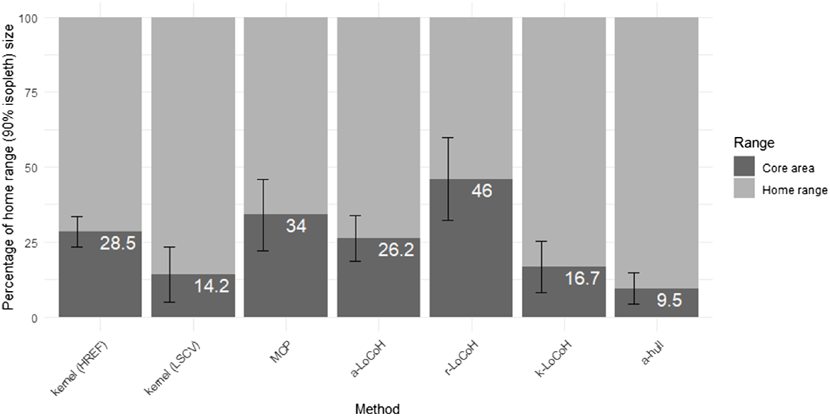
Despite the core area containing 50% of fixes, each method estimated a core area that was disproportionally smaller than the corresponding home range estimate (see Fig. 2). R-LoCoH demonstrated the largest proportional core area at 46% of the home range size, whereas the α-hull demonstrated the smallest proportional core area at just 9.5% of the corresponding home range size.
Mean proportional differences between home range (90% isopleth) and core area (50% isopleth) estimations for all cats in this study across all seven calculation methods. The white text on bars indicates the percentage of the home range that the core area encompasses. Error bars indicate standard deviation.
Comparison and evaluation of core area polygon construction
Proportional differences in core area between methods are shown in Table 5. Across all cats, the kernel (hREF) method demonstrated the largest mean core area of all methods examined. MCP method produced the second largest core area estimate, at 66% of the size of the kernel (hREF). The a-LoCoH was considerably smaller than either kernel (hREF) or MCP and on average, yielded estimates similar to those derived using r-LoCoH. Both r-LoCoH and a-LoCoH estimates were approximately twice as large as the α-hull, k-LoCoH and kernel (LSCV) estimates. The smallest core area estimations (α-hull, k-LoCoH and kernel (LSCV)) were just 12% the size of the kernel (hREF).
| Method | Kernel (hREF) | MCP | a-LoCoH | r-LoCoH | α-hull | k-LoCoH | |
|---|---|---|---|---|---|---|---|
| MCP | 0.66 | ||||||
| a-LoCoH | 0.26 | 0.39 | |||||
| r-LoCoH | 0.22 | 0.34 | 0.87 | ||||
| α-hull | 0.12 | 0.18 | 0.47 | 0.54 | |||
| k-LoCoH | 0.12 | 0.18 | 0.46 | 0.53 | 0.98 | ||
| Kernel (LSCV) | 0.12 | 0.18 | 0.46 | 0.53 | 0.98 | 1 |
The majority of cats (69%) demonstrated multiple discrete areas of high activity within their core area, represented by dense clusters of points. Because the MCP is unable to split polygons, it failed to distinguish these high use areas effectively, typically excluding all or part of a dense cluster of points (Type I error) while simultaneously including large unused areas (Type II error) (Fig. S1A). All other estimation methods were able to split the core area into discrete polygons (Fig. S1B–F) and thus outperformed the MCP when individuals displayed multiple discrete areas of high use. The r-LoCoH occasionally excluded some dense clusters (Fig. S1F), but this was not as pronounced as the MCP, nor did it occur for every cat. The inclusion of Type II errors in r-LoCoH was more extreme than in other hull methods (Fig. S1D, E, G), despite covering (on average) a similar core area to a-LoCoH (Table 5). The k-LoCoH method connected to distant, solitary points less frequently than other methods, often yielding the smallest core area (Table S4). The α-hull was the most efficient at constructing core area polygons, always including dense clusters (Fig. S1G). Despite often connecting dense clusters to distant points, the Delauney triangulation of the α-hull method created very thin polygons between distant points, minimising any exaggeration of the estimated core area and reducing Type II error. The kernel (LSCV) method occasionally demonstrated Type I errors when a grid intersection (used to estimate density – see Seaman and Powell (1996)) fell within a reasonably close group of points (e.g. Fig. S2), occasionally excluding valid points and simultaneously including unused area. This occurred for 11 cats (31%) and appeared to be more prevalent in those cats displaying high numbers of fixes. The smoothing parameter of the kernel (hREF) forced this method to include vast unused areas into the estimation (Type II error), thus inflating the size of the core area and generating the largest area estimation of all methods (Table 4).
Where the parameter was suboptimal in LoCoH methods, the size of the core area was sometimes overinflated due to an increase in the connection to distant, solitary points (Type II error). This appeared to be more exaggerated in a-LoCoH and r-LoCoH estimates than in k-LoCoH estimates across all data distribution types (i.e. large/small sample size; clustered/scattered distribution of fix locations) but particularly when there were fewer data points (Fig. S3A–C), resulting in much larger area estimations (Table 4). All cats in this study demonstrated fewer Type II errors in k-LoCoH than in a-LoCoH and r-LoCoH estimates, which suggests that at datasets of this size, the heuristic value for k is closer to the optimal than is the heuristic value for a and r. Although it is impossible to confirm the true optimal parameter value for real ecological data, core area estimations that demonstrate large Type II errors (Fig. S3B, C) suggest that their parameter is farther from the optimal. The minimum spurious hole-covering (MSHC) method could be implemented in this situation (Getz and Wilmers 2004), but this technique can be subjective. The greatest consistency was seen with the α-hull method, where the default value (α = 3 as per Calenge (2006)) was used across the entire dataset. This allowed for a more objective and comparable analysis across cats, given fewer and more consistent variables. The use of the default parameter for α-hull estimations resulted in core area polygons with minimal error and increased consistency across all data distribution types observed in this study. This simplicity and objectivity was not seen in kernel methods, where both kernel (LSCV) and (hREF) were influenced by three parameters: a smoothing parameter, grid size, and grid resolution (Seaman and Powell 1996). The default smoothing parameter in kernel (hREF) produces very large area estimations but the impact of grid size and resolution was not as evident in kernel (hREF) as it was in kernel (LSCV) due to the excessive influence of the smoothing parameter. The default smoothing parameter used in kernel (LSCV) estimations resulted in smaller and more distinct polygons depicting the core area in a more refined manner, however, it was more susceptible to influence by grid size and resolution, due to the reduced width of the smoothing parameter (Supplementary Material 4). Tweaking all three parameters to achieve the best outcome for each individual cat was exceptionally time-consuming, introduced the potential for bias, and increased the number of variables that had to be considered when comparing individuals.
The influence of nonuniform data distributions and sampling intensities on the output of the estimation varied depending on the method used. Where sample size was large, and the distribution of points was spatially scattered with few clusters (i.e. not concentrated along landscape features), the MCP and both kernel methods appear to do a reasonable job of estimating the core area (Fig. S5A, B and S6A). However, this combination of a large sample size and an even distribution was observed in less than 6% of cats. Where sample size was large but data demonstrated a clustered distribution, the MCP displayed both Type I and Type II errors (Fig. S1A) and the kernel (hREF) displayed very high Type II errors (Fig. S1B). In this situation, the kernel (LSCV) method would occasionally create a core area polygon with very high Type I errors (Fig. S4.1A). Small sample size and scattered data distribution forced the MCP and both kernel methods to include large Type II errors (Fig. S6B (kernel (LSCV)) and Fig. S7A, B (MCP and kernel (hREF))). LoCoH and α-hull appeared to produce more consistent core area estimates across different data distribution types than the MCP and kernel methods, and placed polygons with more precision, clearly highlighting the densest activity areas (Fig. S1D–G and S5C-D). Due to high variability with r-LoCoH, it sometimes produced a reasonably accurate core area estimation, despite a small sample size (Fig. S7C) but most of the time (74%) it produced an estimate considerably larger than other LoCoH methods (Fig. S8C), regardless of the data distribution. Of the three LoCoH methods, the k-LoCoH produced a smaller and more precise estimation than the other LoCoH methods across the following data distribution types: high n, clustered (Figs A1D and A9A); high n, scattered (Fig. S5C) and low n, scattered. The α-hull appeared to be marginally better than k-LoCoH at producing refined polygons with the inclusion of only small amounts of vacant land (Type II error) when the distribution had a high n and was clustered (Fig. S9B) but was comparable with other distribution types (Fig. S5).
The majority of cats (69%) in this study exhibited either tight clusters of GPS points or aligned their points with landscape features like creek lines. However, both the MCP and kernel (hREF) methods performed poorly in accurately representing landscape feature conformity for such distributions. This was mainly due to issues related to Type I and II errors and, for kernel (hREF), the influence of the smoothing parameter. The kernel (LSCV) method appeared to struggle to draw appropriate polygons when the dataset followed linear landscape features (e.g. creek, road), often placing polygons between points rather than over the top of the core clusters (Fig. S2), though it outperformed MCP and kernel (hREF) estimates where point distribution was not linear. The k-LoCoH appeared to conform well to landscape features, either when the distribution of points followed linear (Fig. S9A) or irregular features (Fig. S3A). Almost all cats at CNP demonstrated high activity concentrated along creek lines, and the k-LoCoH discerned these areas well. The a-LoCoH and r-LoCoH methods connected to more distant solitary points than k-LoCoH, therefore failing to produce a polygon with a commensurate degree of conformity to landscape features. Because of the sharp distinction of the core area polygons, the α-hull method also did well at defining the shape of landscape features that were of high use (Fig. S9B). Much like the k-LoCoH, α-hull ranges appeared to conform well, regardless of the distribution of points.
Discussion
We compared and contrasted the reliability and suitability of seven home range calculation methods to robustly describe core areas for feral cats. The choice of method had a strong influence on the size and accuracy of the core area (50%) estimation and any comparisons made thereafter. Five of the seven methods were plagued by high variability, high error rates, inconsistency across nonuniform datasets and irregular distributions resulting in inappropriate polygon placement and potential over/under exaggeration of core area estimations. The k-LoCoH and the α-hull appeared superior to the other methods due to their ability to overcome variations in data distribution and sample size, resulting in consistent, sharply defined polygons. However, the generally higher precision of the 50% polygon placement, resulting in lower Type I error inclusion, more definite landscape feature conformity and a uniform parameter value (α) suggested that the α-hull was preferable to k-LoCoH. Our findings suggest that the α-hull method is the most suitable choice for determining high activity areas for feral cats, facilitating more robust habitat analyses. Enhancing the cost effectiveness and efficacy of monitoring and control programs could be achieved by identifying preferred vegetation or landscape features of feral cats and strategically placing monitoring and control devices in these locations.
This study supports previous research indicating that male cats typically exhibit larger home ranges compared to females (Liberg et al. 2000; McGregor et al. 2015; Bengsen et al. 2016). However, there was an isolated exception observed at CNP, where the estimation of one female cat (2018_Cat04, as seen in Table S3) significantly amplified the mean differences of r-LoCoH range size between males and females. This exaggeration in results was unique to the r-LoCoH and highlights this methods’ inherent variability. The generally larger size of female ranges at CNP (most arid site) aligns with landscape productivity assessments reported by Bengsen et al. (2016). Likewise, the generally smaller range estimations at TNP in 2017–2016, reflect higher productivity during 2017, attributed to high rainfall prior to the study period, due to Cyclone Debbie.
Our findings are consistent with other studies (Konecny 1987; Edwards et al. 2001) that cats have multiple core areas, particularly in drier regions where the spatial separation of waterholes drives separation of prey, shelter and breeding females. In our study, male cats at the driest site (CNP) demonstrated the largest MCP, kernel (hREF) and a-LoCoH core area estimations across all study sites. In contradiction, male cats at CNP also demonstrated the smallest k-LoCoH, α-hull and kernel (LSCV) estimations across all study sites. The sensitivity of the MCP and kernel (hREF) to satellite data clusters (Burgman and Fox 2003) can lead to greatly exaggerated and inaccurate core area estimations (e.g. MCP – Fig. S1A), so the use of these methods for species exhibiting this type of activity is not advised. The smaller and more refined nature of polygons created by hull methods and the kernel (LSCV) demonstrated greater precision in the differentiation between high and low use areas, even when they were greatly dispersed, demonstrating greater accuracy in core area estimations. The use of fixed time interval programming in collars, causing GPS recordings to occur at the same time each day, may result in misleading or biased data clusters due to the capture of repetitive behaviours associated with the time of day/night. To mitigate this potential bias, a rolling fix interval of 11 or 13 h, instead of 12-h intervals, would ensure that fixes are recorded at different times each day. However, repetitive behaviour patterns can also indicate the utilisation of specific landscape features, which can provide valuable insights for management purposes (Bracis et al. 2018; Campbell et al. 2021; Wilson et al. 2023a).
The influence of subjective input through parameter manipulation was of concern for some methods, where parameter selection greatly affected the occurrence of Type I and II errors. The introduction of these error types primarily stems from three factors: inappropriate polygon placement, parameter influence, and nonuniform datasets or distributions. These error types are often negatively associated, where the avoidance of one can lead to an increase in the other. However, minimising both error types is crucial for accurately depicting high activity areas. Kernel methods, which rely on three parameters, present a considerably higher risk of subjective input and error. Grid intersections in kernel methods can be adjusted by modifying the grid size and resolution (extent), whereas the degree of overlap between kernels at the intersections can be altered by changing the smoothing parameter. The default smoothing parameter in kernel (hREF) is larger than in kernel (LSCV), resulting in area estimations and polygons that are excessively large for accurately representing the core area and the fine-scale habitat use analysis required (Calenge 2006). Refining all three parameters described above to achieve optimal outcomes for each individual cat is exceptionally time-consuming and increases the number of variables that need to be considered during data analyses. Our results demonstrate that r-LoCoH, which readily portrays high error levels, is somewhat erratic and therefore the least reliable LoCoH method, consistent with the findings of Getz et al. (2007). But Getz et al. (2007) also suggest that a-LoCoH outperforms both r-LoCoH and k-LoCoH due to its heuristic parameter being closer to the optimal value across a wider range of datasets. Because we used real ecological data in this study, we cannot know for certain what the optimal value for any of the LoCoH methods were, and it is difficult to draw conclusions from the data without any level of subjectivity. However, given the optimal LoCoH parameter is defined as the value that minimises the total error for the corresponding method (Getz et al. 2007), it is apparent that the heuristic k value for k-LoCoH is closer to the optimal value than for other LoCoH methods due to substantially fewer Type I and II errors at the sample sizes used in this study. Furthermore, employing a single parameter value derived from a mathematical formula like k-LoCoH reduces the risk of subjective input. In contrast to Bengsen et al. (2012), we did not utilise averaged LoCoH parameter values across all cats due to substantial variations in the dataset between individuals and study sites, leading to average parameters that yielded larger and more frequent errors. Additionally, we did not employ the Minimum Spurious Hole Covering (MSHC) rule (Getz and Wilmers 2004), as this technique can be less effective in landscapes with few inhospitable features, as observed in our study sites, and can therefore introduce a significant level of subjective input. The α-hull avoids subjective input by using a default, uniform parameter (α) across the entire dataset, making it a preferable choice over most other methods examined in this study.
The influence of inconsistency in sample size and data distributions (scattered vs clustered) varied according to method. For instance, kernel methods do not converge on the true extent of a home range as sample size increases (Seaman et al. 1999; Getz and Wilmers 2004). These methods also demonstrate higher error rates under such circumstances (Naef-Daenzer 1993; Worton 1995). Our findings of large sample sizes with clustered distributions (Fig. S4.1A) support this hypothesis. However, it is inappropriate to infer that kernels will perform well at small sample sizes, as the increased likelihood of a scattered distribution is likely to yield large Type II errors (see Figs S7B for kernel (hREF) and S6B for kernel (LSCV)). In practical scenarios, such as this, we cannot know for certain that the cat did not use areas we consider as Type II errors, and lower sample sizes may be the cause of the scattered distributions, rather than the habits of the cat or the nature of the landscape. But it was evident that low sample size with scattered distributions greatly inflate kernel core area size. Autocorrelated kernel density estimate (aKDE) home ranges have been demonstrated to perform well in these scenarios (Fleming et al. 2015). However, because previous studies on feral cat ranges have predominantly focused on kernel (hREF) methods (Table S5), and aKDE core ranges in our study were nearly identical to kernel (hREF) (Supplementary Fig. S10), we excluded aKDE from further analysis. Datasets with high sample size and scattered distributions may allow for reasonable MCP core area estimations (Fig. S5A) but this deteriorates rapidly when the distribution becomes clustered (Fig. S1A) or scattered with low sample sizes (Fig. S7A). The high variability demonstrated by the MCP and both kernel methods do not promote confidence in their use for core range estimations (Table S5).
The high variability in core area estimations observed with r-LoCoH was consistent with findings by Getz et al. (2007), although the source of variability was unconfirmed. The ability of the remaining hull methods to produce consistent core area estimation across multiple data distribution types seen in this study (high sample size and clustered; high sample size and scattered; and low sample size and scattered) further demonstrates their superiority over kernel methods, the MCP and r-LoCoH. In our view, opting for a-LoCoH instead of k-LoCoH or α-hull, as observed in Bengsen et al. (2012) and Recio and Seddon (2013), likely results in exaggerated estimations of core area size. The k-LoCoH and α-hull produced estimations that were smaller and more precise across all distribution types seen in this study. However, the α-hull demonstrates lower Type II error when applied to datasets with high sample size and clustered distributions (Fig. S8D) and demonstrates a finer conformity to landscape features (Fig. S9B). Burgman and Fox (2003) state that the α-hull converges on the true distribution with higher sample sizes, but we found that it performed remarkably well across all data distribution types observed in this study.
Our research suggests that the α-hull method is superior for accurately delineating core areas for feral cats. The α-hull’s strength lies in its high precision of polygon placement, low Type I and II errors, strong conformity to landscape features, repeatability and avoidance of subjective input. On average, α-hull core areas demonstrated the smallest comparative size (i.e. 9.5%, see Fig. 2) to corresponding home ranges of all methods studied here. This generates confidence in estimates of core area placements, which in turn instils confidence in subsequent assessments of habitat preference. If the MSHC rule is not applied to the LoCoH estimations, the default α value by adehabitatHR’s CharHull method (Calenge 2011) is more consistently accurate than the LoCoH heuristic values, introduces less potential bias, and is easier to implement. However, due to the process of polygon construction, the α-hull requires considerably longer computing time than other methods studied here. Nevertheless, the utilisation of the α-hull method provides representative information for subsequent analysis of critical habitat types and landscape features selected by cats in these core areas.
There are additional important considerations that may influence the outcomes of home range estimation. Autocorrelation is believed to influence the estimation of range distributions (Swihart and Slade 1985). To reduce such influence, previous feral cat studies have relied upon subsampling of data or low frequency location fixes (Table S5). Accordingly, we restricted location fixes to twice daily to reduce the effects of autocorrelation on estimates, although some likely remain. Methods that account for autocorrelation may permit a higher frequency of fixes to be included in analyses, although the impact on home range estimation in this study is likely to be minimal (Supplementary Material 10). We concur with Noonan et al. (2019) that developing estimators that account for autocorrelation with the precision of polygon placement of such methods such as LoCoH’s or α-hulls, would be highly beneficial. Additionally, temporal variability may influence the results of this study. Cats may alter their space use over time, likely in response to resource abundance, which may affect the outcomes of such studies.
The effectiveness of current control strategies is dependent upon encounter and interaction rates of feral cats with control tools (Fancourt et al. 2021). Therefore, understanding resource selection and behaviour of cats in identified core areas is crucial for improving encounter and interaction rates. Utilising an appropriate method to accurately describe a species’ high use areas is critical for informing future assessments of resource selection. By discerning core areas in a way that best reflects the true high use areas, critical landscape features or vegetation types that are selected for can be more reliably identified and used to inform monitoring and control strategies. By comparing and contrasting the methodological weaknesses and limitations of the seven most frequently used home range calculation methods, this study helps to identify appropriate home range estimation methods to accurately delineate high use areas.
Acknowledgements
The authors wish to thank the Queensland Department of Environment and Science and staff for allowing access to the Queensland Parks and Wildlife Service estate to conduct research. This study was funded by the Queensland Government Feral Pest Initiative. Thanks to Joe Scanlan for providing the cover image. Special thanks to Adam McSorley of the New South Wales Office of Energy and Climate Change for assistance with home range coding in R.
References
Allen BL, Allen LR, Engeman RM, Leung LK-P (2013) Intraguild relationships between sympatric predators exposed to lethal control: predator manipulation experiments. Frontiers in Zoology 10, 39.
| Crossref | Google Scholar |
Amos M, Baxter G, Finch N, Murray P (2014) At home in a new range: wild red deer in south-eastern Queensland. Wildlife Research 41, 258-265.
| Crossref | Google Scholar |
Ballard G, Fleming PJS, Meek PD, Doak S (2020) Aerial baiting and wild dog mortality in south-eastern Australia. Wildlife Research 47, 99-105.
| Crossref | Google Scholar |
Bengsen AJ, Butler JA, Masters P (2012) Applying home-range and landscape-use data to design effective feral-cat control programs. Wildlife Research 39, 258-265.
| Crossref | Google Scholar |
Bengsen AJ, Algar D, Ballard G, Buckmaster T, Comer S, Fleming PJS, Friend JA, Johnston M, McGregor H, Moseby K, Zewe F (2016) Feral cat home-range size varies predictably with landscape productivity and population density. Journal of Zoology 298, 112-120.
| Crossref | Google Scholar |
Börger L, Franconi N, De Michele G, Gantz A, Meschi F, Manica A, Lovari S, Coulson T (2006) Effects of sampling regime on the mean and variance of home range size estimates. Journal of Animal Ecology 75, 1393-1405.
| Crossref | Google Scholar |
Bracis C, Bildstein KL, Mueller T (2018) Revisitation analysis uncovers spatio-temporal patterns in animal movement data. Ecography 41, 1801-1811.
| Crossref | Google Scholar |
Bureau of Meteorology (2020a) Monthly rainfall – Blackdown National Tableland. Available at http://www.bom.gov.au/jsp/ncc/cdio/weatherData/av?p_nccObsCode=139&p_display_type=dataFile&p_startYear=&p_c=-245349438&p_stn_num=035186 [Accessed 10 February 2020]
Bureau of Meteorology (2020b) Daily rainfall – Hungerford. Available at http://www.bom.gov.au/jsp/ncc/cdio/weatherData/av?p_nccObsCode=136&p_display_type=dailyDataFile&p_startYear=2018&p_c=-390391465&p_stn_num=044181 [Accessed 10 February 2020]
Bureau of Meteorology (2020c) Daily rainfall – Bogunda station. Available at http://www.bom.gov.au/jsp/ncc/cdio/weatherData/av?p_nccObsCode=136&p_display_type=dailyDataFile&p_startYear=&p_c=&p_stn_num=036154 [Accessed 10 February 2020]
Burgman MA, Fox JC (2003) Bias in species range estimates from minimum convex polygons: implications for conservation and options for improved planning. Animal Conservation 6, 19-28.
| Crossref | Google Scholar |
Calenge C (2006) The package “adehabitat” for the R software: a tool for the analysis of space and habitat use by animals. Ecological Modelling 197, 516-519.
| Crossref | Google Scholar |
Campbell HA, Loewensteiner DA, Murphy BP, Pittard S, McMahon CR (2021) Seasonal movements and site utilisation by Asian water buffalo (Bubalus bubalis) in tropical savannas and floodplains of northern Australia. Wildlife Research 48, 230-239.
| Crossref | Google Scholar |
Chinchio E, Crotta M, Romeo C, Drewe JA, Guitian J, Ferrari N (2020) Invasive alien species and disease risk: an open challenge in public and animal health. PLOS Pathogens 16, e1008922.
| Crossref | Google Scholar |
Department of Environment and Resource Management (2011a) Taunton National Park (Scientific) management plan. (Department of Environment and Resource Management: Brisbane, Queensland, Australia) Available at https://parks.des.qld.gov.au/managing/plans-strategies/pdf/mp057-taunton-np-sci-mgtplan-gic-approved-2011.pdf
Department of Environment and Resource Management (2011b) Moorrinya National Park – management plan. (Department of Environment and Resource Management: Brisbane, Queensland, Australia) Available at https://parks.des.qld.gov.au/managing/plans-strategies/pdf/mp006-moorrinya-np-mgtplan-gic-approved-2011.pdf
Doherty TS, Glen AS, Nimmo DG, Ritchie EG, Dickman CR (2016) Invasive predators and global biodiversity loss. Proceedings of the National Academy of Sciences 113, 11261-11265.
| Crossref | Google Scholar |
Edwards GP, De Preu N, Shakeshaft BJ, Crealy IV, Paltridge RM (2001) Home range and movements of male feral cats (Felis catus) in a semiarid woodland environment in central Australia. Austral Ecology 26, 93-101.
| Crossref | Google Scholar |
Fancourt BA, Augusteyn J, Cremasco P, Nolan B, Richards S, Speed J, Wilson C, Gentle MN (2021) Measuring, evaluating and improving the effectiveness of invasive predator control programs: feral cat baiting as a case study. Journal of Environmental Management 280, 111691.
| Crossref | Google Scholar |
Fancourt BA, Harry G, Speed J, Gentle MN (2022a) Efficacy and safety of Eradicat® feral cat baits in eastern Australia: population impacts of baiting programmes on feral cats and non-target mammals and birds. Journal of Pest Science 95, 505-522.
| Crossref | Google Scholar |
Fancourt BA, Zirbel C, Cremasco P, Elsworth P, Harry G, Gentle MN (2022b) Field assessment of the risk of feral cat baits to nontarget species in eastern Australia. Integrated Environmental Assessment and Management 18, 224-244.
| Crossref | Google Scholar |
Fleming CH, Fagan WF, Mueller T, Olson KA, Leimgruber P, Calabrese JM (2015) Rigorous home range estimation with movement data: a new autocorrelated kernel density estimator. Ecology 96, 1182-1188.
| Crossref | Google Scholar |
Getz WM, Wilmers CC (2004) A local nearest-neighbor convex-hull construction of home ranges and utilization distributions. Ecography 27, 489-505.
| Crossref | Google Scholar |
Getz WM, Fortmann-Roe S, Cross PC, Lyons AJ, Ryan SJ, Wilmers CC (2007) LoCoH: nonparameteric kernel methods for constructing home ranges and utilization distributions. PLoS ONE 2, e207.
| Crossref | Google Scholar |
Guerrasio T, Brogi R, Marcon A, Apollonio M (2022) Assessing the precision of wild boar density estimations. Wildlife Society Bulletin 46, e1335.
| Crossref | Google Scholar |
Harriott L, Allen BL, Gentle M (2021) The effect of device density on encounters by a mobile urban carnivore: implications for managing peri-urban wild dogs. Applied Animal Behaviour Science 243, 105454.
| Crossref | Google Scholar |
Konecny MJ (1987) Home range and activity patterns of feral house cats in the Galápagos Islands. Oikos 50, 17-23.
| Crossref | Google Scholar |
Leo BT, Anderson JJ, Brand Phillips R, Ha RR (2016) Home range estimates of feral cats (Felis catus) on Rota island and determining asymptotic convergence. Pacific Science 70, 323-331.
| Crossref | Google Scholar |
McGregor HW, Legge S, Potts J, Jones ME, Johnson CN (2015) Density and home range of feral cats in north-western Australia. Wildlife Research 42, 223-231.
| Crossref | Google Scholar |
Molsher R, Dickman C, Newsome A, Müller W (2005) Home ranges of feral cats (Felis catus) in central-western New South Wales, Australia. Wildlife Research 32, 587-595.
| Crossref | Google Scholar |
Naef-Daenzer B (1993) A new transmitter for small animals and enhanced methods of home-range analysis. The Journal of Wildlife Management 57, 680-689.
| Crossref | Google Scholar |
Noonan MJ, Tucker MA, Fleming CH, Akre TS, Alberts SC, Ali AH, Altmann J, Antunes PC, Belant JL, Beyer D, et al. (2019) A comprehensive analysis of autocorrelation and bias in home range estimation. Ecological Monographs 89, e01344.
| Crossref | Google Scholar |
Queensland Parks and Wildlife Service (2001) Currawinya National Park. Brisbane, Qld. Available at https://parks.des.qld.gov.au/managing/plans-strategies/pdf/currawinya-national-park-2001.pdf
Recio MR, Seddon PJ (2013) Understanding determinants of home range behaviour of feral cats as introduced apex predators in insular ecosystems: a spatial approach. Behavioral Ecology and Sociobiology 67, 1971-1981.
| Crossref | Google Scholar |
Schley L, Dufrêne M, Krier A, Frantz AC (2008) Patterns of crop damage by wild boar (Sus scrofa) in Luxembourg over a 10-year period. European Journal of Wildlife Research 54, 589-599.
| Crossref | Google Scholar |
Seaman DE, Powell RA (1996) An evaluation of the accuracy of kernel density estimators for home range analysis. Ecology 77, 2075-2085.
| Crossref | Google Scholar |
Seaman DE, Millspaugh JJ, Kernohan BJ, Brundige GC, Raedeke KJ, Gitzen RA (1999) Effects of sample size on kernel home range estimates. The Journal of Wildlife Management 63, 739-747.
| Crossref | Google Scholar |
Swihart RK, Slade NA (1985) Testing for independence of observations in animal movements. Ecology 66, 1176-1184.
| Crossref | Google Scholar |
Wilson C, Gentle M, Marshall D (2023a) Feral pig (Sus scrofa) activity and landscape feature revisitation across four sites in eastern Australia. Australian Mammalogy 45, 305-316.
| Crossref | Google Scholar |
Wilson C, Gentle M, Marshall D (2023b) Factors influencing the activity ranges of feral pigs (Sus scrofa) across four sites in eastern Australia. Wildlife Research 50, 876-889.
| Crossref | Google Scholar |
Worton BJ (1995) A convex hull-based estimator of home-range size. Biometrics 51, 1206-1215.
| Crossref | Google Scholar |