Forecasting water consumption on transboundary water resources for water resource management using the feed-forward neural network: a case study of the Nile River in Egypt and Kenya
Anne Wambui Mumbi A B , Fengting Li
  A B C , Jean Pierre Bavumiragira A B and Fangnon Firmin Fangninou B
A College of Environmental Science and Engineering, Tongji University, 1239 Siping Road, Shanghai, 200092, PR China.
B State Key Laboratory of Pollution Control and Resource Reuse Study, College of Environmental Science and Engineering, Tongji University, Siping Road 1239, Shanghai, 200092, PR China.
C Corresponding author. Email: fengting@tongji.edu.cn
Marine and Freshwater Research 73(3) 292-306 https://doi.org/10.1071/MF21118
Submitted: 26 April 2021 Accepted: 30 September 2021 Published: 10 November 2021
Journal Compilation © CSIRO 2021 Open Access CC BY-NC-ND
Abstract
Water resources are an essential component of a country’s natural resource potential. Pressure on these resources is set to increase due to increased water demand, climate change and rainfall variability. This could lead to conflicts between sectoral users, within or between countries, especially among transboundary countries. Interest in transboundary water resources is a priority, especially where issues such as uncertainty regarding the status of transboundary waterbodies and reductions in water volume persist. In this study, we used the feed-forward neural network to forecast water demand along the Nile River in two countries, Egypt and Kenya. Two scenarios were modelled. Input data for the first scenario included preceding records of precipitation, gross domestic product, population and water use in the agricultural sector. The second scenario observed the effects of the growing economy on water resources by doubling the gross domestic product and keeping all other inputs constant. For Kenya, the results projected a steady increase in water demand throughout the next 20 years for both scenarios. However, for Egypt, the observed trend in both scenarios was a decline in water demand, followed by a steady increase. The results underscore the importance of forecasting for easier future planning and management, and to help governing bodies along transboundary water resources develop timely strategies in the future to alleviate future water shortages and poor management of water resources.
Keywords: feed-forward neural network, Nile River, recurrent neural network, transboundary resources, water demand, water resources.
Introduction
Water resources are an integral part of the natural resource potential of a country, play a critical role in the development of most sectors of an economy and are always under high demand. Water demand increases continually as a result of population growth, in addition to the increasing instability caused by global warming and climate change (Wada et al. 2016). Water demand can be defined as the total amount of water used by different water users for a given water system, including in the industrial, residential and agricultural sectors. Currently, global water use demand stands at 4600 km3 year–1 and is expected to increase by 20–30% by 2050 (Boretti and Rosa 2019). In the agricultural sector alone, global agricultural water use is expected to increase by 60% in 2025 from the 2019 estimates (Pfister et al. 2011). As water demand approaches the total amount of renewable freshwater resources available, it is critical that the remaining water resources are managed properly to ensure secure and sustainable water supplies into the future. This underscores the importance of proper policy adjustments, especially of shared (i.e. transboundary) water resources.
Globally, the register of international river basins in 2018 listed 310 international transboundary river basins covering 47.1% of the land surface (McCracken and Wolf 2019). Africa harbours 80 transboundary water basins that cover 64% of the continent’s land area and are inhabited by 77% of the African population. Because of the nature of these resources (i.e. constant motion and flow of water resources) compared with other transboundary resources such as land, which is static, issues of governance and ownership are prominent, leading to conflicts and uncertainty as to the future of these resources (Kliot et al. 2001). The importance of preserving shared natural resources cannot be overstated. This is because they are prone to overutilisation, especially in cases where there are gaps between policies, plans and practices (Savenije and Van der Zaag 2000). Although many countries with transboundary water basins have managed to overcome their differences and have cooperated to benefit all, the uncertainty of future political shifts and other unforeseeable challenges cannot be overlooked (Kliot et al. 2001). Thus, there is a need for proper data keeping, data records, better planning and management and a constant up-to-date evaluation and monitoring of existing programs in these regions.
The Nile River, the longest river in the world, is a critical transboundary resource in Africa that supports a large population and economy. The Nile basin is the largest hydrographic basin in Africa, covering ~10% of African territory across the arid regions and with high population densities (FAO Land 1997). In Egypt, for example, 80% of all the water from the Nile River is used for agricultural production because there is insufficient accessible groundwater to meet the high water demands of agricultural activities, which contribute to 14.5% of the country’s gross domestic product (GDP) (Bastiaanssen et al. 2014). In Kenya, although the Nile basin accounts for 9% of the country’s land area, the Nile basin provides 52% of Kenya’s water needs and plays a considerable role in the country’s economy (Nile Basin Initiative 2016). In Kenya, as in Egypt, irrigation activities account for the majority of water usage because most of the available land is arid and semi-arid and thus reliant on irrigation: 98% of the water footprint in Kenya is used to sustain agricultural activities that drive the economy (Mekonnen and Hoekstra 2014). In addition to water use in the agricultural sector for economic gains, water use in the industrial sector is another critical component that drives the economy.
Zhao et al. (2017) studied the relationship between economic growth and water usage and deduced that these factors are not entirely connected. Instead, there are various factors, such as technology, population, urbanisation, affluence and industrial structure, linking them. Zhao et al. (2017) found that population and technology are significant factors affecting the relationship between economic growth and water usage. Moreover, they found an inverted U-shaped relationship between economic growth and water consumption with the inflection point expected to occur in 2021 (Zhao et al. 2017). In Kenya, for example, ~40% of the GDP is from natural resource sectors such as tourism, agriculture, mining and forestry, all of which heavily rely on fresh water (Nelson et al. 2012). A specific example is the Mara River basin, which largely supports the agricultural and tourism sectors. It is estimated that these two sectors jointly contribute 10–15% of the Kenya’s GDP (Nelson et al. 2012).
The demand for water use in many sectors is bound to increase over time as countries continue to seek development opportunities. Thus, to ensure the sustainable use of water resources in the aforementioned sectors, there is a dire need for the proper planning of water systems, which can be achieved by forecasting and estimating water supply and demand (Yue et al. 2017).
Water demand forecasting is an active field of study, with many existing models and tools that have been tested and applied in this field (Zhou et al. 2000; Adamowski 2008; Adamowski and Karapataki 2010). Previous studies have shown that demand forecasting can lead to significant scientific advances, as well as regulatory technological and policy changes, to avert future disasters and ensure the sustainable use of resources (Tilman et al. 2001). At the global scale, estimating water demand is complicated because of the limited observational data available and interactions among various factors, which include global climate change, population growth, land use change, globalisation, economic development, technological innovations, political stability and the extent of international cooperation. Thus, different methods have been proposed to deal with complex, large datasets when making forecasts. With the advances in machine learning, these challenges have been addressed in recent studies and continue to be investigated (Bierkens et al. 2001; Adamowski and Karapataki 2010; Lee and Derrible 2020).
In this study we propose a model that forecasts long-term water demand along the Nile River, a transboundary water resource. Unlike previous research on the Nile basin, this study makes assessments at two points along the Nile River, one being along a tributary in Kenya and the second being at a drainage location in Egypt, where the Nile River is the primary source of water. Previous studies along the Nile basin have usually conducted analyses in a single country and then proceeded to compare results to those reported in other independent studies (Allan 2009; Hamouda et al. 2009; Kheireldin 2016; Asaminev et al. 2020). However, the approach in this study is to conduct a side-by-side comprehensive comparison of two countries along the Nile basin. The major aim of this study is to understand the water use behaviour in these two countries and to assess trade-offs and synergies among management options in the various water use sectors. A set of variables influencing water consumption is used in a feed-forward neural network (FFNN) to make predictions out to 2040. The study also assesses a second scenario, in which GDP is increased while all other variables affecting water consumption remain constant. Under these conditions, certain assumptions were made, specifically: (1) rapid population growth has increased water use and consumption; (2) most of the water sources have been overexploited due to high water demand; and (3) policies supposed to ensure that water is properly used have not been implemented properly.
The results obtained from this analysis will help shape future policies by accounting for current trends in water use. More so, with sustainable water practices being encouraged in the Nile basin region, such an analysis will promote successful water planning and management and provide an opportunity to minimise potential conflicts surrounding transboundary water resources in the region (Baumann et al. 1998). Furthermore, the countries sharing the resources may realise the importance of sustainable planning based on the outlook of the resource should current trends persist.
Literature review
This section summarises important literature contributing to this study.
Forecasting techniques
The most frequently adopted methods of forecasting are linear regression and time series analysis (Arbués et al. 2003; Herrera et al. 2010). Time series analysis focuses on patterns and changes in patterns, and thus relies on historical data. Some classical time series analysis methods include autoregression, moving average, vector autoregression and Holt–Winters exponential smoothening, all of which have been applied in different fields with great success. For example, Bierkens et al. (2001) developed a model that was used for space–time conditional simulation and network optimisation using a time series prediction and Kalman filter for space–time modelling of water table depth. Although time series analyses have been used successfully, with advances and the accuracy levels of deep learning there has been an increased focus on the use of deep learning in forecasting and prediction analyses.
Deep learning
Deep learning is a specialised form of machine learning that uses multiple layers in the network to identify trends. Deep learning can automatically learn arbitrary complex mappings from inputs to outputs and support multiple inputs and outputs, making it the preferred approach when handling complex, large datasets. Deep learning architectures include convolutional neural networks, artificial neural networks (ANN) and recurrent neural networks (RNNs), which are used in different fields depending on the desired output (Pranav et al. 2020).
Many studies of forecasting water demand have used deep learning. For example, Ghose et al. (2010) used the radial basis function network and back-propagation neural network model to predict groundwater fluctuations from previous data to solve the problem of water management during the dry season in the western region of Orissa, in eastern India. Zubaidi et al. (2020) used ANN and a backtracking search algorithm to estimate monthly water consumption based on previous data in Gauteng Province, South Africa, from 2007 to 2016. In a traditional neural network, all inputs are independent of each other; however, to make predictions there is a need to understand the patterns in previous observations so that accurate predictions can be made (Chen and Hu 2018). This requires neural networks such as RNNs or FFNNs, which are designed to recognise sequential data characteristics and use patterns to predict the next likely scenario (Brezak et al. 2012).
Recurrent neural networks
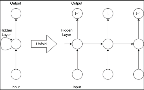
The RNN is a prevalent network structure in deep learning commonly used in sequential learning; it has been used in many studies with convincing results (Tran and Song 2017; Tsai et al. 2018; van der Lugt and Feelders 2019). RNNs are preferred because they make it possible to process an input of any length, account for historical information in the computation process and can have weights shared across time. RNNs allow for previous outputs in their structure to be used as inputs while having a hidden states. The underlying architecture of the RNN is shown in Fig. 1. The architecture of the RNN consists of one input unit, one output unit and one hidden layer, which is the memory of the network (Fig. 1). In the RNN shown in Fig. 1, ‘t – 1’ represents previous values, ‘t’ represents present values and ‘t + 1’ represents future values. The number of unfolded layers depends on the values in the sequence.
|
RNNs build complex non-linear models by iteratively calculating model parameters using algorithms like gradient descent to minimise a loss function, namely, the mean squared error. For a loss function L, a single step of gradient descent will modify the model parameter (say W) as shown in Eqn 1:

where α is the learning rate and i is the iteration number. The input sequence is represented by [x1,x2, …, xm], where m is the length of the sequence. The first RNN block is fed the input x1. The input for the next RNN block will be input x2 and the output of the first RNN block. The input of the mth block will be the output of the (m – 1)th block and xm. The output of the mth block will be compared to y, which represents the next number in the sequence. While training such a network, the input is [x1, x2,…,xm] and the output is y.
Feed-forward neural networks
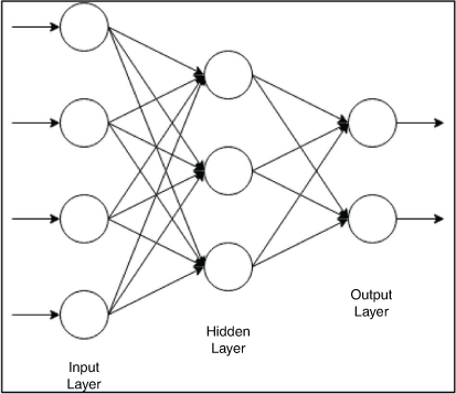
The FFNN is a classification algorithm that consists of several neuron-like processing units organised in layers, with every unit connected to units in the previous layer. The FFNN uses a standard neural network with multiple hidden layers to make a prediction, and can thus be used for time series analysis (Brezak et al. 2012). In the feed-forward system, the signal travels in one direction only from input to output (Ghose et al. 2010). The main advantage of using an FFNN is its ability to make predictions multiple steps ahead; thus, FFNNs are ideally suited to modelling relationships between a set of predictor or input variables and one or more response or output variables. FFNNs have been used in previous studies with considerable success. For example, Farajzadeh et al. (2014) used the autocorrelation regressive integrated moving average (ARIMA) and an FFNN to predict rainfall and water run-off in Urmia Lake basin, Iran. FFNNs are preferred because of their ability to capture complex representations of data in their inputs. Fig. 2 shows a simplified FFNN architecture, with its basic structures.
|
The output in an FFNN layer l in the neural network is given by the following equation:

where a[l] is the number of neurons in a certain layer that determines its dimensions, W[l] and b[l] are the weight matrix and weight vector respectively for layer l, a[l – 1] is the output of the previous layer, f is the activation function (tanh), and tanh is the hyperbolic tangent function.
Water services and economic growth
The relationship between water and economic growth is critical for sustainable planning with regard to water resources, and it is necessary to understand this relationship when evaluating the future of water resources. When water is a bottleneck to the growth of an economy, the provision of either more water, better-controlled water or better-quality water is needed condition for economic growth. As indicated in Table 1, water services directly influence economic activities. Thus, the relationship between water resources and other sectors cannot be segregated if sustainable water practices are to be achieved.
In the agricultural sector, the role of water resources is critical and is looped in to economic growth as well. Agriculture mainly relies on irrigation activities for productivity. This requires huge amounts of water, especially for large-scale activities. The impediment to this activity is nitrate pollution topping highly irrigated areas, making groundwater unusable (Clawson et al. 1971). This often leads to decreased water quality and a shortage of clean water. Decreases in water quality adversely affect water users such as fisheries, as well as decreasing aesthetic values in general. A decrease in agricultural activities, especially for agriculturally driven economies, will negatively affect the economy because there will be less produce for export and a loss of productivity across the population as a result of a decrease in food availability.
Another sector that relies on water services is the energy sector. Water is crucial in hydroelectric schemes for the production of electricity. A constant supply of water improves hydroelectric production, which, in turn, supports the economy. There is a strong link between hydroelectricity and manufacturing: the former provides the energy required to run machines and improve productivity in the latter.
Waste disposal services provided by water resources are of critical importance. The capacity of water to assimilate various types of wastes means that disposal services provided by water resources are vital, especially for industry. Water standards are being set globally for water pollution and, according to Howe (1976), the costs of industrial waste reduction increase sharply as the percentage reduction increases; thus, the capacity of waterbodies to assimilate waste remains a valuable resource.
The importance of municipal water supplies is directly linked to manufacturing, services and the ability to support the population. An affordable and constant supply of municipal water determines the population carrying capacity. With unplanned and strained use of water resources, there could be declines in sanitation and domestic water, resulting in high water costs in a given region. At the microlevel, sewerage and the provision of domestic water can be used to shape urban development trends and growth (e.g. homes being largely built where there is access to water; Chakamera and Alagidede 2018). In the manufacturing and service industries, heavy water users look for ways to ensure their water supply, especially when they require huge amounts of water. The availability of sufficient water from municipal systems can determine the feasibility of a particular industrial location (Howe 1976).
As economic growth takes place, changes in the importance of the services provided by water are inevitable. This underscores the importance of accommodating economic growth through reallocation of existing water supplies while being mindful that existing water laws, the lack of a clear jurisdiction, clear markets and rights to water, especially in the case of transboundary water resources, can stifle sustainable economic growth, particularly when water usage is diminishing the value of an economy. For countries like Egypt, which relies heavily on the Nile River, more specialised agricultural development efforts are more likely to be successful growth initiators than attempts at integrated basin development. This is more important when agricultural expansion is at the heart of regional economic growth in a country. It is also important to note that irrigation is a necessary but not sufficient condition for the initiation of growth of agriculture in arid and semi-arid zones. Therefore, requisite complementary inputs can result in high productivity and growth effects. Even the best predictions of the effects of large water projects on economies and societies contain sufficient uncertainty about ensuing events that the provision of resources for continued monitoring and and evaluation is warranted (Howe 1976).
Materials and methods
Study area
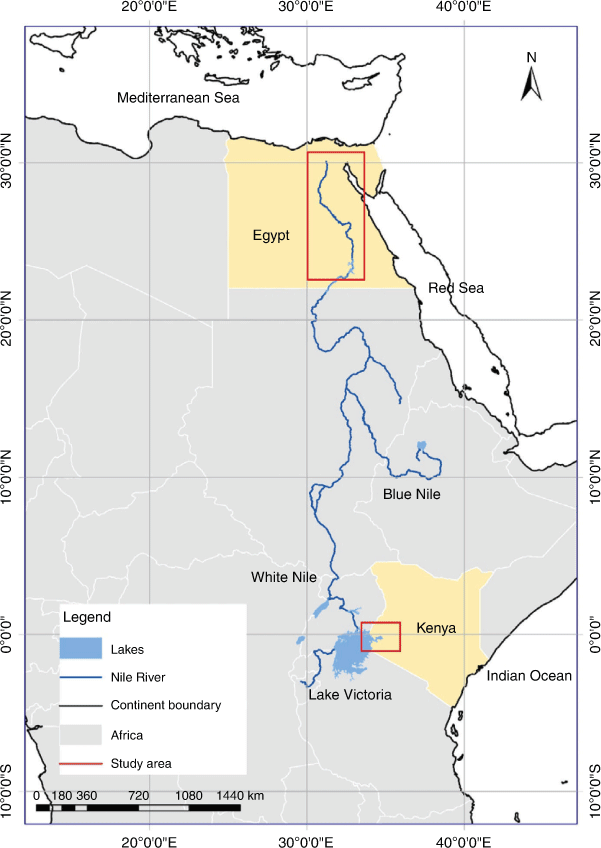
This study was conducted along the Nile River, which has a total length of ~6650 km (4130 miles) between the Lake Victoria and the Mediterranean Sea (Fig. 3). The Nile has a basin drainage area of ~3.35 × 10⁶ km2 and covers 11 countries: Burundi, Tanzania, Rwanda, Kenya, Uganda, Republic of Sudan, Ethiopia, South Sudan, the Democratic Republic of Congo, Eritrea and Egypt (Mumbi and Fengting 2020). Egypt and Sudan are the two major users of the river, and Ethiopia and Kenya harbour the tributaries of the Nile. The flow of the Nile has benefited economic activities in the north-eastern countries through agriculture and tourism. Approximately 80% of the water from the Nile River is used in agricultural activities (Mekonnen and Hoekstra 2014). Complete reliance on water resources throughout the years has caused the Nile River basin to deplete, particularly with regard to essential material resources, with an associated decline in water quality (Rahman 2013; Abdel-Satar et al. 2017). According to Goulden et al. (2009), these changes can be attributed to three factors: a global greenhouse effect resulting from climatic changes, regional factors (e.g. land use) and river basin factors (land management). This argument is consistent with that of Abdel-Satar et al. (2017), who attributed decreases in water quality and depletion along the Nile River to a lack of proper water management interventions, such as hydrodynamic regimes regulated by the Nile barrages; land and water use, including agricultural return; and waste water from industrial, municipal and river ships. In addition to these factors, political tension over ownership rights and user benefits engulf the Nile river basin, particularly in the case of countries that depend on the Nile entirely but are not the source of the Nile (Swain 1997). As in the case of other transboundary resources, conflicts among these countries has been inevitable, with emerging hydropower in the region pushing countries like Egypt and Ethiopia to dominate other countries in this region (Rahman 2013).
|
With previous literature highlighting the importance of undertaking side-by-side analysis such as ours, as opposed to blanket analyses of countries within the Nile (Mumbi and Fengting 2020), two study areas were selected. This study focuses on Kenya and Egypt based on their geopolitical locations in the Nile (Fig. 3). Kenya is located upstream and harbours one of the tributaries of the Nile River, namely the White Nile, which has almost 85% of its water coming from Lake Victoria (FAO Land 1997). Egypt is located downstream and is the drainage point of the Nile as it empties into the Mediterranean Sea. Egypt depends heavily on the Nile, with over 95% of Egyptians living a few kilometres from the Nile River (Nile Basin Initiative 2016). The Nile River has been termed the artery of Egypt, because nearly all the fresh water used for drinking and irrigation in the Egypt comes from the Nile River. The Nile also supplies 65% of industrial water needed in the Egypt and receives 57% of the effluent (Abdel-Satar et al. 2017). With the expansion of industrial, agricultural and recreational activities, in addition to the poorly structured drainage and sewerage systems along the Nile River, both the quality and quantity of water used are of serious concern (Goher et al. 2015).
In addition to the geopolitical aspect in selecting these two countries for evaluation in this study, another strategic aspect is the bilateral cooperation of Egypt and Kenya. Although, unlike Egypt, Kenya does not primarily depend on the Nile River, it is a major player in the Nile basin initiative that promotes cooperation among the countries sharing the Nile. For example, in 2010, Kenya and five other nations, including Ethiopia, signed a River Nile Basin Co-operative Framework agreement. The deal after its ratification by the respective parliaments established a permanent commission to decide on the Nile’s water allocation, albeit without consulting Egypt and Sudan (Kimenyi and Mbaku 2015; Mumbi and Fengting 2020). This, framework was put in place to protect the Nile River and promote peaceful coexistence among the countries that share this resource (Mumbi and Fengting 2020).
Data sources and selection
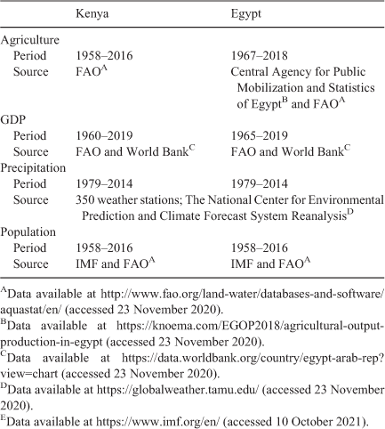
The present study used existing data from different sources. The data were carefully selected, tested, verified and complied before the training process for the neural networks. Owing to the large amount of data used, measures undertaken to ensure trustworthiness during the process included triangulation, peer scrutiny and taking into consideration the background and authority of the sources and publishers (Shenton 2004; Mumbi and Fengting 2020). The data sources and the date range used in this study are provided in Table 2. Evidently, as indicated in Table 2, there were differences periods for data were available and sources between the two countries, which is as expected when dealing with a wide range of data among many countries. Where the required data were missing, extrapolation was done using a basic least squares fit to find intermediate values. The next step was to drop the extra years and equalise the amount of data available between the two countries. In this case, the data cut-off was set at 1979 for both countries. In addition, different data sources were compared to validate the data being used. Data were carefully selected and curated to suit our models, and the data used for training and testing the RNNs and FFNNs are presented in Table 3.
|

|
Data preprocessing and normalisation
Data scaling was conducted before the training process could begin. Data scaling is a recommended preprocessing step when working with neural networks, especially when dealing with different datasets (Brownlee 2019; Nawi et al. 2013). The data used in this study were at different scales and had different distributions both among variables and between the two countries. These differences could increase the difficulty of the modelling process; for example, large input values (e.g. a spread of hundreds or thousands of units) can result in a model that learns large weight values, leading to an unstable model because of the large weights, resulting in higher generalisation error. To overcome this, data scaling is suggested, with a good rule of thumb being small values in the range of 0–1 or standardised with a mean of 0 and a standard deviation of 1 (Brownlee 2019). Data normalisation is a rescaling of the data from the original range so that all values are within the range 0–1.
Because the data used in this study were not normally distributed, data normalisation for the input variables was done, otherwise standardisation would have been an option. The same was done for the output variables plotted and was set to match the activation function (transfer function) on the output layer. The normalisation equation used in this study was:

where the minimum and maximum values pertain to the value x being normalised.
Consequently, the next step was to convert the total water withdrawal data to withdrawal per person. Once data were transformed into the desired input form for the model being trained, data were split into training and test sets (80 and 20% of the dataset respectively).
RNN v. FFNN: performance evaluation and model design
To achieve the objectives of this study, two tasks were conducted. First, both the RNN and FFNN had to be trained before the actual comparison could begin. Second, tests were done to compare the performance of the FFNN and RNN to determine which network to use in the study. There is no rule of thumb for the division of the data to use for training and testing; this varies on case-by-case basis. Many researchers have used different divisions; for example, Boadu (1997) and Kumar et al. (2019) used 80% of their available data for training, Pal (2006) used 69%, Coulibaly and Baldwin (2005) used 90% and Kurup and Dudani (2002) used 63%. In the present study, we used 20% of the available data for testing in both the RNN and FFNN models, as did Boadu (1997) and Kumar et al. (2019).
No precise guidelines govern the proper layout of a neural network. In most cases, analyses that are more intricate require networks that are more complex. However, when the number of free parameters is large, the network will be slower to train and more susceptible to overfitting. Therefore, care should be taken when dealing with complex datasets. To ensure that the models developed in this study would generalise other data, we used regularisation techniques (i.e. L2 regularisation) for the drop-out layers in the RNN and FFNN. The data were also split randomly into training and testing data to ensure that that final model generalises to new data.
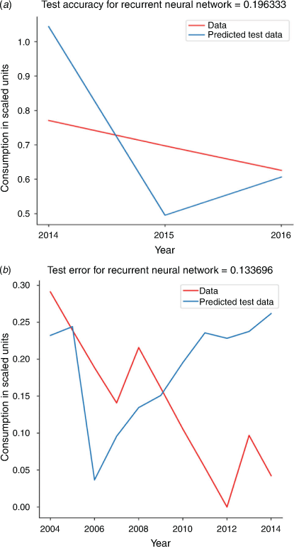
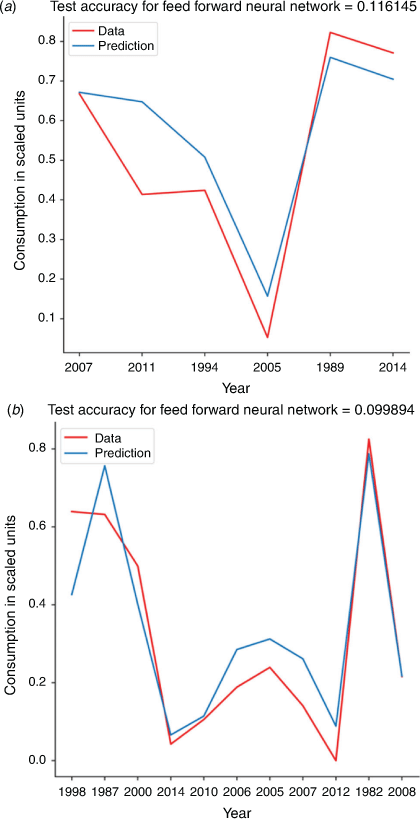
The inputs for predicting the future level of water consumption were prepared using current trends in the first scenario and with GDP doubling in the second scenario. To calculate future inputs, a polynomial fit was performed for each input parameter. Based on the obtained fit, future values were generated. In the second scenario, with GDP doubling, an artificial constraint was used so that the GDP doubled every year while the other three input parameters showed existing trends. The performance of both the RNN and FFNN was evaluated and test accuracy was recorded (Fig. 4 and 5) with the consumption units scaled to between 0 and 1. The final model configuration used was discovered by trial and error, based on skill. This leaves the door open to explore new and possibly better configurations (Kumar et al. 2019). The values of control parameters of the RNN and FFNN were selected initially and thereafter varied in trials until the best fitness measures were produced.
|
|
To investigate the performance of the proposed RNN and FFNN models, the root mean square error (RMSE) was used as a statistical indicator using the following equation and the values reported in Fig. 4 and 5:

RNN model used for the comparison test
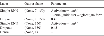
The RNN model was generated using the Keras package (T. Keras, see https://keras.io/api/, accessed 11 October 2021), which is written in Python (see https://www.python.org/doc/, accessed 11 October 2021) (Kingma and Ba 2014). To train the RNN, two dropout layers and one RNN were used. Using Eqn 2, each of the inputs x1,x2,…,xm was four-dimensional, corresponding to the values of GDP, agriculture, population and precipitation that were used for the model. Two layers of RNN were used with dropout layers in between to avoid overfitting (Srivastava et al. 2014). The best results were obtained with a sequence length of 7 and an a[l] with a dimension 30; tanh was used as the activation function and there were 200 training epochs. The mean squared error was used as the loss function to be minimised. The input parameters for the RNN model are given in Table 4.
|
As indicated in Table 4, the output layer was two-dimensional (7 × 150), where 7 corresponds to the sequence length used in the RNN, and so represents the size of the input vector for each training set iteration (this is because each output value depends on a sequence of data points and not just one data point) and 150 represents the number of RNN layers. The probability of a certain hidden unit layer being included in the training is specified in the dropout layer; for example, a dropout of 0.45 indicates that each unit has a 0.45 probability of being included in the training. Most importantly, we used this method for regularisation of the neural network architecture. Consequently, the input for the RNN is a sequence vector of size 4, and a sequence length of 7, where the inputs for each term are specified into four inputs, namely population, agriculture, GDP and precipitation. The RMSE for the RNN was 0.071 × 10³ m3 year–1 for Kenya and 0.897 × 10³ m3 year–1 for Egypt.
Fig. 4 shows the test accuracy for the RNN for modelling water consumption. As shown in Fig. 4, the testing years (x-axis) were randomly drawn from the initial data to make sure that the training data and testing data did not cause any inherent bias to the model. The random predicted values are plotted against the actual values to determine the accuracy of the performance of the model. Fig. 4a shows the test prediction using the RNN for random years 2014–16. As can be seen, the prediction curve deviates considerably from the actual data, indicating that the performance of the RNN was not optimal. The test accuracy of the RNN for Kenya and Egypt was 0.196333 and 0.133696 respectively.
FFNN model used for the comparison test
Similar to the RNN model, the MLP Regressor module in the Sklearn library of Python (see https://www.python.org/doc/) and Keras package (see https://keras.io/api/) was used to build the FFNN model, which was tuned by adjusting the α parameter in the MLP Regressor. To train the FFNN, two hidden layers with one input and one output layer were used. To avoid overfitting, L2 regularisation was used (Krogh and Hertz 1992). The best results were obtained for α = 0.04. Thereafter, the FFNN models were optimised using an Adam optimiser with a learning rate of 0.01 and a tolerance of 1 × 10⁻⁶ (Kingma and Ba 2014). The tolerance rate is a variant of the gradient descent but is more efficient in finding the minima in a multiparameter space. Hyperparameters (see Eqn 2) like the dimension of a[l] the learning rate α, the number of dropout layers, the L2 regularisation parameter and the sequence length m were tuned to obtain the best results. The RMSE for the training data was 0.0689 × 10³ m3 year–1 for Kenya and 0.883 × 10³ m3 year–1 for Egypt.
The test accuracy of the FFNN using data from Kenya and Egypt was 0.116145 and 0.099894 respectively. Fig. 5 shows the test accuracy and errors for the FFNN. Similar to the RNN plots, the testing years were randomly drawn from the initial data to make sure that the training data and testing data did not cause any inherent bias to the model and are plotted along the x-axis. The random predicted values were plotted against the actual values to determine the accuracy of the performance of the model. As shown in Fig. 5, there was not considerable deviation between the predicted values and actual data using the FFNN. Therefore, compared with the RNN, the FFNN performed better and was consequently used in the study.
To model the two proposed scenarios, the inputs for the FFNN model were the independent variables GDP, agriculture, population and precipitation for the first scenario. For the second scenario, with GDP doubling, an artificial constraint was put so that the GDP doubled every year while the other three input parameters showed existing trends. The results of these predictions are elaborated in the Discussion. The loss metric to be minimised was given by the mean squared error using Eqn 4 and as shown below:

where N is the number of data samples, y_model is the predicted value from the model and y_data is the actual value from the data.
Results and discussion
Scenario 1
Water consumption in Kenya
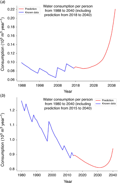
The best results for the FFNN were obtained using 2 hidden layers with 30 hidden units each, with a learning rate of 0.01 and the L2 regularisation parameter set at 0.04. The ranges used were 1–4 hidden layers and 5–50 hidden units in each with a training validation ratio of 80:20. Fig. 6a shows the future prediction for water consumption per person in Kenya per year using an FFNN. The prediction results show a massive increase in water consumption per person steadily over the next 20 years (Fig. 6a). Plausible explanations for this projected increase could be because, according to the Ministry of Water, Sanitation and Irrigation in Kenya, Kenya’s projected per capita water supply is expected to fall to 235 m3 year–1 by 2025 from the current 647 m3 year–1. One of the reasons for this is a projected population increase. As has been observed in the census reports, Kenya’s population is increasing at a very high rate. As expected, an increase in population size leads to more demand for water, not only for direct consumption, but also for use in other sectors, including the agricultural sector, to drive the country’s economy, with Kenya being largely dependent on agricultural exports (Kenya National Bureau of Statistics 2019). Climatic changes are another plausible explanation for this projection. Most parts of Kenya that earlier on used to receive high rainfall are now experiencing less rainfall. This has led to a decline in water levels and, in worst cases, there has been severe drought. Continued mismanagement of the limited water resources poses another challenge in Kenya. With such a projection, Kenya would be expected to come up with strategic policies that are sustainable to protect the country against possible economic collapse, drought and increased water shortages in the future.
|
Water consumption in Egypt
For Egypt, the best results for the FFNN were obtained using 3 hidden layers with 50 hidden units each. A learning rate of 0.01 and an L2 regularisation parameter of 0.1 were used. In Egypt, based on the trend in the previous year, the results show a small decrease in the predicted value at the start up until 2032; thereafter, there is a huge increase in expected water consumption (Fig. 6b). This observed increase can be explained by the geographical location of Egypt. Egypt receives <80 mm of rainfall per year and only 6% of its land is arable, with the rest mostly desert. With the country relying heavily on agriculture, and given the low supply of water from its sources, water demand in the agriculture sector is bound to increase if the sector is to stay afloat. This is similar to previous studies, which have estimated that Egypt’s demand for water will exceed supply within the next few years (Wehling 2020a). Another plausible explanation is the steep population growth in the country, which is associated with a correspondingly steep rise in demand for water for agricultural, domestic and industrial use. Egypt is one of the countries whose economy would be severely affected if countries upstream on the Nile River interfered with water flow because of its reliance on hydropower and its need for water (Wehling 2020a).
As stated earlier, the primary source of water in Egypt is the Nile River with almost the entire population completely dependent on the Nile water (Gad 2017: Wehling 2020a). In addition to the Nile River, the water supply for agriculture in Egypt is supplemented to a very small extent by rainfall and groundwater. The agriculture sector is crucial for Egypt because it adds up to 14.5% to the country’s GDP, provides a livelihood for 29.6% of the population and accounts for 11% of exports (Gad 2017), but it uses 85% of Egypt’s water. Although the government in Egypt has reduced the cultivation of high water-consuming crops like rice because of increasing water demand, demand for both water and food has risen due to population growth, which itself has triggered agricultural development and increased industrial activity in the country (Gad 2017). Over the years, Egypt has had major control over water use in the Nile because of a colonial-era treaty that guaranteed Egypt a 90% share of water in the Nile River and prevented the other users of the Nile River from extracting water without Egypt’s permission (Wehling 2020a). However, with countries like Ethiopia building dams upstream, Egypt has valid concerns is that this could decrease the amount of water it receives. A reduction in water supply from the Nile River will hinder Egypt’s efforts to alleviate water shortages in the dry months in the country (Wehling 2020a).
Scenario 2
Doubling GDP for Kenya
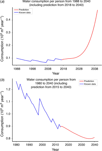
Scenario 2 considered an expected increase in the GDP. This scenario assumes no change in the other variables affecting water consumption. Given the current trends, especially in Kenya, where the economy has been increasing, it is only rational to assume that the trend would maintain an upward projection over the coming years. As shown in Fig. 7a, the projected water demand in Kenya increases to 0.5 units with time to 2040.
|
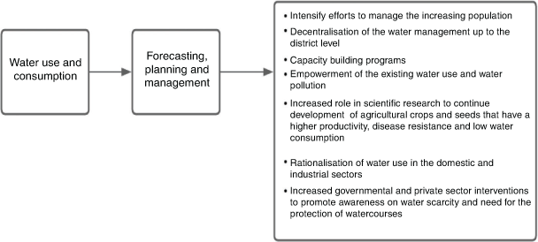
These results indicate that unless urgent steps are taken to control population growth, rehabilitate irrigation and water supply networks and rationalise water use, it will be difficult to provide enough water for economic expansion and growth in the future. Therefore, Kenya, needs to consider alternative measures, such as water recycling or water-saving technologies, especially in the industrial sector, to curb any possible future shortages that would be brought about by the ambitious economic growth.
Doubling GDP for Egypt
In the case of Egypt, as shown in Fig. 7b, doubling the GDP results in a significant decrease in the curve following the previous year’s trajectory, which is then followed by an increase to 0.8 m3 of water consumption per person in 2040. A plausible explanation for the observed pattern is that, although economic growth accounts for most water use in Egypt, agriculture has been proven to be the main factor controlling water demand in Egypt, followed by tourism as observed by Ahmed et al. (2014) in their study of water use at Luxor, Egypt. Thus, the reverse pattern in predicted water consumption per person would have been observed if water use in the agricultural sector had been doubled while the other factors were kept constant. Based on the observed results, there should be enhanced sharing and cooperation of various water users in Egypt for integrated management of future water demand (Ahmed et al. 2014). Therefore, Egypt should strive to ensure water balance among different sectors. Furthermore, with expectations of climate conditions becoming drier and upstream countries continuing to increase their use of Nile waters, Egypt cannot afford to neglect the importance of water conservation anymore and must act immediately to augment its natural water reserves (Wehling 2020b).
Implications of the study, global outlook and future studies
Many countries may face water resources-based vulnerability under expected global changes (Kulshreshtha 1998). With a continued decrease in the amount of renewable global water resources, there is a need for forecasting to aid proper development and planning. Moreover, climate change and changes in water withdrawal could aggravate water resource stress worldwide. Understanding possible changes and likely scenarios using tools such as forecasting is critical for future planning and resources management. Forecasting both long- and short-term outcomes necessitates explicit judgements about economic forces that matter and those that do not (Brandt and Rawski 2008; Perkins and Rawski 2008). Although both long-term (>20 years) and short-term (1–2 years) forecasting are important, long-term forecasting is preferred because it is largely independent of sudden shocks or short-term behaviours and is driven primarily by the growth rate, development and expenditure (Perkins and Rawski 2008), which is why we used long-term forecasting in the present study.
Globally, the effects of global warming on the hydrological cycle have been studied and documented (Houghton 1996; Arnell 2004; Oki and Kanae 2006). With a projected increase in global water demand, it is imperative to have informed policies and governing structures in place, mainly because the global water crisis is more of a governance issue rather than the result of the actual availability of the resource (Steduto et al. 2012). This will promote effective rules for the sustainable utilisation and protection of international water, especially transboundary resources that are shared by many countries. With more than half the world’s 263 transboundary water basins still not covered by a framework between the riparian states to regulate cooperation in water management, the countries that harbour these resources are set for a catastrophic future given the forecast decline in the potential of these resources (Connor 2015). Similar to other riparian states in the world that have already signed water agreements, efforts should be made to have basin-wide treaties in place for important transboundary watercourses such as the Nile, Jordan, Tigris and Euphrates rivers to promote a general framework for basin users (Wehling 2020b).
As shown in Fig. 8, given the forecast trajectory of water demand through consumption in Kenya and Egypt, caution should be observed with regard to water use in these countries and the measures suggested in Fig. 8 should be implemented. Based on the results of this study, we suggest measures that can be adapted to help promote sustainable water use practices in the Nile basin region, as well as for other transboundary water resources around the world. In addition, based on this study, there should be an emphasis on understanding water usage in all sectors so that appropriate efforts and measures can be allocated to ensure that water demand in the different sectors is met and that water resources are equally distributed. More so, dissemination of information on issues around water scarcity should be a priority to ensure the uptake of water behaviours such as water recycling and the proper use of the limited available resources.
|
This study identifies existing gaps and recommends a few measures for future studies. This study focused on a transboundary resource in one upstream (Kenya) and one downstream (Egypt) country, but the impacts of both political and social water use in countries between Kenya and Egypt on the projections cannot be ignored. Such issues in other countries were not investigated in this study, but could be followed-up in future studies. Using a similar approach in the other countries in the region that were not part of the present study will aid our understanding of the implications of the current trends in water use and help with the development of management models and strategies being adopted by the Nile basin initiative, making them more efficient and accurate.
Another important contribution of this study is the development of a model that uses a combination of different input data to model a singular output (i.e. water demand) that can be interpreted and help with better planning. Future studies should use this methodology in other geographical areas, sectors, resources or transboundary waterbodies to forecast and promote sustainable resource utilisation.
Research such as ours provides a snapshot of the future given continued trends. With such information, other transboundary countries can replicate our model and use the information obtained to develop compact management models and to strengthen existing management models. We also recommend creating many hypothetical scenarios (e.g. accounting for changes in other variables, not only GDP) and analysing their effects on water demand by forming a grid of values for different variables and observing changes in them.
Study limitations
This study analysed water resources and their use on a country-by-country basis. There are a few limitations that should not be overlooked. This study did not include water usage and interrelationships for human activities such as the recreational sector, which is popular in Egypt, where the Nile River supports cruising activities. Another limitation of the study lies in the selection of variables, with only the effect of doubling the GDP evaluated while the other variables were kept constant. It should be noted that changes in the population, for example, may have a considerable effect on the GDP and interact with other sectors that rely heavily on water usage. These are some prominent gaps in the study that should be considered in future work. Finally, information at the country level regarding water use is poor, with outdated figures and data lacking in some sectors. Attempts should be made to develop appropriate datasets for a comprehensive assessment of water resources, especially in developing nations.
Conclusion
In this study, FFNN was used to make a long-term forecast of water demand along the Nile River in two countries (Egypt and Kenya) up to the year 2040. This was done through understanding the complex relationship between different sectors (i.e. intensive urbanisation, booming population, climate change and water use in the agricultural sector) for the proper planning and management of transboundary water resources. From the results, it is evident that the FFNN performed better than the RNN during the testing process and can be used as a reliable machine learning technique for various studies and other phenomena, such as hydrological or rainfall forecasting. A scenario in which the GDP was doubled was also modelled in both countries, and its effects on per-person water intake were observed while water consumption in the other sectors was held constant. The results of the first scenario indicate that, in Kenya, given the current trends, water consumption is forecast to increase steadily to 2040, whereas the reverse was observed in Egypt, with a decrease in water consumption followed by a slight increase. When the GDP in both countries was doubled in the Scenario 2, the forecast in Kenya is for an immediate increase in water consumption, whereas in Egypt the water consumption trend continues in its current state, decreases and then increases again just before 2040. From these results, it is clear that conducting time series analysis is of great significance, because it provides a snapshot of future expectations. This can offer timely strategies for the management of water resources and provide long-lasting solutions.
Author contributions
All authors were fully involved in drafting the manuscript, writing it and approving the final version for publication.
Conflicts of interest
The authors declare that they have no conflicts of interest.
Declaration of funding
This research received no external funding.
Acknowledgements
The authors are very grateful for the valuable comments and suggestions made by colleagues at Tongji University. The Authors are particularly grateful to Dr Jie Yu from the College of Surveying and Geo-informatics at Tongji University for the assistance provided in editing the map used in this study.
References
Abdel-Satar, A. M., Ali, M. H., and Goher, M. E. (2017). Indices of water quality and metal pollution of Nile River, Egypt. Egyptian Journal of Aquatic Research 43, 21–29.| Indices of water quality and metal pollution of Nile River, Egypt.Crossref | GoogleScholarGoogle Scholar |
Adamowski, J. F. (2008). Peak daily water demand forecast modeling using artificial neural networks. Journal of Water Resources Planning and Management 134, 119–128.
| Peak daily water demand forecast modeling using artificial neural networks.Crossref | GoogleScholarGoogle Scholar |
Adamowski, J., and Karapataki, C. (2010). Comparison of multivariate regression and artificial neural networks for peak urban water-demand forecasting: evaluation of different ANN learning algorithms. Journal of Hydrologic Engineering 15, 729–743.
| Comparison of multivariate regression and artificial neural networks for peak urban water-demand forecasting: evaluation of different ANN learning algorithms.Crossref | GoogleScholarGoogle Scholar |
Ahmed, A. A., Fogg, G. E., and Gameh, M. A. (2014). Water use at Luxor, Egypt: consumption analysis and future demand forecasting. Environmental Earth Sciences 72, 1041–1053.
| Water use at Luxor, Egypt: consumption analysis and future demand forecasting.Crossref | GoogleScholarGoogle Scholar |
Allan, J. A. (2009) Nile basin asymmetries: a closed fresh water resource, soil water potential, the political economy and Nile transboundary hydropolitics. In ‘The Nile’. pp. 749–770. (Springer)
Arbués, F., Garcıa-Valiñas, M. Á., and Martınez-Espiñeira, R. J. (2003). Estimation of residential water demand: a state-of-the-art review. Journal of Socio-Economics 32, 81–102.
| Estimation of residential water demand: a state-of-the-art review.Crossref | GoogleScholarGoogle Scholar |
Arnell, N. W. (2004). Climate change and global water resources: Sres emissions and socio-economic scenarios. Global Environmental Change 14, 31–52.
| Climate change and global water resources: Sres emissions and socio-economic scenarios.Crossref | GoogleScholarGoogle Scholar |
Asaminev, A. C., Denghua, Y., Xinshan, S., Hao, W., Dorjsuren, B., Abel, G., Baisha, W., and Tianlin, Q. (2020). Assessing the impact of climate change on hydro-ecological processes of the Abbay River Basin in Ethiopia. Молодой ученый 50, 394–402.
Bastiaanssen, W. G., Karimi, P., Rebelo, L.-M., Duan, Z., Senay, G., Muthuwatte, L., and Smakhtin, V. (2014). Earth observation based assessment of the water production and water consumption of Nile Basin agro-ecosystems. Remote Sensing 6, 10306–10334.
| Earth observation based assessment of the water production and water consumption of Nile Basin agro-ecosystems.Crossref | GoogleScholarGoogle Scholar |
Baumann, D. D., Boland, J., and Hanemann, W. M. (1998). ‘Urban Water Demand Management and Planning’ (McGraw-Hill: New York, NY, USA.)
Bierkens, M. F., Knotters, M., and Hoogland, T. (2001). Space‐time modeling of water table depth using a regionalized time series model and the Kalman Filter. Water Resources Research 37, 1277–1290.
| Space‐time modeling of water table depth using a regionalized time series model and the Kalman Filter.Crossref | GoogleScholarGoogle Scholar |
Boadu, F. K. (1997). Rock properties and seismic attenuation: neural network analysis. Pure and Applied Geophysics 149, 507–524.
| Rock properties and seismic attenuation: neural network analysis.Crossref | GoogleScholarGoogle Scholar |
Boretti, A., and Rosa, L. (2019). Reassessing the projections of the world water development report. NPJ Clean Water 2, 15.
| Reassessing the projections of the world water development report.Crossref | GoogleScholarGoogle Scholar |
Brandt, L., and Rawski, T. G. (2008). ‘China’s Great Economic Transformation.’ (Cambridge University Press.)
Brezak, D., Bacek, T., Majetic, D., Kasac, J., and Novakovic, B. (2012). A comparison of feed-forward and recurrent neural networks in time series forecasting. In ‘2012 IEEE Conference on Computational Intelligence for Financial Engineering & Economics (CIFEr)’, 2012, pp. 1–6. (IEEE)
Brownlee, J. (2019). How to scale data for long short-term memory networks in Python. (Machine Learning Mastery.) Available at https://machinelearningmastery.com/how-to-scale-data-for-long-short-term-memory-networks-in-python/ [Verified 11 October 2021].
Chakamera, C., and Alagidede, P. (2018). The nexus between infrastructure (quantity and quality) and economic growth in Sub-Saharan Africa. International Review of Applied Economics 32, 641–672.
| The nexus between infrastructure (quantity and quality) and economic growth in Sub-Saharan Africa.Crossref | GoogleScholarGoogle Scholar |
Chen, S., and Hu, X. (2018). Individual identification using the functional brain fingerprint detected by the recurrent neural network. Brain Connectivity 8, 197–204.
| Individual identification using the functional brain fingerprint detected by the recurrent neural network.Crossref | GoogleScholarGoogle Scholar | 29634323PubMed |
Clawson, M., Landsberg, H. H., and Alexander, L. T. (1971). The agricultural potential of the middle east. In ‘The agricultural potential of the Middle East’. (Elsevier Science: New York, NY, USA.)
Connor, R. (2015). ‘The United Nations World Water Development Report 2015: Water for a Sustainable World.’ (UNESCO Publishing)
Coulibaly, P., and Baldwin, C. K. (2005). Nonstationary hydrological time series forecasting using nonlinear dynamic methods. Journal of Hydrology 307, 164–174.
| Nonstationary hydrological time series forecasting using nonlinear dynamic methods.Crossref | GoogleScholarGoogle Scholar |
FAO Land (1997). Irrigation potential in Africa; a basin approach. Land and Water Bulletin number 4. (Food and Agriculture Organization of the United Nations: Rome, Italy.) Available at http://www.fao.org/docrep/ W4347E/w4347e00.htm#Contents
Farajzadeh, J., Fard, A. F., and Lotfi, S. (2014). Modeling of monthly rainfall and runoff of Urmia Lake Basin using ‘feed-forward neural network’ and ‘time series analysis’ model. Water Resources and Industry 7–8, 38–48.
| Modeling of monthly rainfall and runoff of Urmia Lake Basin using ‘feed-forward neural network’ and ‘time series analysis’ model.Crossref | GoogleScholarGoogle Scholar |
Gad, W. A. (2017). Water scarcity in Egypt: causes and consequences. The IIOAB Journal 8, 40–47.
Ghose, D. K., Panda, S. S., and Swain, P. C. (2010). Prediction of water table depth in western region, Orissa using BPNN and RBFN neural networks. Journal of Hydrology 394, 296–304.
| Prediction of water table depth in western region, Orissa using BPNN and RBFN neural networks.Crossref | GoogleScholarGoogle Scholar |
Goher, M. E., Abdo, M. H., Mangood, A. H., and Hussein, M. M. (2015). Water quality and potential health risk assessment for consumption of Oreochromis niloticus from el-Bahr el-Pharaony Drain, Egypt. Fresenius Environmental Bulletin 24, 3590–3602.
Goulden, M., Conway, D., and Persechino, A. (2009). Adaptation to climate change in international river basins in Africa: a review. Hydrological Sciences Journal 54, 805–828.
| Adaptation to climate change in international river basins in Africa: a review.Crossref | GoogleScholarGoogle Scholar |
Hamouda, M. A., El-Din, M. M. N., and Moursy, F. I. (2009). Vulnerability assessment of water resources systems in the eastern Nile Basin. Water Resources Management 23, 2697–2725.
| Vulnerability assessment of water resources systems in the eastern Nile Basin.Crossref | GoogleScholarGoogle Scholar |
Herrera, M., Torgo, L., Izquierdo, J., and Pérez-García, R. (2010). Predictive models for forecasting hourly urban water demand. Journal of Hydrology 387, 141–150.
| Predictive models for forecasting hourly urban water demand.Crossref | GoogleScholarGoogle Scholar |
Houghton, E. (1996). ‘Climate Change 1995: the Science of Climate Change: Contribution of Working Group I to the Second Assessment Report of the Intergovernmental Panel On Climate Change’ (Cambridge University Press: New York, NY, USA.)
Howe, C. W. (1976). The effects of water resource development on economic growth the conditions for success. Natural Resources Journal 16, 939–955.
Kenya National Bureau of Statistics (2019). 2019 Kenya population and housing census. Available at https://housingfinanceafrica.org/documents/2019-kenya-population-and-housing-census-reports/
Kheireldin, A. T. (2016). Using the water-energy-food nexus to enhance Egypt’s cooperation with Nile basin countries. Thesis, American University in Cairo, Sustainable Development. Available at http://dar.aucegypt.edu/handle/10526/4745
Kimenyi, M. S., and Mbaku, J. M. (2015). The limits of the new ‘Nile Agreement’. In ‘Africa in Focus’, 28 April 2015. (The Brookings Institution.) Available at https://www.brookings.edu/blog/africa-in-focus/2015/04/28/the-limits-of-the-new-nile-agreement/
Kingma D. P.Ba J. (2014 ). Adam: A method for stochastic optimization. arXiv preprint 1412.6980.
Kliot, N., Shmueli, D., and Shamir, U. (2001). Institutions for management of transboundary water resources: their nature, characteristics and shortcomings. Water Policy 3, 229–255.
| Institutions for management of transboundary water resources: their nature, characteristics and shortcomings.Crossref | GoogleScholarGoogle Scholar |
Krogh, A., and Hertz, J. A. (1992). A simple weight decay can improve generalization. In ‘Advances in Neural Information Processing Systems’. Vol. 4, pp. 950–957. (Morgan Kaufmann Publishers: San Mateo, CA, USA.)
Kulshreshtha, S. N. (1998). A global outlook for water resources to the year 2025. Water Resources Management 12, 167–184.
| A global outlook for water resources to the year 2025.Crossref | GoogleScholarGoogle Scholar |
Kumar, D., Singh, A., Samui, P., and Jha, R. K. (2019). Forecasting monthly precipitation using sequential modelling. Hydrological Sciences Journal 64, 690–700.
| Forecasting monthly precipitation using sequential modelling.Crossref | GoogleScholarGoogle Scholar |
Kurup, P. U., and Dudani, N. K. (2002). Neural networks for profiling stress history of clays from PCPT data. Journal of Geotechnical and Geoenvironmental Engineering 128, 569–579.
| Neural networks for profiling stress history of clays from PCPT data.Crossref | GoogleScholarGoogle Scholar |
Lee, D., and Derrible, S. (2020). Predicting residential water demand with machine-based statistical learning. Journal of Water Resources Planning and Management 146, 04019067.
| Predicting residential water demand with machine-based statistical learning.Crossref | GoogleScholarGoogle Scholar |
McCracken, M., and Wolf, A. T. (2019). Updating the register of international river basins of the world. International Journal of Water Resources Development 35, 732–782.
| Updating the register of international river basins of the world.Crossref | GoogleScholarGoogle Scholar |
Mekonnen, M. M., and Hoekstra, A. Y. (2014). Water conservation through trade: the case of Kenya. Water International 39, 451–468.
| Water conservation through trade: the case of Kenya.Crossref | GoogleScholarGoogle Scholar |
Mumbi, A. W., and Fengting, L. (2020). Exploring changes in water use patterns, demand and stress along the Nile River Basin through the lens of Kenya and Egypt. Marine and Freshwater Research 71, 1478–1487.
| Exploring changes in water use patterns, demand and stress along the Nile River Basin through the lens of Kenya and Egypt.Crossref | GoogleScholarGoogle Scholar |
Nawi, N. M., Atomi, W. H., and Rehman, M. Z. (2013). The effect of data pre-processing on optimized training of artificial neural networks. Procedia Technology 11, 32–39.
| The effect of data pre-processing on optimized training of artificial neural networks.Crossref | GoogleScholarGoogle Scholar |
Nelson, P. J., Nyarangi, J., Maritim, Z. K., Teferi, T., Awer, M., Awale, B., Hamisi, S., Nkako, F. O., Gichangi, K., Kasanga, W., et al. (2012). The trans-boundary Mara River Basin strategic environmental assessment (MRB SEA). Report prepared for LVBC, WWF, USAID and the Governments of Tanzania and Kenya. (Earth Interactions.) Available at http://repository.eac.int/bitstream/handle/11671/708/The%20Trans-Boundary%20Mara%20River%20Basin%20Strategic%20Environmental%20Assessment.pdf?sequence=1&isAllowed=y [Verified 18 October 2021].
Nile Basin Initiative (2016). Building on shared benefits: transforming lives in the Nile Basin. (Nile Basin Initiative Secretariat (Nile-SEC): Entebbe, Uganda.) Available at https://www.nilebasin.org/index.php/our-story/95-keeping-the-nile-flowing-and-boosting-livelihoods-2
Oki, T., and Kanae, S. (2006). Global hydrological cycles and world water resources. The Science of the Total Environment 313, 1068–1072.
Pal, M. (2006). Support vector machines‐based modelling of seismic liquefaction potential. International Journal for Numerical and Analytical Methods in Geomechanics 30, 983–996.
| Support vector machines‐based modelling of seismic liquefaction potential.Crossref | GoogleScholarGoogle Scholar |
Perkins, D. H., and Rawski, T. G. (2008). Forecasting China’s economic growth over the next two decades. In ‘China’s Great Economic Transformation’ (Eds L. Brandt and T. G. Rawski.) Ch. 20, pp. 829–886. (Cambridge University Press.)
Pfister, S., Bayer, P., Koehler, A., and Hellweg, S. (2011). Projected water consumption in future global agriculture: Scenarios and related impacts. The Science of the Total Environment 409, 4206–4216.
| Projected water consumption in future global agriculture: Scenarios and related impacts.Crossref | GoogleScholarGoogle Scholar | 21840571PubMed |
Pranav, E., Kamal, S., Chandran, C. S., and Supriya, M. (2020). Facial emotion recognition using deep convolutional neural network. In ‘2020 6th International Conference on Advanced Computing and Communication Systems (ICACCS)’, 6–7 March 2020, Coimbatore, India. pp. 317–320. (IEEE.)
Rahman, M. A. (2013). Water security: Ethiopia–Egypt transboundary challenges over the Nile River Basin. Journal of Asian and African Studies 48, 35–46.
| Water security: Ethiopia–Egypt transboundary challenges over the Nile River Basin.Crossref | GoogleScholarGoogle Scholar |
Savenije, H. H., and Van der Zaag, P. (2000). Conceptual framework for the management of shared river basins; with special reference to the SADC and EU. Water Policy 2, 9–45.
| Conceptual framework for the management of shared river basins; with special reference to the SADC and EU.Crossref | GoogleScholarGoogle Scholar |
Shenton, A. K. (2004). Strategies for ensuring trustworthiness in qualitative research projects. Education for Information 22, 63–75.
| Strategies for ensuring trustworthiness in qualitative research projects.Crossref | GoogleScholarGoogle Scholar |
Srivastava, N., Hinton, G., Krizhevsky, A., Sutskever, I., and Salakhutdinov, R. (2014). Dropout: a simple way to prevent neural networks from overfitting. Journal of Machine Learning Research 15, 1929–1958.
Steduto, P., Faurès, J.-M., Hoogeveen, J., Winpenny, J., and Burke, J. (2012). Coping with water scarcity: An action framework for agriculture and food security. Journal of FAO Water Reports 16, 78.
Swain, A. (1997). Ethiopia, the Sudan, and Egypt: the Nile River dispute. The Journal of Modern African Studies 35, 675–694.
| Ethiopia, the Sudan, and Egypt: the Nile River dispute.Crossref | GoogleScholarGoogle Scholar |
Tilman, D., Fargione, J., Wolff, B., D’antonio, C., Dobson, A., Howarth, R., Schindler, D., Schlesinger, W. H., Simberloff, D., and Swackhamer, D. (2001). Forecasting agriculturally driven global environmental change. The Science of the Total Environment 292, 281–284.
Tran, Q.-K., and Song, S.-K. (2017). Water level forecasting based on deep learning: a use case of Trinity River, Texas, the United States. Journal of KIISE 44, 607–612.
| Water level forecasting based on deep learning: a use case of Trinity River, Texas, the United States.Crossref | GoogleScholarGoogle Scholar |
Tsai, Y.-T., Zeng, Y.-R., and Chang, Y.-S. (2018). Air pollution forecasting using RNN with LSTM. In ‘2018 IEEE 16th International Conference on Dependable, Autonomic and Secure Computing, 16th International Conference on Pervasive Intelligence and Computing, 4th International Conference on Big Data Intelligence and Computing and Cyber Science and Technology Congress (DASC/PiCom/DataCom/CyberSciTech)’, 12–15 August 2018, Athens, Greece. pp. 1074–1079. (IEEE.) Available at http://cyber-science.org/2018/dasc/
van der Lugt, B. J., and Feelders, A. J. (2019). Conditional forecasting of water level time series with RNNS. In ‘International Workshop on Advanced Analysis and Learning on Temporal Data’. pp. 55–71. (Springer.)
Wada, Y., Flörke, M., Hanasaki, N., Eisner, S., Fischer, G., Tramberend, S., Satoh, Y., Van Vliet, M., Yillia, P., and Ringler, C. J. G. M. D. (2016). Modeling global water use for the 21st century: the water futures and solutions (WFAS) initiative and its approaches. Geoscientific Model Development 9, 175–222.
| Modeling global water use for the 21st century: the water futures and solutions (WFAS) initiative and its approaches.Crossref | GoogleScholarGoogle Scholar |
Wehling, P. (2020a). ‘Nile Water Rights.’ (Springer.)
Wehling, P. (2020b). The Nile and its catchment area. In ‘Nile Water Rights’. pp. 95–103. (Springer.)
Yue, Z., Alun, G., and Bolin, P. (2017). Relationship between industrial water consumption and economic growth in China based on environmental Kuznets curve. Energy Procedia 105, 3557–3564.
| Relationship between industrial water consumption and economic growth in China based on environmental Kuznets curve.Crossref | GoogleScholarGoogle Scholar |
Zhao, X., Fan, X., and Liang, J. (2017). Kuznets type relationship between water use and economic growth in China. Journal of Cleaner Production 168, 1091–1100.
| Kuznets type relationship between water use and economic growth in China.Crossref | GoogleScholarGoogle Scholar |
Zhou, S. L., McMahon, T. A., Walton, A., and Lewis, J. (2000). Forecasting daily urban water demand: a case study of Melbourne. Journal of Hydrology 236, 153–164.
| Forecasting daily urban water demand: a case study of Melbourne.Crossref | GoogleScholarGoogle Scholar |
Zubaidi, S. L., Ortega-Martorell, S., Al-Bugharbee, H., Olier, I., Hashim, K. S., Gharghan, S. K., Kot, P., and Al-Khaddar, R. (2020). Urban water demand prediction for a city that suffers from climate change and population growth: Gauteng Province case study. Water 12, 1885.
| Urban water demand prediction for a city that suffers from climate change and population growth: Gauteng Province case study.Crossref | GoogleScholarGoogle Scholar |


