
Seasonal climate summary for the southern hemisphere (spring 2018): positive Indian Ocean Dipole and Australia’s driest September on record
Blair Trewin
A Bureau of Meteorology, GPO Box 1289, Melbourne, Vic. 3001, Australia. Email: blair.trewin@bom.gov.au
Journal of Southern Hemisphere Earth Systems Science 70(1) 373-392 https://doi.org/10.1071/ES20007
Submitted: 24 August 2020 Accepted: 8 October 2020 Published: 19 November 2020
Journal Compilation © BoM 2020 Open Access CC BY-NC-ND
Abstract
This is a summary of the southern hemisphere atmospheric circulation patterns and meteorological indices for spring 2018; an account of seasonal rainfall and temperature for the Australian region and broader southern hemisphere is also provided. A positive phase of the Indian Ocean Dipole developed during the season, and the central and eastern equatorial Pacific were warmer than average without reaching El Niño thresholds. It was Australia’s driest September on record, before rainfall of closer to average in October and November. It was warmer than average, especially in northern Australia, with coastal Queensland affected by extreme heat and wildfires in November. It was one of the three warmest springs on record for the southern hemisphere as a whole, and was notably dry in southern and eastern Africa.
Keywords: Australia, driest September, equatorial Pacific, extreme heat, Indian Ocean Dipole, sea-surface temperature.
1 Introduction
This summary reviews the southern hemisphere and equatorial climate patterns for spring 2018, with particular attention given to the Australasian and equatorial regions of the Pacific and Indian ocean basins. The main sources of information for this report are analyses prepared by the Australian Bureau of Meteorology, with data also obtained from other agencies outside Australia.
2 Pacific and Indian ocean basin climate indices
2.1 Southern Oscillation Index (SOI)
The Troup SOI1 for the period from January 2014 to November 2018 is shown in Fig. 1; also shown is a five-month weighted, moving average of the monthly SOI. The seasonal mean value of the SOI for spring 2018 was −2.4, rising from −10.0 in September to near or above zero in October and November.

|
Sustained negative values of SOI below –7 are often indicative of El Niño episodes, while persistently positive values of SOI above +7 are typical of a La Niña episode. Most monthly SOI values in 2018 were between +7 and −7, consistent with a neutral state of the El Niño Southern Oscillation (ENSO) following a weak La Niña event in late 2017 and early 2018, which ended in March (Chapman and Rosemond 2020).
2.2 Composite monthly ENSO index (5VAR) and other ENSO indices
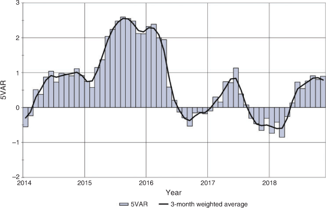
The ENSO 5VAR Index2 is a composite monthly ENSO index, calculated as the standardised amplitude of the first principal component of the monthly Darwin and Tahiti mean sea level pressure (MSLP) and monthly indices NINO3, NINO3.4 and NINO4 sea-surface temperatures3 (SSTs). Values of the 5VAR that are in excess of one standard deviation are typically associated with El Niño for positive values, while negative 5VAR values of a similar magnitude are indicative of La Niña.
Positive values of the 5VAR index persisted throughout spring 2018 (Fig. 2), with values in the range from +0.8 to +0.9 in all three months, consistent with conditions near the threshold of an El Niño. The Bureau of Meteorology did not declare an El Niño during the period, but some other agencies, such as the U.S. National Oceanic and Atmospheric Administration (NOAA), did classify it as the start of a weak El Niño event.
|
The Multivariate ENSO Index (MEI)4 version 2, produced by the NOAA Physical Sciences Laboratory, is derived from five atmospheric and oceanic parameters calculated as a two-month mean (Wolter and Timlin 2011). As with 5VAR, large negative anomalies in the MEI are usually associated with La Niña and large positive anomalies with El Niño. The September–October (+0.4) and October–November (+0.3) values were consistent with a neutral state of ENSO.
The NINO3.4 index, which measures SSTs in the central Pacific Ocean between 5°N–5°S and 120–170°W, is used by the Australian Bureau of Meteorology to monitor ENSO; NINO3.4 is closely related to the Australian climate (Wang and Hendon 2007). NINO3.4 warmed from 0.4°C to 0.8°C, near the threshold for declaration of an El Niño, in October and November.
2.3 Indian Ocean Dipole (IOD)
The IOD5 is the difference in ocean temperatures from the western node of the tropical Indian Ocean (centred on the Equator) off the coast of Somalia and the eastern node off the coast of Sumatra. The IOD is said to be in a positive phase when values of the Dipole Mode Index (DMI) are greater than 0.4°C, neutral when the DMI is sustained between –0.4°C and 0.4°C and negative when DMI values are less than –0.4°C.
When under the influence of a strongly negative IOD phase, warm maritime air is driven eastwards across the continent, leading to negative IOD typically being associated with an increased chance of a wetter than average spring and/or winter for much of the continent. Conversely, positive IOD events are typically associated with dry conditions (Ummenhofer et al. 2009). Negative IOD events often occur in conjunction with La Niña in the Pacific Ocean,6 and positive IOD with El Niño; that the two phenomena are related is acknowledged, but the relationship between ENSO and the IOD is complicated (Meyers et al. 2007; Wang and Wang 2014) and continues to be an active area of research. An IOD event of positive or negative phase may have a significant influence on rainfall regimes for Australia, as well as other parts of the Indian Ocean region, particularly Indonesia and East Africa.
A positive phase of the IOD developed during spring 2018. Rapid development occurred in September, with weekly DMI values peaking near 0.8°C (Fig. 3). The DMI was then consistently near the DMI threshold of 0.4°C in October and November before falling below threshold levels in early December. The positive phase of the IOD contributed to dry conditions in many parts of the Australian continent in September, as well as below-average rainfall in parts of the Maritime Continent region, particularly parts of Java.

|
3 Outgoing longwave radiation (OLR)
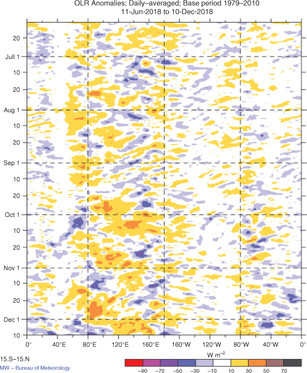
The OLR in the equatorial Pacific Ocean can be used as an indicator of enhanced or suppressed tropical convection. Increased positive OLR anomalies typify a regime of reduced convective activity, a reduction in cloudiness and, usually, rainfall. Conversely, negative OLR anomalies indicate enhanced convection, increased cloudiness and chances of increased rainfall. During La Niña, decreased convection (increased OLR) can be seen near the International Date Line, whereas increased cloudiness (decreased OLR) near the International Date Line usually occurs during El Niño. Similarly, when Australia is under the influence of a negative IOD event, OLR anomalies are negative over the eastern Indian Ocean where increased convection occurs.
The Hovmöller diagram of OLR anomalies along the Equator during spring 2018 (Fig. 4) shows weak, generally positive, anomalies near the International Date Line during spring, consistent with broadly neutral ENSO conditions. There were also weak anomalies further east in the Pacific. However, there were strong positive OLR anomalies over the Maritime Continent region, and adjacent areas of the eastern Indian Ocean, in October and November, consistent with the positive phase of the IOD. Averaged over an area at the International Date Line (7.5°S–7.5°N and 160°E–160°W), the standardised monthly OLR anomaly for September was +0.3, October +0.4 and November −0.3.7
|
Seasonal spatial patterns of OLR anomalies across the Asia-Pacific region between 40°S and 40°N for austral spring 2018 are shown in Fig. 5. Positive anomalies over most parts of the Maritime Continent region west of 135°E, and the eastern tropical Indian Ocean east of 80°E, are also evident in this analysis, as are weak positive anomalies in equatorial regions near and east of the International Date Line. There were particularly strong positive anomalies north of the Equator in the region between 10°N and 20°N near and west of the Philippines. There were negative anomalies south of the Equator between 135°E and 165°E, which were strongest near the Solomon Islands.

|
4 Madden–Julian Oscillation (MJO)
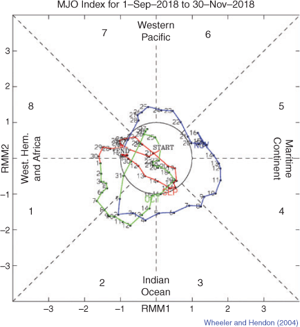
The MJO is a tropical convective wave anomaly which develops in the Indian Ocean and propagates eastwards into the Pacific Ocean (Madden and Julian 1971, 1972, 1994). The MJO takes approximately 30 to 60 days to reach the western Pacific, with a frequency of six to twelve events per year (Donald et al. 2004). When the MJO is in an active phase, it is associated with areas of increased and decreased tropical convection, with effects on the southern hemisphere often weakening during early autumn, before transitioning to the northern hemisphere. A description of the Real-time Multivariate MJO (RMM) index and the associated phases can be found in Wheeler and Hendon (2004).
The phase-space diagram of the RMM for spring 2018 is shown in Fig. 6. The MJO was relatively inactive during September and October, apart from a brief period of activity in the western Indian Ocean in the first half of October, which was associated with the development of Cyclone Luban in the Arabian Sea. A high level of MJO activity then occurred for most of November. This led to increased convection in the Indian Ocean in early November and the development of the first major southern hemisphere tropical cyclone of the season, Cyclone Alcide, which reached a peak intensity of 90-knot sustained winds on 8 November east of the northern tip of Madagascar. By mid-November the MJO was centred in the Maritime Continent region, contributing to heavy early-season rains in the third week of November in the Top End of the Northern Territory.
|
5 Oceanic patterns
5.1 Sea surface temperatures (SSTs)
The SST for the combined ocean area of the southern hemisphere for spring 2018 was 0.64°C above the 20th century average,8 the second-highest on record after 2015. The western equatorial Pacific was particularly warm (Fig. 7), with most areas west of 150°W being 1°C or more above average. More localised anomalies on this scale also occurred in the equatorial central and eastern Pacific, consistent with Pacific conditions approaching El Niño levels, and in the western equatorial Indian Ocean, consistent with a positive phase of the IOD. Anomalies exceeding +1°C were also found east of New Zealand, off the subtropical east coast of South America, south of South Africa and in the central Indian Ocean near 30°S, 80°E. Most of the South Pacific north of 45°S was at least 0.5°C above average, as was the western half of the Indian Ocean.

|
The SSTs in the Australian region are shown in Fig. 8. Although they were relatively warm around most parts of the continent, one notable feature was the relatively cool area off the coast of Western Australia, one of the relatively few southern hemisphere regions with below-average SSTs. Temperatures were near average off the Indonesian coast in the eastern node of the IOD. Over the Australian region,9 SSTs for spring were 0.36°C above the 1961–1990 average, the 16th highest in the post-1900 period, but the lowest since 2008 and 0.41°C below the spring record set in 2010. The Tasman Sea was the fifth-warmest on record (although still cooler than 2016 and 2017) and the Coral Sea sixth-warmest. The Southwest region was only 0.08°C above the 1961–1990 average, the equal-lowest since 2005.

|
5.2 Equatorial subsurface patterns
The 20°C isotherm depth is generally located close to the equatorial thermocline, which is the region of greatest temperature gradient with depth and is the boundary between the warm near-surface and cold deep-ocean waters. Therefore, measurements of the 20°C isotherm depth make a good proxy for the thermocline depth. Negative anomalies correspond to the 20°C isotherm being shallower than average and is indicative of a cooling of subsurface temperatures. If the thermocline anomaly is positive the depth of the thermocline is deeper. A deeper thermocline results in less cold water available for upwelling, and therefore a warming of surface temperatures (Fig. 9).

|
Warm subsurface waters were present through much of the equatorial Pacific during spring 2018, reaching their greatest extent and intensity in October when they covered almost the full width of the Pacific, with peak anomalies around +4°C near 130°W (Fig. 10). In November the warm anomalies weakened slightly and became more focused in the eastern half of the Pacific. The 20°C isotherm was also deeper than normal in October and November (Fig. 9), especially east of 140°W. Warm anomalies in this region are consistent with developing El Niño or near-El Niño conditions.

|
6 Antarctic
6.1 Sea ice
The seasonal sea ice extent maximum was reached on 2 October,10 slightly later than the climatological median. The maximum extent in 2018 was 18.15 million km2, slightly above that of 2017 but still the fourth-lowest in the (post-1979) satellite record. The most prominent areas of below-average sea ice extent were in the Bellinghausen and Amundsen Seas, south of Australia and south of Africa.
Sea ice extent was most anomalously low early in the spring, with a brief decline in mid-September (at a time when it would normally be expanding) taking it to near-record low levels for the date, before a slight recovery to the early October peak. The decline of sea ice extent during November was slower than usual, but extent was still well below the post-1979 average at the end of spring, although well above the record low late spring levels of 2016.
6.2 Ozone
The Antarctic ozone hole typically forms in August and breaks down in late November or early December. The 2018 ozone hole was relatively large and deep compared with recent years. The maximum ozone hole size was 24.7 million km2 on 20 September, and the 15-day maximum was 24.1 million km2 (Krummel et al. 2019). This ranks 14th highest of the post-1979 period and slightly above the 2009–2018 mean of 22.6 million km2, and was larger than 2016 or 2017, although smaller than 2015. The minimum ozone level reached was 102 Dobson Units on 11 and 12 October, ranking as 13th deepest of the last 40 years. The ozone hole broke down on 3 December, close to the median date. A contributor to the relatively large ozone hole was a relatively stable Antarctic circulation, reflected in low stratospheric temperatures. Temperatures at the 50 hPa and 100 hPa levels, averaged over the region south of 60°S, were below average for most of the spring.
7 Atmospheric circulation
7.1 Southern Annular Mode (SAM)
The SAM index11 was positive in all three months of spring 2018. The seasonal mean value of the CPC index was +0.99, the highest for spring since 2010. The only period where negative values were sustained for more than a few days was in mid-October. Particularly strong positive values occurred in the first 10 days of September, with daily values exceeding +4 at times. The wet conditions in coastal New South Wales in late spring, and dry conditions further west in Victoria and Tasmania, were consistent with the generally positive SAM.
7.2 Surface analyses
The MSLP pattern for spring 2018 is shown in Fig. 11, computed using data from the 0000 UTC daily analyses of the Bureau of Meteorology’s Australian Community Climate and Earth System Simulator (ACCESS) model.12 MSLP anomalies are shown in Fig. 12, relative to the 1979–2000 climatology obtained from the National Center for Environmental Prediction (NCEP) II Reanalysis data (Kanamitsu et al. 2002). The MSLP anomaly field is not shown over areas of elevated topography (grey shading).

|

|
Consistent with the positive seasonal SAM, MSLP was above average over most areas between 30°S and 55°S, except for the eastern Pacific, and below average over most areas south of 55°S. Seasonal MSLP anomalies were not exceptionally large with the largest positive anomalies, between 4 and 5 hPa, over the central Indian Ocean centred near 45°S, 80°E, and near the South Island of New Zealand. Positive MSLP anomalies extended north to cover all of Australia and the Maritime Continent. The largest negative MSLP anomalies were near the Antarctic coast, with values reaching −8 hPa over the Ross Sea, as well as near 90°E.
7.3 Mid-tropospheric analyses
The 500-hPa geopotential height, an indicator of the steering of surface synoptic systems across the southern hemisphere, is shown for spring 2018 in Fig. 13. The associated anomalies are shown in Fig. 14.

|

|
Geopotential height is valuable for identifying and locating features like troughs and ridges, which are the upper-level equivalents of surface low and high pressure systems respectively. In spring 2018, broad hemispheric patterns at the 500-hPa level were similar to those at the surface, with positive geopotential height anomalies in most areas between 30°S and 55°S and negative anomalies further south. Also similar to the surface pattern, the largest anomalies were in the central Indian Ocean and near New Zealand. There was a long-wave trough centred near 120°E south of Western Australia, and weaker troughs existed in the eastern South Pacific and central South Atlantic.
8 Winds
Figs 15 and 16 show spring 2018 low-level (850 hPa) and upper-level (200 hPa) wind anomalies respectively (winds computed from ACCESS and anomalies with respect to the 22-year 1979–2000 NCEP climatology). Isotach contours are at an interval of 5 ms−1.

|

|
At lower levels, the most notable anomaly was enhanced westerly flow over a belt centred on about 50–60°S, consistent with the enhanced pressure gradient over the region, with anomalously strong high pressure to the north and low pressure to the south. These anomalies were especially pronounced in the Indian Ocean, south of Australia and in the western South Pacific. Anomalous easterly flow was observed in the Tasman Sea, and in the subtropical Indian Ocean west of Australia. Despite the near-El Niño conditions that developed during the season, winds in the southern hemisphere tropics were close to normal, with westerly anomalies in the Pacific largely confined to areas north of the Equator.
At upper levels, the subtropical jet in the South Pacific was stronger than normal, with westerly anomalies at 200 hPa extending almost across the ocean, as well as across South America and into the western Atlantic. The strongest anomalies were west of the South American coast. Westerly anomalies also occurred around 55–60°S over large parts of the Indian and Pacific Ocean sectors. The 200-hPa wind anomalies in the southern hemisphere tropics were generally weak except for north-westerly anomalies near and off the east coast of Africa.
9 Australian region
9.1 Rainfall
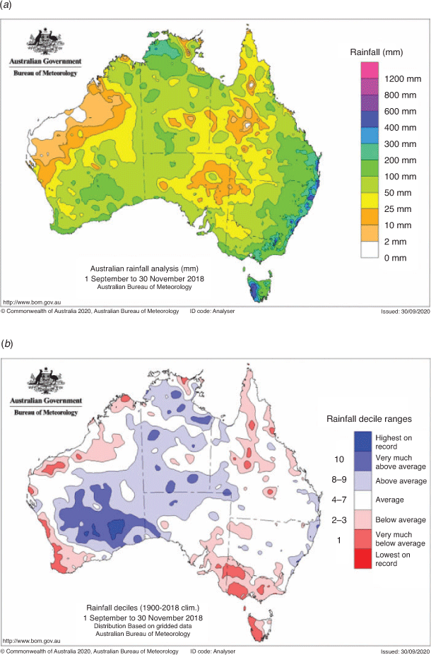
Rainfall averaged over Australia in spring 2018 was near average. September was the driest on record nationally with average rainfall of 5.3 mm, breaking the record of 5.6 mm set in 1957, but October and November were both slightly wetter than normal, following a very dry period from April to September.
Relatively few regions had spring rainfall either well above or well below average (Fig. 17). The most significant area of above-average rainfall was in the southern interior of Western Australia, extending east into the Nullarbor. There were a number of widespread rain events in this region in early October and in the first half of November. In contrast, the southwest of Western Australia was relatively dry, with areas of very much below rainfall on and near the west coast.
|
October and November rainfall totals were sufficient to offset the dry September in both New South Wales and Queensland, with the majority of both states having seasonal rainfall close to average. Heavy rain fell in coastal areas of southern Queensland and northern New South Wales in mid-October, and southern New South Wales at the end of November. Victoria and Tasmania both had dry springs (Table 1), with rainfall very much below average in most of the western half of Victoria and western Tasmania. Early wet season rains were generally close to average in the northern tropics.

|
Rainfall analyses in this summary use the Australian Water Availability Project data set (Jones et al. 2009).
9.2 Rainfall deficiencies
Rainfall deficiencies persisted at a range of timescales over much of the southeast quarter of mainland Australia. For the second successive year, the April to September period was significantly drier than usual over most of the Murray-Darling Basin, as well as in most remaining areas of Queensland and New South Wales, and southern Victoria from Melbourne eastwards (Table 2).

|
Rain during October and November cleared most rainfall deficiencies on the east coast and in the southeast quarter of Queensland, and moderated conditions somewhat in eastern inland New South Wales. Severe rainfall deficiencies persisted, however, in much of the western half of New South Wales, especially the northwest quarter (Fig. 18), as well as in the Victorian and South Australian Mallee and adjacent parts of far southwest New South Wales. Another significant area of persistent severe rainfall deficiencies was central and east Gippsland in Victoria.

|
9.3 Temperature
Spring 2018 was warm with above-average maximum and minimum temperatures across most of the continent (Tables 3–5). Although it was not as hot as some recent springs, mean temperatures were still 1.21°C above the 1961−1990 average. For 2002–2018, 12 of the 17 springs have been at least 1°C above average, a threshold that had only been reached once (in 1980) prior to 2000. All three months were warmer than average, with October the most significantly above normal.

|

|

|
The most abnormal maximum temperatures occurred in tropical Australia (Fig. 19). All three of Western Australia, the Northern Territory and Queensland had tropical regions where spring mean maximum temperatures were the highest on record (Table 5). An extreme heatwave affected eastern Queensland in the last week of November (Bureau of Meteorology 2018). Numerous locations had their highest temperature on record, including Cooktown, Cairns Airport, Innisfail, Bowen and Proserpine. The extreme heat, and the dry westerly winds that accompanied it, contributed to significant bushfires in many parts of eastern Queensland (Lewis et al. 2020). Almost all of tropical Queensland and the Northern Territory had maximum temperatures very much above average, along with the Kimberley in Western Australia. Another small area of very much above average maximum temperatures straddled the New South Wales–Victorian border. The only area with below-average maximum temperatures was a small area around Carnarvon on the west coast.

|
Minimum temperatures were also above average in most regions (Fig. 20), and very much above average in most of New South Wales, Queensland and the Northern Territory, as well as in parts of southern Victoria and Tasmania. They were the warmest on record in parts of northeast New South Wales. September average minimum temperatures were the lowest on record, with numerous and sometimes damaging late-season frosts, in much of northern Victoria and eastern South Australia, with statewide averages for the month for South Australia and Victoria being the lowest since 1985 and 1994 respectively. However, this was largely offset in seasonal averages by warm conditions in October and November, with only a few localised areas in South Australia between Adelaide and the Victorian border having below-average temperatures for the season as a whole.

|
10 Southern hemisphere
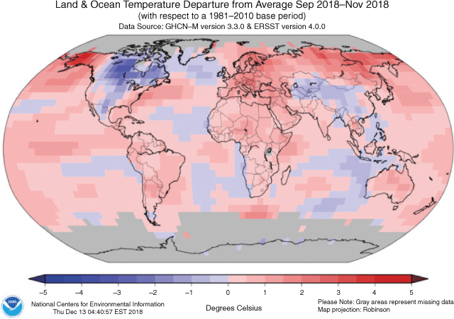
Temperatures were well above the long-term average over the southern hemisphere in spring 2018. Almost all land areas outside the Antarctic had seasonal mean temperatures near or above the 1981–2010 average, with the only significant cool SST anomalies being in the eastern Indian Ocean. It was the second-warmest spring on record for the southern hemisphere, after 2015, in the NOAA (Huang et al. 2020) and GISS (Lenssen et al. 2019) data sets, and third-warmest in the HadCRUT4 data set (Morice et al. 2012).
The strongest warm anomalies, more than 1°C above the 1981–2010 average, were in eastern Australia and the northern half of Argentina (Fig. 21). September was especially warm in Argentina, with several northern provinces having their warmest September on record. Spring temperatures were generally slightly above average in southern Africa, and near average in New Zealand. All three Australian Antarctic bases had spring temperatures about 0.5°C below average, but many other parts of Antarctica had above-average temperatures, including the South Pole, the Antarctic Peninsula and the Ross Sea area.
|
Southern Africa had a generally dry spring, with most areas receiving spring rainfall between 40% and 80% below average (Fig. 22). This contributed to an intensification of drought affecting many parts of the region. The “short rains” season of October–November in equatorial East Africa was also drier than average. Most of South America east of the Andes had above-average rainfall for the season with seasonal anomalies widely in the range from 20% to 60%, while spring rainfall was below average around Santiago in Chile, but near to above average in many areas further south. In New Zealand, spring rainfall was generally above average on the east side of both islands, particularly the eastern South Island which experienced flooding in November, and below average on the west coast.

|
Conflicts of interest
The author declares no conflict of interest.
Acknowledgements
The comments of Ben Hague and Robert Fawcett are gratefully acknowledged. This research did not receive any specific funding.
References
Bureau of Meteorology, (2018). An extreme heatwave on the tropical Queensland coast. Special Climate Statement 67, Bureau of Meteorology, Melbourne. Available at http://www.bom.gov.au/climate/current/statements/scs67.pdf.Chapman, B., and Rosemond, K. (2020). Seasonal climate summary for the southern hemisphere (autumn 2018): a weak La Niña fades, the austral autumn remains warmer and drier. J. South. Hemisph. Earth Sys. Sci. , .
| Seasonal climate summary for the southern hemisphere (autumn 2018): a weak La Niña fades, the austral autumn remains warmer and drier.Crossref | GoogleScholarGoogle Scholar |
Donald, A., Meinke, H., Power, B., Wheeler, M. and Ribbe, J. (2004). Forecasting with the Madden-Julian Oscillation and the applications for risk management. Brisbane, 4th International Crop Science Congress, 2004.
Huang, B., Thorne, P. W., Banzon, V. F., et al. (2017). Extended Reconstruction Sea Surface Temperature, Version 5 (ERSSTv5): upgrades, validations and intercomparisons. J. Climate 30, 8179–8205.
| Extended Reconstruction Sea Surface Temperature, Version 5 (ERSSTv5): upgrades, validations and intercomparisons.Crossref | GoogleScholarGoogle Scholar |
Huang, B., Menne, M. J., Boyer, T., et al. (2020). Uncertainty estimates for sea surface temperatures and land surface air temperatures in NOAAGlobalTemp version 5. J. Climate 33, 1351–1379.
| Uncertainty estimates for sea surface temperatures and land surface air temperatures in NOAAGlobalTemp version 5.Crossref | GoogleScholarGoogle Scholar |
Jones, D. A., Wang, W., and Fawcett, R. (2009). High-quality spatial climate data-sets for Australia. Aust. Met. Oceanogr. J. 58, 233–248.
| High-quality spatial climate data-sets for Australia.Crossref | GoogleScholarGoogle Scholar |
Kanamitsu, M., Ebisuzaki, W., Woollen, J., Yang, S.-K, Hnilo, J. J., Fiorino, M., and Potter, G. L. (2002). NCEP-DOE AMIPII Reanalysis (R-2). Bull. Amer. Met. Soc. 83, 1631–1643.
| NCEP-DOE AMIPII Reanalysis (R-2).Crossref | GoogleScholarGoogle Scholar |
Krummel, P. B., Fraser, P. J. and Derek, N. (2019). The 2018 Antarctic Ozone Hole Summary: Final Report. Report prepared for the Australian Government Department of the Environment and Energy, CSIRO, Australia.
Kuleshov, Y., Qi, L., Fawcett, R., and Jones, D. (2009). Improving preparedness to natural hazards: Tropical cyclone prediction for the Southern Hemisphere. Adv. Geosci. 12, 127–143.
Lenssen, N. J. L., Schmidt, G. A., Hansen, J. E., Menne, M. J., Persin, A., Ruedy, R., and Zyss, D. (2019). Improvements in the GISTEMP uncertainty model. J. Geophys. Res. Atmos. 124, 6307–6326.
| Improvements in the GISTEMP uncertainty model.Crossref | GoogleScholarGoogle Scholar |
Lewis, S. C., Blake, S. A. P., Trewin, B., Black, M. T., Dowdy, A. J., Perkins-Kirkpatrick, S. E., King, A. D., and Sharples, J. J. (2020). Deconstructing factors leading to the 2018 fire weather in Queensland, Australia. Bull. Amer. Met. Soc. 100, S115–S123.
| Deconstructing factors leading to the 2018 fire weather in Queensland, Australia.Crossref | GoogleScholarGoogle Scholar |
Madden, R. A., and Julian, P. R. (1971). Detection of a 40-50 day oscillation in the zonal wind in the tropical Pacific. J. Atmos. Sci. 28, 702–708.
| Detection of a 40-50 day oscillation in the zonal wind in the tropical Pacific.Crossref | GoogleScholarGoogle Scholar |
Madden, R. A., and Julian, P. R. (1972). Description of global-scale circulation cells in the tropics with a 40-50 day period. J. Atmos. Sci. 29, 1109–1123.
| Description of global-scale circulation cells in the tropics with a 40-50 day period.Crossref | GoogleScholarGoogle Scholar |
Madden, R. A., and Julian, P. R. (1994). Observations of the 40-50 day tropical oscillation: a review. Mon. Wea. Rev. 122, 814–837.
| Observations of the 40-50 day tropical oscillation: a review.Crossref | GoogleScholarGoogle Scholar |
Meyers, G., McIntosh, P., Pigot, L., and Pook, M. (2007). The years of El Niño, La Niña, and interactions with the tropical Indian Ocean. J. Climate 20, 2872–2880.
| The years of El Niño, La Niña, and interactions with the tropical Indian Ocean.Crossref | GoogleScholarGoogle Scholar |
Morice, C. P., Kennedy, J. J., Rayner, N. A., and Jones, P. D. (2012). Quantifying uncertainties in global and regional temperature change using an ensemble of observational estimates: the HadCRUT4 dataset. J. Geophys. Res. 117, D08101.
| Quantifying uncertainties in global and regional temperature change using an ensemble of observational estimates: the HadCRUT4 dataset.Crossref | GoogleScholarGoogle Scholar |
Troup, A. (1965). The Southern Oscillation. Quart. J. Roy. Meteor. Soc. 91, 490–506.
| The Southern Oscillation.Crossref | GoogleScholarGoogle Scholar |
Ummenhofer, C. C., England, M. H., McIntosh, P. C., Meyers, G. A., Pook, M. J., Risbey, J. S., Sen Gupta, A., and Taschetto, A. S. (2009). What causes southeast Australia’s worst droughts?. Geophys. Res. Lett. 36, L04706.
| What causes southeast Australia’s worst droughts?.Crossref | GoogleScholarGoogle Scholar |
Wang, G., and Hendon, H. (2007). Sensitivity of Australian rainfall to inter-El Niño variations. J. Climate 20, 4211–4226.
| Sensitivity of Australian rainfall to inter-El Niño variations.Crossref | GoogleScholarGoogle Scholar |
Wang, X., and Wang, C. (2014). Different impacts of various El Niño events on the Indian Ocean Dipole. Clim. Dyn. 42, 991–1015.
| Different impacts of various El Niño events on the Indian Ocean Dipole.Crossref | GoogleScholarGoogle Scholar |
Wheeler, M., and Hendon, H. (2004). An All-Season Real-Time Multivariate MJO Index: Development of an Index for Monitoring and Prediction. Mon. Wea. Rev. 132, 1917–1932.
| An All-Season Real-Time Multivariate MJO Index: Development of an Index for Monitoring and Prediction.Crossref | GoogleScholarGoogle Scholar |
Wolter, K., and Timlin, M. S. (2011). El Niño/Southern Oscillation behaviour since 1871 as diagnosed in an extended multivariate ENSO index (MEI.ext). Int. J. Climatol. 31, 1074–1087.
| El Niño/Southern Oscillation behaviour since 1871 as diagnosed in an extended multivariate ENSO index (MEI.ext).Crossref | GoogleScholarGoogle Scholar |
1 The Troup SOI (Troup, 1965) used in this article is 10 times the standardised monthly anomaly of the difference in mean sea level pressure (MSLP) between Tahiti and Darwin. The calculation is based on 60-year climatology (1933–1992), with records commencing in 1876. The Darwin MSLP is provided by the Bureau of Meteorology, and the Tahiti MSLP is provided by Météo France inter-regional direction for French Polynesia.
2 ENSO 5VAR was developed by the Bureau of Meteorology and is described in Kuleshov et al. (2009). The principal component analysis and standardisation of this ENSO index is performed over the period 1950–1999.
3 SST indices obtained from ftp://ftp.cpc.ncep.noaa.gov/wd52dg/data/indices/sstoi.indices.
4 The standardised MEIv2 was obtained from https://psl.noaa.gov/enso/mei/.
5 http://www.bom.gov.au/climate/iod/.
6 http://www.bom.gov.au/climate/iod/#tabs=Pacific-Ocean-interaction.
7 Standardised monthly OLR anomaly data obtained from http://www.cpc.ncep.noaa.gov/data/indices/olr.
8 NOAA National Centers for Environmental information, Climate at a Glance: Global Time Series, from http://www.ncdc.noaa.gov/cag/(base period 1901–2000).
9 The Australian region is defined here as 4–46°S, 94–174°E. Sub-regional boundaries are available at http://www.bom.gov.au/climate/change/about/sst_timeseries.shtml.
10 Sea ice information from the National Snow and Ice Data Center. http://www.nsidc.org.
11 For more information on the SAM index from the Climate Prediction Center (NOAA), see http://www.cpc.ncep.noaa.gov/products/precip/CWlink/daily_ao_index/aao/aao.shtml.
12 For more information on the Bureau of Meteorology’s ACCESS model, see http://www.bom.gov.au/nwp/doc/access/NWPData.shtml.
13 A subset of the full temperature network is used to calculate the spatial averages and rankings shown in Table 3 (maximum temperature), Table 4 (minimum temperature) and Table 5; this dataset is known as ACORN-SAT (see http://www.bom.gov.au/climate/change/acorn-sat/for details). These averages are available from 1910 to the present. As the anomaly averages in the tables are only retained to two decimal places, tied rankings are possible.