
Cutoff low over the southeastern Pacific Ocean: a case study
Nelson Quispe-Gutiérrez A B , Vannia Aliaga-Nestares A , Diego Rodríguez-Zimmermann A , Martí Bonshoms A , Raquel Loayza A , Teresa García A , José Mesia A , Ricardo Duran A and Sara Olivares AA Servicio Nacional de Meteorología e Hidrología (SENAMHI), Jr. Cahuide 785 Jesús María, Lima – Perú.
B Corresponding author. Email: nquispe@senamhi.gob.pe
Journal of Southern Hemisphere Earth Systems Science 71(1) 17-29 https://doi.org/10.1071/ES19051
Submitted: 14 April 2020 Accepted: 19 11 2020 Published: 17 February 2021
Journal Compilation © BoM 2021 Open Access CC BY-NC-ND
Abstract
Cutoff lows (COLs) are infrequent events in the tropics that can cause extreme rainfall, flash flooding and landslides in arid areas, such as western South America. In this study, the life cycle of a COL in the southeastern Pacific at the beginning of April 2012 was analysed using the ERA-Interim reanalysis dataset. This paper examines: (1) the precursor flow evolution prior to the COL, its development and dissipation by applying the quasi-geostrophic and vorticity equations; and (2) the influence of the COL in the heavy precipitation events over the western Peruvian Andes. During April 2012, the highest amount of precipitation was recorded in Chosica (850 masl) with 37 mm on 5 April. Days prior to the formation of the COL, a subtropical trough deepened by the amplification of a ridge over the tropical Pacific and the incursion of cold air from medium and low levels into the trough. The strong cyclonic vorticity advection was intensified by a short-wave trough embedded inside a long-wave one that strengthened the system on 5 April 2012. In the dissipation stage, warm vertical advection predominated, resulting in the reabsorption of the COL by a new trough. Understanding the behaviour COL systems is important for reducing the impact of these extreme weather events on lives and infrastructure in densely populated areas.
Keywords: Andes cordillera, Chosica, Cutoff low, extreme rainfall, Peru, quasi-geostrophic equations, ridge-trough, southeastern Pacific.
1 Introduction
A segregated low, also known as a cutoff low (COL), is a synoptic system with a cold core that develops in the high troposphere. COLs were studied initially by Palmén (1949) and Palmer (1951), who acknowledged the existence of a cold centre with different thermodynamic characteristics according to the area of its formation. In the southeast Pacific, the COLs progress to the east is disturbed by the Andes cordillera, which reduces their propagation speed and deflects their trajectory to the south.
In southern South America, Godoy et al. (2011) found that, at high levels, the trough begins to seclude itself from the main western flow during the COL’s formation stage. Meanwhile, Campetella and Possia (2007) demonstrated that, during the segregation stage, the strong cold advection in lower levels over the eastern flank of the associated migratory anticyclone contributes to the deepening of this trough. Then, the amplification of a ridge and propagation of a short-wave trough associated with a strong cyclonic potential vorticity in high troposphere drives the segregation process from their polar source (Bell and Bosart 1993). While fully developed, the system is independent of the main western flow, observing an isolated cyclonic vortex in high and medium levels and a warm core over it, related to the lowering of the tropopause and the presence of fronts in high troposphere (Hoskins et al. 1985; Rondanelli et al. 2002). Both Garreaud and Fuenzalida (2007) and Quispe and Avalos (2006), explained that the intensification of the COL can be attributed to the amplification and growth of the ridge that follows. Finally, in the dissipation stage, warm vertical advection dominates (Godoy et al. 2011), which contributes to the demise of the system.
According to Pinheiro (2010), the formation of COLs over the Pacific Ocean is related to the presence of stationary Rossby waves. As a result, the majority are observed off the central coast of Chile (Fuenzalida et al. 2005; Campetella and Possia 2007). The interest in studying COLs located east of South America lies in the impact they have on precipitation on the arid coast and western Andean cordillera. In Peru, episodes of severe weather (hail, heavy rainfall and snowfall) during the dry season are associated with these systems. Quispe and Avalos (2006) analysed the effects of a COL over the Pacific Ocean in the winter of 2004, which generated intense solid precipitation in the Peruvian high plateau (3800–4000 masl), affecting livestock and the health of the population (INDECI 2004).
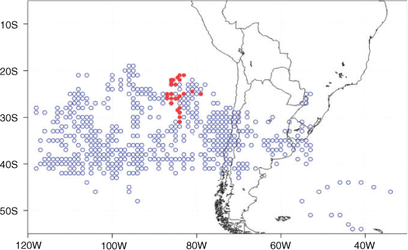
In early April 2012, moderate to heavy precipitation occurred throughout the western side of the Peruvian Andes, with anomalies of over 100% in many areas and some exceeding 300% in the central and southern regions (Fig. 1). The precipitation events caused flash floods that affected the arid western Peruvian Andes. One of the highest anomalies was recorded in Chosica (850 masl) in the Rímac river valley. This district, located in an arid region, has an annual average rainfall of 8.4 mm, but during the afternoon of 5 April 2012, it registered rainfall of roughly 33 mm in just 2 h, with a 37 mm record at the end of the day. Meanwhile, the monthly average (1989–2010) for April is 0.9 mm. The occurrence of flash floods and landslides (also known as ‘huaycos’) in the rocky and arid slopes of the surrounding mountains resulted in 1607 victims (29 wounded, 2 dead), 569 collapsed houses, 1 damaged educational institution and problems in the communication routes of the district (INDECI 2012).

|
Knowing this, our study examines the life cycle and displacement of this COL and its consequences during the first 10 days of April 2012, when heavy rainfall and flash floods affected the arid western Peruvian Andes, which can be observed in the distribution of daily precipitation of the weather stations in Fig. 1.
2 Data and methodology
The study area extends from 40°S–120°W up to 0°–60°W, including the subtropical sector of the southeastern Pacific, as well as Peru. Data from the ERA-Interim reanalysis (Dee et al. 2011) has been used; this reanalysis has a grid spacing of 79 km (~0.75°), a temporal resolution of 6 h and 37 pressure levels (from 1000 to 10 hPa). The information includes data between 1 and 10 April 2012.
For the identification of the COL, we chose the following characteristics: a closed core of at least 1.6 potential vorticity units (PVU; 1 PVU = 10−6 m2 s−1 K kg−1) at 300 hPa and a closed cyclonic nucleus with a 30 gpm interval at 500 hPa.
To analyse the trajectory of air masses before the occurrence of the event, the National Oceanic and Atmospheric Administration’s Hybrid Single Particle Lagrangian Integrated Trajectory (HYSPLIT) model was used. The model calculation method is a hybrid between the Lagrangian approach that calculates the trajectories of air parcels from their initial location and the Eulerian methodology (Stein et al. 2015). The model is available for download at https://ready.arl.noaa.gov/HYSPLIT.php. We simulated 120 h of backward air trajectories before the severe precipitation event in Chosica with a height between 500 and 3000 masl using meteorological fields for the Chosica basin from the ERA-Interim reanalysis dataset. The levels studied are within the cloud formation layer during the precipitation event, and therefore, they are used as a proxy for moisture transport at low and medium altitudes.
For the analysis of the event, daily precipitation data (from 12:00Z to 12:00Z of April 2012) we used 151 conventional weather stations belonging to the network of the National Service of Meteorology and Hydrology of Peru (SENAMHI) and located in the western fringe of the cordillera (Fig. 1). The weather station of Chosica appears among stations where the climatological average of April was exceeded in the first 10 days. The precipitation of Chosica is compared with its monthly average and with the daily maximum of the entire series; an automatic weather station near the area is also considered.
For the determination of the potential vorticity (PV), finite differences between the upper and lower level were used (Z − 1 and Z + 1 hPa) at a given isobaric level, identifying the dynamic tropopause with values of –1.6 PVU (PVU = m2 s−1 K kg−1) (WMO 1986).
For the calculations of the PV, the equation exposed by Hoskins (1985), which defines the isentropic PV, was used:
where ζ is the relative vorticity, f is the Coriolis parameter, g is the acceleration of gravity, P is the pressure, ∇p is the horizontal gradient of the isobaric surface, V is the horizontal wind vector and θ is the potential temperature.
Bell and Bosart (1993) presented the isentropic PV formula in isobaric coordinates as follows:
For the quasi-geostrophic analysis, the geopotential trend equation solved by Holton (2004) was considered and stated as follows:
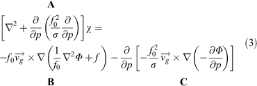
This equation provides the relationship between the local geopotential tendency (term A), the vorticity advection distribution (term B) and the thickness advection (term C).
3 COLs in the Pacific
As seen in Fig. 2, the climatology of COLs for the month of April over the southern Pacific (between 1948 and 2010) shows a disperse area between 49°S and 18°S, with a concentration between 30°S and 40°S. The COL in early April 2012 had its centre between 30°S and 20°S, reaching the northernmost position further north than previous COLs, even when compared with the March-April-May climatology obtained by Fuenzalida et al. (2005).
|
4 Circulation patterns during the event
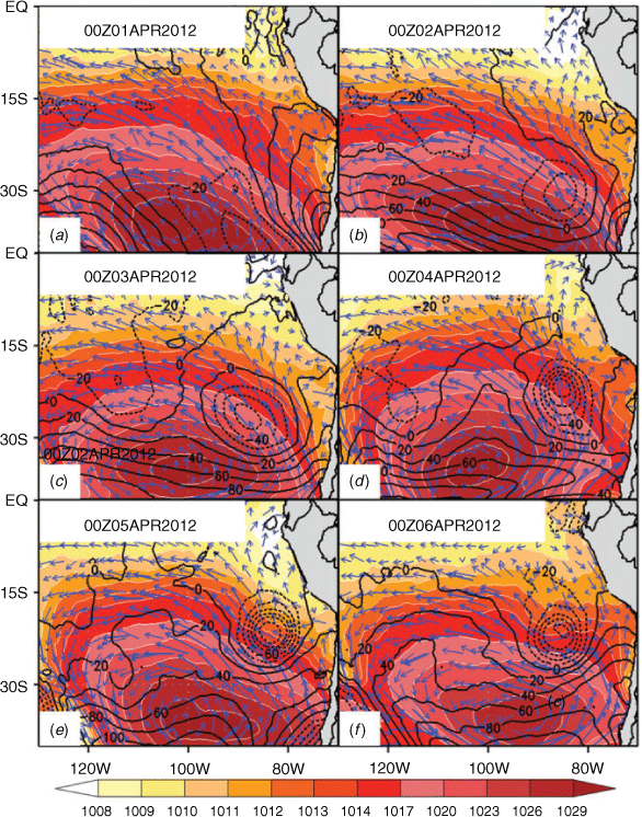
At higher levels, the Polar Jet (PJ) accompanied a very faint ridge over 45°S and a trough towards the northwest, initially located at 80°W 35°S (approximately) at 00:00 UTC on 2 April (Fig. 3a), showing an anticyclonic wave breaking (Thorncroft et al. 1993). The jet continues its trajectory off the coast of Chile along a very pronounced ridge traveling towards higher latitudes north of the trough in front of it. The latter finally becomes a closed cyclonic system with a core located at 85°W 25°S. By 00:00 UTC on 6 April, the system was close to the central Peruvian coast, increasing the western wind speed. Over South America, the Bolivian High (BH) was well defined (65°W 12°S), with an intense core located slightly to the north of its normal position. The pressure gradient caused by the BH, results in a wind speed increase and, consequently, an increase of divergence in the centre-south sector of Peru, with flows from the east supporting moisture transport to the western Andes (Fig. 3b). Subsequently, in the dissipation stage, the COL weakened and moved towards the southeast, being reabsorbed by the western flow off the coast of Chile at about 40°S (Fig. 3c).

|
At 500 hPa, a pattern very similar to 200 hPa is observed, with a deep trough of inclined axis towards the northwest, between 80°W and 90°W, with a core of maximum cyclonic vorticity between 25°S and 30°S (Fig. 4a). This trough travelled north with help from the intense ridge to its west, which tended to move towards higher latitudes (Fig. 4b). On 4 April (Fig. 4c) the COL started separating from the trough. Between the ridge and the trough, the presence of a short wave is observed at 90°W 35°S, which is later absorbed by the COL, intensifying it in the maturity stage (Figs 4a and 4c). The trough entered the continent on 6 April, driven by the intense western flow associated with the PJ and the amplification of the ridge, leaving the vortex of the trough lagging behind and isolating its core (Fig. 4d).
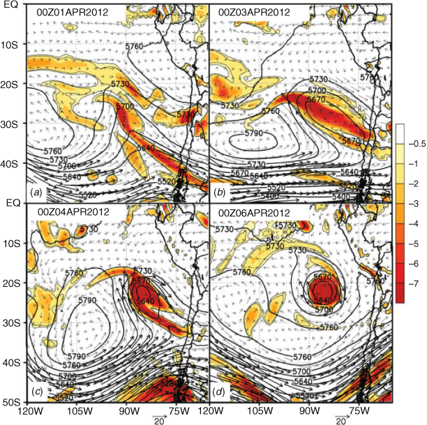
|
In the formation stage between 1 and 2 April (Figs 5a and 5b), the cold core shows a negative anomaly of 40 m, centred at 32.5°S 85°W (Fig. 5b), while the isobaric field shows the presence of the South Pacific Anticyclone, with 1029 hPa at its centre, at 35°S 95°W. On 3 April (Fig. 5c), the cold core is already enclosed with a negative anomaly of 60 m and slightly north of its initial position, moving towards the north on 4 April (Fig. 5d).
|
On 5 April, the most system development occurred (Fig. 5e). The COL was in the stage of maturity (Godoy et al. 2011), presenting a negative anomaly of 120 m at 22.5°S 83°W, a further northeast position and a slight cyclonic perturbation of the isobaric field. By 6 April, the heavy precipitation event in Chosica occurred and the COL decreased its intensity (Fig. 5f). The system reached lower levels and fused with an inverted coastal trough, changing the coastal winds from southerlies on 2 April to northerlies on 5 April, which transported hot and humid air from equatorial latitudes towards the Peruvian coast and cold air to the west of the system.
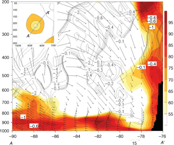
In Fig. 6, the cross section is denoted from the southwest end of the COL to the northeast end over Chosica at 18:00 UTC, just before the beginning of the precipitation event, which occurred between 21:00 and 23:00 UTC. The gradual displacement of the COL towards the northeast induced the change in direction of the trade winds in the lower levels from southeast to northwest off the Peruvian coast (Fig. 5), a physical characteristic which is not typical of the trade winds. This northern flow carried warm and humid air, confining the humidity on to the central coast of Peru. Likewise, the circulation at higher levels (Fig. 6) denotes the influence of the COL, which promoted cyclonic vorticity advection towards the coast, the rise of humid air towards higher levels and a rapid state of saturation in the atmospheric column. Other characteristics observed were convergence at lower levels and strong divergence at higher levels, a condition that favoured the occurrence of the unusual precipitation in Chosica.
|
The moisture flux at medium levels during the maturity stage of the COL (Figs 7a and 7b), intensified towards the central and southern sector of the cordillera, favouring the moisture transfer from the Amazon basin towards the western Andes. The presence of the cyclonic vortex in front of the Gulf of Arica generated an increase in the mixing ratio flux (above its average) with an east-northeast anomaly component, which favoured intense rainfall in the Andean cordillera.

|
The result of the HYSPLIT model analysis of the 120 h backward trajectories for the precipitation event in Chosica suggests two main sources of moisture: (1) from the Amazon basin and (2) from the western slope of the Andes (Fig. 7c). The former has a stronger contribution of humidity in the wet season, while the latter is more sporadic, occurring only when a coastal northern flow is present, as shown in Figs 5 and 6. The heavy precipitation in Chosica is particularly surprising, since the behaviour of precipitation on the western slope of the Andes, especially along the coast, is affected by subsidence (Wood 2012), causing stratocumulus to predominate throughout the southeastern Pacific. However, the presence of the COL led to the occurrence of atypical physical properties over the study area: a downward flow from higher altitudes from the Amazon reached Chosica and then rose due to convection and, at the same time, the coastal northern flow transported humidity that converged in the western side with divergence at higher levels (figure not shown).
5 Potential vorticity analysis
The accepted criterion for the identification of a COL, used by Hoskins et al. (1985); Hoskins (1991) and Van Delden and Neggers (2003) consists of identifying a closed cyclonic core at 500 hPa with intervals of 30 m. In addition to this step, a 1.6 PVU threshold at the 300 hPa level was added (WMO 1986).
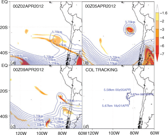
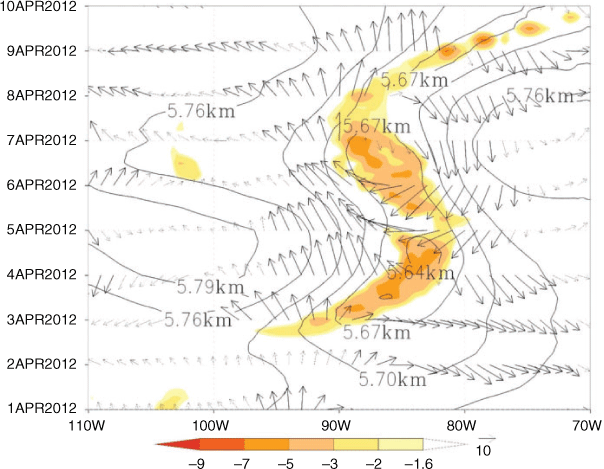
Following this methodology, the COL can be observed on 2 April at 00:00 UTC with a core of 5670 m. The core travelled towards the northeast, reaching a minimum latitude of 21°S and a geopotential minimum of 5640 m at 500 hPa. It then moved southeast and vanished with a closed core of 5700 m on 9 April at 00:00 UTC at 25°S 80°W (Fig. 8a–c). Another characteristic of COLs were the lowering of the tropopause associated with them, which generated an intrusion of stratospheric air into the troposphere; this intrusion caused a greater stratification of the upper troposphere and increased the static stability, and that is to say, increased the PV. Fig. 8d shows the trajectory followed by the COL core between 2 and 9 April 2012.
|
According to the PV cross section, where its minimum is considered the limit of the dynamic tropopause, the maximum fall changes occurred from 400 hPa on 2 April at 00:00 UTC (Fig. 9a) to 500 hPa on 5 April at 00:00 UTC (Fig. 9b). The gradual descend of the tropopause was influenced by the drop in the thickness layer between 500 and 1000 hPa, stimulated by the stronger incursion of cold air at medium levels.

|
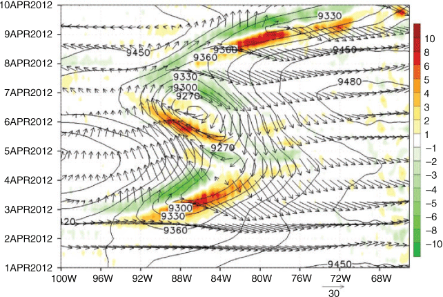
The Hovmoller graph (Fig. 10). shows a marked increase of PV in the high troposphere (300 hPa between 95°W and 73°W and between 27.5°S and 22.5°S from 2 to 5 April). Below the minimum value of the PV, a low pressure core was formed and can be identified by its geopotential height (5670 m) at 500 hPa, accompanied by intense winds that exceeded 30 m s−1, especially west of the cyclonic system. Likewise, the cyclonic core is explained by the deepening of the extratropical trough associated with the maximum winds of the Subtropical and North Polar jets (Jet Streaks), cooling from higher to medium levels. These factors contributed to the collapse of the tropopause by the cold thermal anomaly in the middle troposphere.
|
6 Quasi-geostrophic equations analysis
When analysing the advection of absolute vorticity in higher levels (figure not shown) the COL appeared as a more intense negative absolute vorticity advection to the west of the system, which persisted throughout the COLs development until its maturity stage. This allowed the system to maintain a cyclonic turn and even deepen in time. Days after 5 April, positive absolute vorticity advection predominated over the negative absolute vorticity due to a ridge between 110°W and 90°W that advected positive vorticity from its centre (axis of the ridge) and caused the decay of the COL, as the system did not have cyclonic contribution.
Considering the thickness advection in the 400–700 hPa layer (figure not shown), on 2 April, negative thickness advection to the west of the COL was observed as time continued; then, on 5 April, the core of the COL showed a minimum at the geopotential height of 5560 m, and the negative thickness advection west of its core continued to spread throughout it.
At the same time, the advection of cold air at lower levels (figure not shown) followed a similar pattern, with a maximum cold advection to the west of the system and in its core. Some authors suggest that cold advection at lower levels lengthens the life of the system at higher levels (e.g. Campetella and Possia 2007).
The COL was triggered by the amplification of a ridge west of its location, as well as the presence of a shortwave trough embedded in the ridge, which encouraged the deepening of the COL by intensifying the jet stream.
The evolution of the COL is observed through all the component A of the geopotential tendency equation every 24 h (Fig. 11). Between 1 and 5 April, the COL travelled towards the northeast until it reached its maximum depth, which was favoured by the maximum cold advection at lower levels. After reaching its maximum geopotential fall, the COL changed direction towards the southwest, associated with lower levels of cold advection and vorticity advection at higher levels. On 8 April, the COL experienced significant increase in its geopotential tendency, which favoured it’s deepening and northeast movement; however, it did not maintain a similar evolution as before and dissipated on 9 April.

|
The evolution of the COL can also be seen in a Hovmoller graph of component A of the geopotential tendency equation in a cross section at 25°S (Fig. 12). The behaviour of its irregular movement is appreciated, which depended on the components of the quasi-geostrophic equation in both higher and lower levels. Considering this, term A can be used to predict the COLs movement.
|
7 Analysis of satellite imagery
The water vapour image of the Geostationary Operational Environmental Satellites (GOES)-12 (Fig. 13a) shows the presence of subsidence along 30°S that extends towards the southeast of the eastern Pacific, crossing the Andes at southern Chile. Such behaviour is associated with the presence of vertical shear caused by the jet stream in high troposphere, which evolved with a wave towards the north while a trough deepened and later became a COL at 30°S–90°W. The thermal contrast associated with the incursion of southern flows (darker region) progressed favourably towards the north of its initial location for the days following 2 April. On the other hand, the Amazon basin and the eastern Peruvian Andes showed humidity, helped by the eastern flows that in turn were attracted by the presence of the COL over the eastern Pacific on 5 April (Fig. 13b).

|
The strong injection of cold air from subtropical latitudes was advected to the north and was gradually enveloped in the core of the COL. At the same time, the northern air from warmer and more humid areas enveloped the COL, and consequently, the system was invaded by warmer air that caused its decay. The warmer air incursion blocked the COL and prevented its advance towards the east. A similar behavior was found by Fuenzalida et al. (2005); Garreaud and Fuenzalida (2007) and Godoy et al. (2011).
Along the central and northern coast of Peru, the wind field (Fig. 13c) at lower levels was influenced by the cyclonic circulation of the COL, as shown in Figs 5 and 6. Also, Fig. 8 shows the displacement of humidity along the central coast favoured by the wind field at lower levels. This wind pattern shows the incursion of the wind into the Rímac basin, which forced the confinement of moisture in the basin. In addition to the vorticity advection shown in Fig. 6, and as explained previously, the infrared image (Fig. 13c) evidences unusual convection for the region (see yellow and green coloration), with cloud top temperatures up to –47°C and vertical development that led to the unusual precipitation along the western Andes.
8 Rainfall analysis in Chosica
The rainy season (September–June) in the Andean tropical region is also known as the hydrological year; the maximum intensities and rainfall occur between the months of December and March. During this period, thunderstorms, hail and snowfall are also common, mainly in areas above 3000 masl. Nevertheless, the arid coast and the western foothills of the Andean cordillera show a scarcity of precipitation throughout the year, and in the rainy season it is difficult to reach values higher than 20 mm a year.
However, during the first days of April 2012, with a COL in tropical latitudes near the coast of the South America, heavy precipitation occurred along the western Andes. The greatest impact caused by the rain on 5 April was in the locality of Chosica, with a 37 mm record that day, exceeding its 10 day normal by over 300% (Fig. 1); at the same time there were other areas with similar anomalies of precipitation, mainly in the south coast of Peru (Moquegua and Arequipa); but Chosica was the most affected as the basin is not well suited for such amounts of rainfall, which caused flash floods and landslides.
For the rainfall analysis, we used data from two SENAMHI weather stations located in Chosica. The first is a conventional weather station that was active between November 1947 and March 1955, re-launched in 1990 and have been active since; the second is an automatic hydrometeorological station, which has been active since March 1989 but with incomplete data for the years 1997, 1998, 2009 and 2012 (1997 was not considered since the station was inactive most of the year). The average annual precipitation was 23 mm (29 years; discontinuous). The highest rainfall record corresponds was 64.6 mm in 2012 (Fig. 14), which was more than half of the rainfall (57%) registered during the event of 5 April. The lowest annual rainfall was 1.1 mm in 2010.

|
8.1 Rainfall on April 2012
The average rainfall for the month of April was 2.1 mm; however, when excluding data from 2012, this drops to 0.9 mm. Considering this and that the median precipitation of the series is 0.1 mm, the event that was recorded on 5 April 2012 constitutes an exceptional anomaly. If we review the rainfall record for the month of April, the only other time the monthly rainfall exceeded 5 mm was in 2007, which highlights April 2012 with its 37.4 mm.
8.2 Daily rainfall
The analysis of daily maximum precipitation for the station of Chosica shows again the exceptionality of the rainfall registered on the day of the event, with 37.4 mm recorded in a period of 6 h. However, another extraordinary event was detected on 5 February 2002 with 30.7 mm, which also caused serious problems in the district. If we do not consider the two exceptional events recorded on 5 February 2002 and 5 April 2012, a homogeneous distribution of the maximum daily rainfall (gray) is observed, with a maximum in January and a progressive decrease towards the months of winter (dry season) that increases again at the end of the year with the start of the rainy season. Thus, these two exceptional events are very important anomalies in the daily maximum rainfall series.
The reanalysis data of 5 February 2002 (figure not shown) does not show the presence of a COL in tropical latitudes that directly affected the western Andes. At this time, there was high undulation at higher levels, and the presence of the BH over Peru, with its core located on the Gulf of Arica. Therefore, we cannot directly and exclusively associate the presence of extreme rainfall in the locality of Chosica to the existence of a COL in tropical latitudes.
On the other hand, on 5 April 2012, the automatic hydrometeorological station began to register precipitation at 21:00 UTC with 0.1 mm. After that, the rain increased in intensity measuring 13.9 mm at 22:00 UTC and 11.4 mm at 23:00 UTC then decreasing to 1.5 mm at 00:00 UTC and then less than 1 mm by 03:00 UTC when the rainfall stopped. Therefore, the highest rainfall intensity occurred between 22:00 and 23:00 UTC.
Another interesting feature that emerged from the data is the change of wind direction going from southwest to northeast at the beginning of the event; Chosica is located at 850 masl in the valley of the Rimac River, a valley that has a SW–NE orientation, flanked by mountains that reach 2000–2300 masl. Generally, valley winds with moderate intensities prevail in the afternoon because of the huge gradient between the lower part of the valley (0 masl) and the higher areas (>5000 masl); but during the event of 5 April 2012, these valley winds were canceled, with northeast winds coming from the upper part of the valley, winds that usually appear during the night hours (katabatic winds).
9 Conclusions
A circulation pattern of a COL, which is infrequent in tropical latitudes in southwestern Peru (Fig. 2), occurred on 5 April 2012 and favoured convective activity on the western Peruvian Andes, causing intense rainfall in arid areas.
The life cycle of the COL analysed in this study, began on 2 April 2012 with the amplification to the south (higher latitudes) of a ridge in the southeast Pacific, which encouraged the deepening and displacement of the ridge towards the north of a trough located off the central coast of Chile. During the development stage, the thickness advection in medium and lower layers, as well as the advection of cyclonic vorticity in higher levels, favoured intensification and subsequent segregation of the trough. The COL reached tropical latitudes (below 23°S) on 5 April 2012, with its maximum intensity and northernmost position at 00:00 UTC, which is shown in the water vapour satellite image (Fig. 13). Also, a marked increase of PV in the high troposphere denotes the lowering of the tropopause, which reached 500 hPa in the core of the COL at 00:00 UTC on 5 April. The behaviour of the irregular movement of the COL can be predicted with the term A of the tendency geopotential equation.
The circulation pattern of the COL favoured the formation of convective nuclei on the western Andes (Peru) with moderate rainfall intensity in arid areas close to the coast. In particular, one convective event was analysed that formed in high areas of the Chancay River basin, which, in its movement to the southeast, affected the locality of Chosica, causing the death of 2 people and serious material damage between 22:00 UTC 5 April and 00:00 UTC the following day. The analysis of the precipitation in this area showed the exceptionality of the event, which reached 37 mm that day and had a maximum intensity of 14 mm h−1; this turned out to be the highest recorded daily rainfall of the entire historical series.
Alongside the COL effect on the heavy precipitation event between 2 and 5 April, this persistent coastal trough along the west coast of South America, with associated coastal lows, could be an additional factor in the destabilisation of the atmosphere on the western Andes. This would need further research in futures studies.
Conflicts of interest
The authors declare that they have no conflicts of interest.
Acknowledgements
This research was supported by the National Hydrometeorological Service of Peru (SENAMHI).
References
Bell, G. D., and Bosart, L. A. (1993). A case study diagnoses of the formation of an upper-level cutoff cyclonic circulation over eastern United States. Mon. Wea. Rev. 121, 1635–1655.| A case study diagnoses of the formation of an upper-level cutoff cyclonic circulation over eastern United States.Crossref | GoogleScholarGoogle Scholar |
Campetella, C. M., and Possia, N. E. (2007). Upper-level cut-off lows in southern South America. Meteorol. Atmos. Phys. 96, 181–191.
| Upper-level cut-off lows in southern South America.Crossref | GoogleScholarGoogle Scholar |
Dee, D. P., Uppala, S. M., Simmons, A. J., Berrisford, P., Poli, P., Kobayashi, S., Andrae, U., Balmaseda, M. A., Balsamo, G., Bauer, P., Bechtold, P., Beljaars, A. C. M., Van de Berg, L., Bidlot, J., Bormann, N., Delsol, C., Dragani, R., Fuentes, M., Geer, A. J., Heimberger, L., Healy, S. B., Hersbach, H., Hólm, E. V., Isaksen, L., Hallberg, P., Kohler, M., Matricardi, M., McNally, A. P., Monge-Sanz, B. M., Morcrette, J.-J., Park, B.-K., Peubey, C., De Rosnay, P., Tavolato, C., Thépaut, J.-N., and Vitart, F. (2011). The ERA-Interim reanalysis: configuration and performance of the data assimilation system. Quart. J. Roy. Meteorol. Soc. 137, 553–597.
| The ERA-Interim reanalysis: configuration and performance of the data assimilation system.Crossref | GoogleScholarGoogle Scholar |
Fuenzalida, H. A., Sánchez, R., and Garreaud, R. D. (2005). A climatology of cutoff lows in the Southern Hemisphere. J. Geophys. Res. 110, D18101.
| A climatology of cutoff lows in the Southern Hemisphere.Crossref | GoogleScholarGoogle Scholar |
Garreaud, R. D., and Fuenzalida, H. A. (2007). The influence of the Andes on Cutoff Lows: a modeling study. Mon. Wea. Rev. 135, 1596–1613.
| The influence of the Andes on Cutoff Lows: a modeling study.Crossref | GoogleScholarGoogle Scholar |
Godoy, A. A., Campetella, C., and Possia, N. (2011). Un caso de baja segregada en el Sur de Sudamérica: Descripción del ciclo de vida y su relación con la precipitación. Rev. Bras. Meteorol. 26, 491–502.
| Un caso de baja segregada en el Sur de Sudamérica: Descripción del ciclo de vida y su relación con la precipitación.Crossref | GoogleScholarGoogle Scholar |
Holton, J. R. 2004. ‘An Introduction to Dynamic Meteorology’. Fourth Edition. (Elsevier Academic Press: Washington, USA).
Hoskins, B. J., McIntyre, M. E., and Robertson, A. W. (1985). On the use and significance of isentropic potential vorticity maps. Quart. J. Roy. Meteorol. Soc. 111, 877–946.
| On the use and significance of isentropic potential vorticity maps.Crossref | GoogleScholarGoogle Scholar |
Hoskins, B. J. (1991). Towards a PV-Theta view of the general circulation. Tellus B 43, 27–35.
| Towards a PV-Theta view of the general circulation.Crossref | GoogleScholarGoogle Scholar |
INDECI 2004. Compendio Estadístico del SINADECI 2004. 34 pp. Available at https://bit.ly/3irKRnl [In Spanish]
INDECI 2012. Informe de Emergencia N° 321 - 13/04/2012/COEN-INDECI/17:00 horas (Informe N° 09). 20 pp. Available at https://rb.gy/zbypvp [In Spanish]
Palmén, E. (1949). Origin and structure of high-level cyclones south of the maximum westerlies. Tellus 1, 22–31.
| Origin and structure of high-level cyclones south of the maximum westerlies.Crossref | GoogleScholarGoogle Scholar |
Palmer, C. E. (1951). On high level cyclones originating in the tropics. Eos Trans. AGU 32, 683–696.
| On high level cyclones originating in the tropics.Crossref | GoogleScholarGoogle Scholar |
Pinheiro, H. R., 2010. Validação do método Track para identificação objetiva dos vórtices ciclônicos de altos níveis em regiões subtropicais. MSc Dissertation, INPE, S. J. Campos, SP, Brazil, 132 pp.
Quispe, N. and Avalos, G., 2006. Intense snowstorm in the southern mountains of Peru associated to the incursion a cut-off low pressure system at upper level. Proceedings 8th ISHCMO, 4, 2006, Foz do Iguaçu, Anais. Brasil: Editora, 2006. 1 CD-ROM.
Rondanelli, R., Gallardo, L., and Garreaud, R. D. (2002). Rapid changes in ozone mixing ratios at Cerro Tololo (30°10′S, 70°48′W, 2200 m) in connection with cutoff lows and deep troughs. J. Geophys. Res. 107, 4677.
| Rapid changes in ozone mixing ratios at Cerro Tololo (30°10′S, 70°48′W, 2200 m) in connection with cutoff lows and deep troughs.Crossref | GoogleScholarGoogle Scholar |
Stein, A. F., Draxler, R. R., Rolph, G. D., Stunder, B. J. B., Cohen, M. D., and Ngan, F. (2015). NOAA’s HYSPLIT Atmospheric and Dispersion Modeling System. Bull. Amer. Meteor. Soc. 96, 2059–2077.
| NOAA’s HYSPLIT Atmospheric and Dispersion Modeling System.Crossref | GoogleScholarGoogle Scholar |
Thorncroft, C. D., Hoskins, B. J., and McIntyre, M. E. (1993). Two Paradigms of baroclinic-wave life-cycle behavior. Quart. J. Roy. Meteorol. Soc. 119, 17–55.
| Two Paradigms of baroclinic-wave life-cycle behavior. Quart.Crossref | GoogleScholarGoogle Scholar |
Van Delden, A., and Neggers, R. (2003). A case study of tropopause cyclogenesis. Met. Apps. 10, 187–199.
| A case study of tropopause cyclogenesis.Crossref | GoogleScholarGoogle Scholar |
World Meteorological Organization (WMO), (1986) Scientific assessment of ozone depletion, 1986. Rep. 16, Global Ozone Res. and Monit. Proj., Geneva, 264p.
Wood, R. (2012). Stratocumulus Clouds. Mon. Wea. Rev. 140, 2373–2423.
| Stratocumulus Clouds.Crossref | GoogleScholarGoogle Scholar |