Analysis of a southerly buster event and associated solitary waves

Additional keywords: coastally trapped disturbance, density currents.

Southerly busters (SBs) occur during the spring and summer months in south-east Australia, to the east of the Great Dividing Range (GDR) (Fig. 1), along the coast of New South Wales (NSW) from ∼38 to 30°S. They are strong, sudden and squally southerly wind surges (e.g. Colquhoun et al. 1985; McInnes 1993; Reid and Leslie 1999). The depth of the surge is generally less than 1 km. The SB passage is notable for the typical wind shift from north-westerly to southerly and for the sudden temperature decreases of up to 20°C within minutes (Gentilli 1969). More precisely, SBs are defined as ‘squally wind change that produce strong southerly winds near the coast with gusts to at least 15 m/s soon after their passages and which are not associated with a major depression over the Tasman Sea at New South Wales latitudes’ (Colquhoun et al. 1985). Strong SBs (SSBs) are defined as those with wind gusts of at least 21 m/s, which is the issuance criterion for airport warnings of expected damaging winds. SBs are particularly intense examples of thermally and orographically influenced cold fronts. They occur because inversions ahead of the cold front prevent the vertical escape of energy, and Coriolis effects trap the energy against the GDR (Colquhoun et al. 1985; Gill 1977).

Fig. 1.  Topography of New South Wales Pacific Ocean coast from Nowra to Sydney, with the Great Dividing Range to the west of Nowra, Bellambi and Sydney in metres. The map includes the regional district boundaries and the elevation bands are in metres. The heights just west of Nowra Airport (YNSW) typically are ∼500 m and west of Sydney Airport (YSSY) are ∼1000 m.

SBs also have been investigated under other names. These designations include ducted coastal ridging, which is an atmospheric surge over coastal south-east Australia, moving at a speed of ∼20 m/s at the leading edge of the ridge (Holland and Leslie 1986). The coastal ridging is initiated by a forced Kelvin-type edge wave which forms on the south-west end of the GDR, in coastal western Victoria, and is ducted, anticlockwise, around the coast. The ridge then is stabilized by inertial modification and decays on a synoptic timescale of a few days (Holland and Leslie 1986). Another widely used term is coastally trapped disturbances (CTDs), following the study by Gill (1977) of the coastal lows observed moving anticlockwise around southern Africa. Coastal lows are similar in structure to coastally trapped waves in the ocean. As in the case of SBs, inversion conditions typical of the area prevent the escape of energy upwards, and Coriolis effects trap energy against the high escarpment that borders the southern African coast. Hence, CTDs are produced because low-level flow in the synoptic-scale systems cannot cross the escarpment (Gill 1977). The term CTD also has been used frequently for south-eastern Australia SBs (e.g. Reason 1994; Reason and Steyn 1990, 1992; Reason et al. 1999). Notably, the consensus is that the SB is a gravity current, also known as a density current, trapped against the coast by the GDR (e.g. Baines 1980; Mass and Albright 1987; Egger and Hoinka 1992; McInnes 1993; Reid and Leslie 1999). As such, it is initiated by a synoptic scale system and is generated by the density difference between the cooler southerly flow and the in situ warmer environment ahead of the surge.

Due to the rapid wind and temperature changes, SBs frequently are accompanied by low cloud, fog, thunderstorms and gusty winds. Consequently, SBs are a potential threat for human health, lives and property. In the case of aviation, there are numerous aircraft hazards that often result from the low-level wind shear associated with the SBs, especially during take-off or landing. The main consequences of wind shear include turbulence, violent air movement (e.g. abrupt up and down draughts, and swirling, or rotating, air patterns), sudden increases or reductions of airspeed and rapid increases or decreases of groundspeed and/or drift. The strong winds and associated low level turbulence also are hazards for boating, especially as SBs occur along the populous south-east seaboard of Australia. For marine activities such as surfing, rock fishing and boating, each year marine rescue organizations respond to thousands of calls for assistance from NSW coastal waters; many are related to the passage of SBs, which can produce sudden strength to gale force coastal winds and generate dangerously high waves and choppy seas.

In this study, the SB event of 6–7 October 2015 is examined with the high temporal and spatial resolution observational data that was not available in the earlier studies mentioned above. As mentioned above, an SB is viewed as a density current advancing into a strongly stable in situ boundary layer which comprises warm summertime prefrontal continental air advection overlaying a cooler sea. Frequently a roll vortex is generated, which extends ahead of the cold front, in about half of observed SBs (Colquhoun et al. 1985; http://www.eumetrain.org/satmanu/CM4SH/Australia/ShCF/navmenu.php, accessed 29 April 2020). The head of the density current breaks away from the feeder flow supplying it with cold air and the prefrontal boundary layer commonly is between 100 and 200 m deep and, if the prefrontal stable layer is deep and strong, the roll vortex can evolve as a solitary wave, or as a bore wave, that propagates on the stable layer.

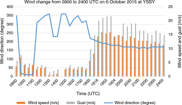
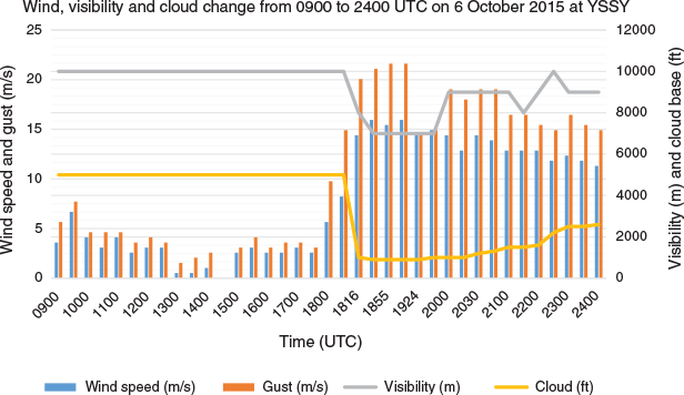
On 6 October 2015, a southerly wind change (SC) propagated along the south-east coast of Australia. At Nowra Airport (YSNW), the winds were moderate (5–10 m/s) west to north-westerly during the day, from 0000 UTC (Coordinated Universal Time) to 0730 UTC, due to the synoptic winds ahead of the trough. The winds became light and variable in the evening (0730–1200 UTC) and then trended to north-west drainage flow around or below 5 m/s before the SC occurred (Fig. 2). At 1559 UTC, the SC arrived at YSNW with southerly winds of 8 m/s, gusting to 11 m/s, at the automatic weather station (AWS) site which is 112 km south of Sydney Airport (YSSY). At 1630 UTC, the SC wind gusts touched 15 m/s, thereby officially becoming an SB, then decreased over the following 90 min. The SC arrived at YSSY at 1800 UTC and became an SB just 2 min later. The wind gusts reached 21 m/s which met the criterion for an airport warning at YSSY (Fig. 3 and Table 1). At YSSY, ahead of the SC, there was light-to-moderate north-west drainage flow ∼3–4 m/s; at 1800 UTC, the observations showed nil significant cloud and the wind direction changed from north-west to south to south-west, the wind speeds picked up at 1802 UTC with gusts to 15 m/s, hence reaching SB levels. Approximately 16 min later, at 1816 UTC, some low clouds developed at ∼300 m; at the same time, the visibility dropped to ∼2300 m, or 7000 ft (Fig. 4). Another key signature was a sudden pressure rise of up to 6 hPa after the SC, within 3 h, at both YSNW and YSSY. This pressure rise had become noticeably steeper, starting at Mt Gambier and reached a maximum amplitude and steepness from Nowra (6.2 hPa) to YSSY (6.4 hPa). The rapid pressure rises associated with the coastal ridging that occur behind the SC are a signature feature of the main CTD (Holland and Leslie 1986).

Fig. 2.  Observations of wind change from 0000 to 2330 UTC on 6 October 2015 at Nowra Airport (YSNW). Time in UTC for horizontal axis, wind directions in degrees for primary vertical axis (left), wind speed gusts in m/s for secondary vertical axis (right). Wind speeds (orange clustered columns, m/s), wind gusts (grey clustered columns, m/s) and wind directions (blue lines, degrees).

Fig. 3.  As in Fig. 2, except at Sydney Airport (YSSY) from 0900 to 2400 UTC on 6 October 2015.

Table 1.  Details of the wind changes at Nowra Airport (YSNW) and Sydney Airport (YSSY)
The southerly change (SC) and southerly buster (SB) time and maximum SB occurring time and winds details, including wind direction (degrees), speed and gust (m/s): e.g. 19008G11 means the wind direction is 190°, the mean wind speed is 08 m/s and the gust wind speed is 11 m/s

Fig. 4.  Observations of wind, visibility and cloud change from 0900 to 2400 UTC on 6 October 2015 at Sydney Airport (YSSY). Time in UTC for horizontal axis, wind speeds and wind gust in m/s for primary vertical axis (left), visibility in metres and cloud base in feet for secondary axis (right). Wind speeds (blue clustered columns in m/s), wind gusts (orange clustered columns in m/s), visibility (grey lines in metres) and cloud base (yellow lines in feet).

The synoptic situation is obtained from archived upper level and mean sea level pressure (MSLP) charts. At 850 hPa on 0000 UTC 5 October 2015, a high-pressure system dominated much of south-east Australia with warm temperatures up to 19°C, whereas a low pressure system with cooler temperatures extended a NW–SE orientated trough from south-west of Australia, crossing the Southern Ocean south of Tasmania. At 1200 UTC October 5, the high moved slowly south-west, whereas the trough moved north-east. By 0000 UTC October 6, the high-pressure centre had moved over the Tasman Sea, and the trough was situated further to the north-east.

A phenomenon well-known to Australian meteorologists is the rapid establishment of a strong coastal ridge, which occurs when a Southern Ocean anticyclone approaches south-eastern Australia. This ridging is initiated by a high-pressure surge which begins off the coast of southern Victoria, then moves rapidly along the NSW coast and often travels along most the entire east coast of Australia, a distance of 2000–3000 km. In contrast, the parent anticyclone moves only several hundred kilometres (Holland and Leslie 1986). The MSLP charts from 0600 UTC 6 October to 1800 UTC 7 October 2015 are shown in Fig. 5. At 0600 UTC October 6, coastal ridging was initiated at the south-western extremity of the GDR, between Mt Gambier and Cape Otway, associated with the northward movement of cold air behind a nearly zonal Southern Ocean front. East of Mt Gambier the cold flow was blocked by the southern slopes of the GDR, thereby driving the ducted disturbance eastwards along the Victorian coast. At 1200 UTC October 6, the coastal ridging had propagated around the south-east corner of Australia and was located on the NSW coast, north of Gabo Island. At 1800 UTC October 6, a strong high-pressure centre (1036 hPa) was situated in the Great Australian Bight, with an inland trough west of the ranges and a frontal zone off eastern Australia, further extending the coastal ridge along the south-east NSW coast. At 0000 UTC October 7, the cold front had continued moving north-east, whereas the high-pressure centre increased to 1039 hPa, strengthening the ridge over south-east NSW. By 1200 and 1800 UTC October 7, the original high-pressure system had separated into two centres, with the parent high remaining over the Southern Ocean and the second centre moving to the south of the Tasman Sea. The coastal ridging had extended along the entire NSW coast and entered southern Queensland.

Fig. 5.  Synoptic weather charts from 0600 UTC October 6 to 1800 UTC October 7 on (a) 0600 UTC 6 October 2015, (b) 1200 UTC 6 October 2015, (c) 1800 UTC 6 October 2015, (d) 0000 UTC 7 October 2015, (e) 1200 UTC 7 October 2015 and (f) 1800 UTC 7 October 2015. Shown are contours of mean sea level pressure (MSLP) in intervals of 4 hPa, local maxima and minima of MSLP, manually analysed cold fronts (solid lines with triangular barbs) and low-pressure troughs (dashed lines) (charts are from http://www.bom.gov.au/australia/charts/, accessed 29 April 2020).

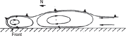
The Himawari-8 satellite image at 2140 UTC on October 6 (Fig. 6) reveals a possible roll cloud accompanying the SB offshore near Williamtown, extending to the south-east over the Tasman Sea. Ahead of the cold front cloud band, what appear to be shallow solitary waves, are moving with the cold front cloud band. Clarke (1961) determined the mesoscale structure of the dry cold fronts using serial pilot balloon flights, radiosonde, and aircraft data. He found closed circulations (roll vortices) in the velocity field behind several fronts; in two cases, double circulations with the roll vortices were inferred (Clarke 1961). A study of 17 SSBs over the period January 1972 to January 1978 was carried out by Colquhoun et al. (1985). Attempts were made to infer the structure of the 17 SBs from anemograph data and temperature profile measurements. The arrival of a clockwise rotating vortex (viewed from the west) was associated with an increase in wind speed and instability and a decrease in temperature; the highest wind speed occurred under the circulation centre of the vortex. Roll vortices were thought to be associated with more than 50% of SBs. The SB frontal structure, in cross section parallel to the coast, is shown for the event of an SB passing YSSY on 11 December 1972 (Fig. 7). Streamlines represent airflow relative to the circulation centres of the roll vortices and straight arrows indicate wind direction. The first circulation cell corresponds with the 28-min period following the first wind change and the second cell with the subsequent 2-h period (Colquhoun et al. 1985). A possibly similar structure appears in the visible satellite imagery on 6 October 2015 (within the green circle of Fig. 6). The roll cloud in the lower atmosphere often exhibits a distinctive flow pattern. Winds near the surface in the horizontal propagating vortices exceed the speed of the propagation and can be a severe hazard to aircraft operating at low altitude (Christie 1983).

Fig. 6.  Himawari-8 satellite visible image at 2140 UTC on 6 October 2015 over the New South Wales coast. Image is shown with the permission of the Australian Bureau of Meteorology. The automatic weather station wind barbs show wind direction and speed in knots (red barbs), and the overlain boundaries of the Australian aviation regions (yellow lines). The green arrow indicates the leading edge of the southerly buster (SB), accompanied by a roll cloud. The yellow arrow points to the low cloud banking up against the escarpment of the range behind the passage of the SB over the eastern Great Dividing Range. The pink arrow locates the parent cold front to the SB. The red arrow shows a possible train of solitary waves. The green circle shows a structure similar to the schematic representation in Fig. 7.

Fig. 7.  Schematic representation deduced from wind temperature data, of the frontal structure in a vertical cross section parallel to the coast. Streamlines are airflow relative to the circulation centres of roll vortices, and straight arrows are wind directions (Colquhoun et al. 1985).

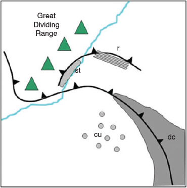
Figure 8 is a schematic of SB cloud signatures detected by the satellite imagery. The acronym, dc, indicates deeper cloud associated with the cold front (seen in visible, infrared and water vapour images); st refers to low (stratus) cloud banking up against the escarpment of the range behind the SB (from visible and, sometimes, infrared images); r denotes roll clouds may be associated with the buster (from visible and, sometimes, infrared images). Finally, cu signifies open cell (speckled) cumulus cloud behind the cold front (from visible and infrared images).

Fig. 8.  Schematic of the cloud signatures of a southerly buster that can be detected using several sources of satellite imagery. From https://sites.google.com/site/cmsforsh/CoE-Australia/shallow-cold-fronts/cloud-structure-in-satellite-images, accessed 29 April 2020.

As mentioned earlier in this section, cloud features associated with the SB also were detected from the Himawari-8 visible imagery at 2140 UTC on 6 October 2015 (Fig. 6). The green arrow indicates the leading edge of the SB accompanied by a roll cloud. The roll cloud is consistent with the schematics of Figs 7 and 8. The yellow arrow points to the low cloud banking up against the escarpment of the range behind the passage of the SB over eastern GDRs. The pink arrow provides the location of the parent cold front to the SB which is consistent with the schematic (Fig. 8). The red arrow (Fig. 6) shows a wave train of solitary waves that propagated ahead of the roll cloud, as expected from Section 3.2, below. Both the solitary waves and the single roll cloud may sometimes be seen at the head of the SB in the visible imagery, although this is not clear in the corresponding infrared images. They can produce wind shear which is sufficiently strong enough to pose a hazard to aircraft operating at low altitudes (typically landing or taking off). Solitary waves in the lower atmosphere take the form of rows of isolated, single-crested gravity, or gravity-inertia waves, which propagate predominantly as clear-air disturbances in a boundary layer inversion waveguide (Christie 1983).

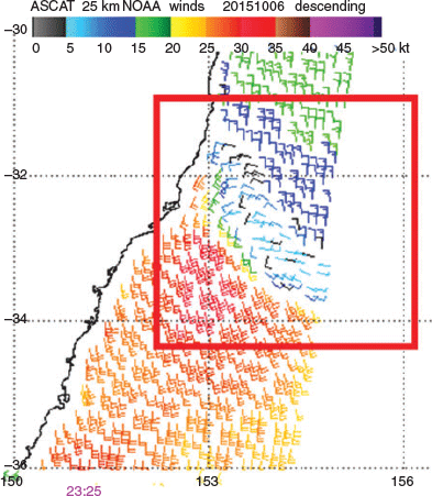
Microwave scatterometer data, such as the winds from the advanced scatterometer (ASCAT) in Fig. 9, also are useful for monitoring SBs, despite this polar orbiting satellite providing data of relatively limited temporal frequency. Fortunately, in this case, descending data was available at 2325 UTC October 6 (Fig. 9). The wind change zone propagated to the north of 32°S and also was detected by the Himawari-8 visible imagery from 2020 to 2320 UTC (Fig. 10). Using both red square boxes in Figs 9 and 10, the SB was well represented for assessing the horizontal structures of the wind change, and for clouds. The transient wind horizontal wind shear in the red box of Fig. 9 clearly is associated with the roll cloud in Fig. 10. The wind speeds behind the change were ∼10–15 m/s, which were responsible for the stratus low clouds near the coast.

Fig. 9.  Advanced scatterometer (ASCAT) winds at 2325 UTC 6 October 2015. Note the detailed near-surface winds, associated with the passage of the SB, in the red square. Image is from the National Oceanic and Atmospheric Administration (NOAA)/National Environmental Satellite, Data, and Information Service (NESDIS) website at https://manati.star.nesdis.noaa.gov/datasets/ASCATData.php, accessed 29 April 2020.

Fig. 10.  The Himawari-8 satellite visible images from 2020 to 2320 UTC 6 October 2015. (a) 2020, (b) 2120, (c) 2220 and (d) 2320 UTC. The green arrow indicates the leading edge of the southerly buster, which is accompanied by a roll cloud. The red arrow shows a train of solitary waves. The solid red line is the distance between the roll cloud and the wave train. The red square in (d) is consistent with the red square area in Fig. 2.

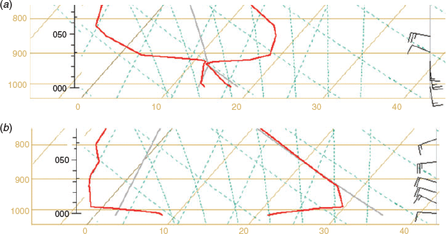
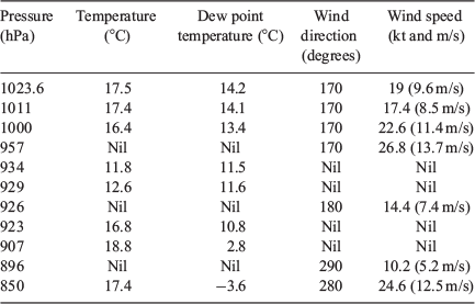
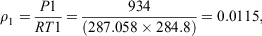
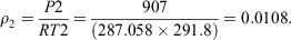
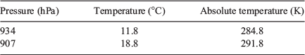
The vertical structure of the atmosphere can be inferred from sounding data from Nowra (YSNW) in Fig. 11a, and Sydney (YSSY) in Fig. 11b. Solitary waves observed in the lower atmosphere typically take the form of rows of isolated, single-crested waves which propagate predominantly as clear-air disturbances in a boundary layer inversion waveguide. The 1700 UTC sounding at YSNW (Fig. 11a), which commenced 1 h after the SB passage, shows a low-level stable layer to 900 hPa overlain by a well-mixed, nearly isentropic layer (neutral layer) extending up to 820 hPa. This configuration is attributed to the advection of the deep continental mixed layer eastwards across the GDR, and then lying over a lower stable marine layer maintained by sea breeze activity along the coast (Holland and Leslie 1986). The low-level southerly winds indicate that the cold air extended to ∼800 m (934 hPa) above mean sea level (MSL). This shallow, stable boundary layer was capped by a strong inversion extending to 1000 m (907 hPa) above MSL. The corresponding temperatures were 11.8°C (at 934 hPa) and 18.8°C (at 907 hPa). The dewpoints were 10.8 and 14.2°C respectively, significantly higher than those above the inversion (Table 2). The dewpoint depressions were no more than 5° below the inversion, then increased abruptly to 20°C at 850 hPa. The winds were moderate to strong southerly below the inversion, and moderate to strong west to north-westerly above the inversion.

Fig. 11.  Radiosonde profile on 6 October 2015 (permission from the Australian Bureau of Meteorology) (a) at 1700 UTC at Nowra Airport (YSNW), (b) at 1900 UTC at Sydney Airport (YSSY). Light brown left vertical axis is pressure (hPa); left black vertical axis is height above sea surface in hundreds of feet. So, e.g. 050 means 5000 ft (∼1600 m) above the sea surface. Right vertical axis is wind profiler information. The red solid lines are the temperature profile (right), and the dew point profile (left). Wind speeds are in m/s; short bar = 2.5 m/s, long bar = 5 m/s.

Table 2.  The Nowra airport (YSNW) radiosonde data on 1700 UTC 6 October 2015, after the SB passage
Nil means no data are available. Note the near-surface stable layer, topped by a neutral layer

At 1900 UTC at Sydney, just ahead of the southerly change, the sounding revealed a strong, shallow inversion from the surface to 50 m above MSL (1000 hPa). Hence, the southerly change is very shallow with an overlying deep inversion. Fronts with a north–west/south–east orientation can experience blocking by the coastal mountain ranges (Fig. 6) of south-east Australia and progressively increase propagation speed on the eastern (coastal) side of the ranges while moving more slowly on the western side of the ranges. The effect is more pronounced for shallow cold fronts than those with the cold-air layer exceeding the height of the ranges (Coulman 1985).

Most of the pressure changes in the postfrontal air of cold fronts are attributable to the density difference between the pre- and postfrontal air masses, and the rate at which the cold air deepens. Propagation speeds also are strongly affected by changes in the density difference (Colquhoun et al. 1985). It is noted that a more rigorous treatment of density currents in stratified shear flows is provided by Liu and Moncrieff (1996) but is beyond that needed in this study. The potential temperature cross sections in figure 7(b) of Colquhoun et al. (1985) are indicative of a density current. The dynamics of coastal ridging is well-described by the hydrostatic approximation, and the shallow-water equations of motion are applicable (Gill 1977; Reason and Steyn 1992). The vertical structure of the coastal atmosphere consists of an inversion, separating a roughly constant density cool marine lower layer from a deep upper layer with weak winds. Note that CTDs do not require the presence of an ocean to exist; it is the presence of stable stratification beneath the crests of the mountain barrier that is essential. There are well-known trapped disturbances occurring over interior plains and confined against large continental mountain ranges elsewhere around the world including, for example, the Rocky Mountains and the Himalayas (Reason 1994).

The density of dry air is calculated from the ideal gas law, expressed as a function of temperature and pressure:

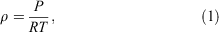
where ρ is the air density (kg/m³), P is the absolute pressure (Pa), T is the absolute temperature (K) and R is the specific gas constant for dry air (287.058 J/(kg·K)).

In the atmosphere, density currents involve the flow (mass transport) of denser air moving into less dense air. For a single layer, the density current flow speed is

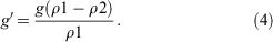
In a two-layer system, which is a good assumption for an SB, with cool air of density ρ1 moving into warm air of lower density ρ2, the density current flow speed is

where the reduced gravity, g′ (m/s²), is

In this case, the density current speed can be estimated, using radio sounding data from the YSNW station.

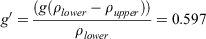
From Eqn 1 and Table 3, for a cooler, denser lower layer overlain by a warmer, less dense upper layer:

Hence, , the density current speed

where

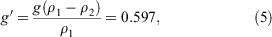
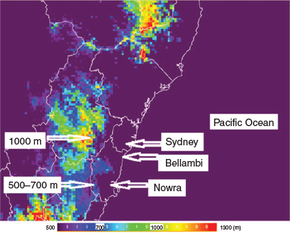
and H, the cold air depth (m) at YSNW, is ∼500 m, from Fig. 6.

Table 3.  Details of the low level structure of the inversion at Nowra airport (YSNW)

So, the density current speed,

The estimated speed in (6) is consistent with the observational data from both the YSNW station observations and also the satellite wind data of Figs 2 and 10, in which the winds in the red square behind the change are ∼15 m/s (∼29 kt). However, it is important to note that the calculation of c_DC is highly dependent on the value of H, so care was taken in selecting the value of H from detailed orographic maps.

It is likely that the parallel cloud lines in the red arrow area solitary waves (Fig. 6), ahead of the SB roll cloud. They are moving slightly faster than the roll cloud (DC). There are at least two possible explanations. One is that trapped density currents can produce solitary waves that are nonlinear Kelvin waves, which move faster than the density current speed (e.g. Ripa 1982), so they propagate through and ahead of the leading edge of the density currents (Reason and Steyn 1990; Reason et al. 1999). The presence of the solitary waves accounts for some of the difficulties in interpreting the precise nature of the leading edge of CTD over coastal south-east Australia. However, there was insufficient observational data before the Himawari-8 satellite, a high spatial and temporal resolution satellite, became available. The Himawari-8 data shows the solitary waves in the visible satellite imagery. A second possibility is that the solitary waves are inertia-gravity waves, also known as Poincaré waves. Like nonlinear Kelvin waves, Poincaré waves also travel faster than the density current. It was decided to proceed with the assumption that the solitary waves are inertia-gravity waves, because nonlinear Kelvin waves eventually break. However, there is no clear sign that the observed solitary waves in this study do break; instead they appear to dissipate after they move well away from the cold front. The formula for the calculation of the phase speed of inertia-gravity (Poincaré) waves is very well-known (e.g. Gill 1982) and is given by

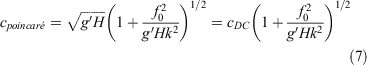
where c_poincaré is the Poincaré wave phase speed (m/s), c_DC is the density current speed (m/s), g′ is the reduced gravity(m/s²) and f₀ is the Coriolis parameter (f = 2Ω sin φ)

where the rotation rate of the Earth, Ω = 7.2921×10⁻⁵ rad/s, can be calculated as 2π/T radians per second, φ is the latitude (Nowra is 34.93°S) and H is the the cold air depth (m), at Nowra (500 m).

The Rossby radius of deformation, , where

Rossby radius of deformation

Wave number k = 2π/wavelength, where wavelength is the Rossby radius of deformation. Thus,

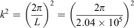
Hence,

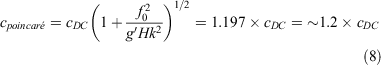
From Eqn 8, the inertia-gravity waves move ∼20% faster than the density current. This difference can explain how, in Figs 6 and 10, the waves move increasingly ahead of the main southerly change, because they are propagating faster than the southerly change.

This study was intended primarily to be a detailed analysis of the SB event of 6–7 October 2015. The parallel cloud lines, revealed by the high-resolution imagery, appear to be solitary waves and are travelling ahead of the SB along the NSW coast. This study has a major advantage over earlier SB studies, due to the access to the much higher temporal and spatial resolution of the Himawari-8 satellite imagery, and other data. The study supported the concept of an SB as a coastal trapped density current, from both the observations and also from the accuracy of the results obtained from the simple density current model. A simple density current model was used to estimate the propagation speed of the SB density current. The estimate of 17 m/s for the density current speed was close to the observed wind speed of ∼15 m/s at Nowra airport. The calculated phase speed of the solitary waves, when assumed to be inertia-gravity (Poincaré) waves, was ∼20% greater than the speed of the density current. Again, this difference was consistent with the satellite imagery, which showed the solitary waves increasingly moving away from the leading edge of the SB. Observations at YSNW and YSSY both exhibit the common characteristics of a classical SB, with an abrupt change in winds, temperatures and pressure. The corresponding weather charts (Fig. 5) illustrate that during the SB event a high-pressure ridge, also referred to as a CTD, generated the SB along the south-eastern Australian coast. Meanwhile, the main high-pressure cell had moved only a few hundred kilometres to the east.

Some interesting questions were raised during the study and will be addressed in future work. Questions raised include the following, and some speculation is made concerning possible answers to these questions. Moreover, answers will be sought from a planned series of very high-resolution numerical modelling simulations of the 6–7 October 2015 SB event.

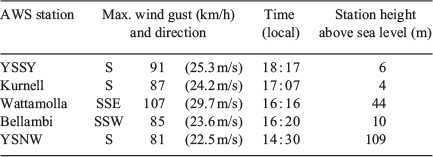
One key question is to determine why was the SB stronger and longer lasting at Sydney airport than at Nowra airport? Possible reasons include the influence of the differences in orography, differential continental heating and differential friction between land and sea. Each of these possible explanations was suggested by Garratt (1986), but supporting observational and modelling evidence was not available at that time. Also, there is related speculation on the effects of coastal irregularities, changes in coastal alignment and land–sea temperature gradients (Holland and Leslie 1986); some of these influences possibly affect the speed and duration of the SB. One factor is the greater distance of Nowra airport from the coast, ∼20 km, whereas the runways of Sydney Airport are adjacent to the water. The Nowra airport location will experience larger frictional effects from the land, which could decouple the motion towards to the north and reduce the propagation speed. Another factor is the possible effects of station elevation: the elevation of Nowra Airport is 109 m, whereas Sydney Airport is only ∼6 m. As stated above, the southerly change is shallow cold air travelling along the coast under the warmer air. From Section 3, the speed of the SB depends on the depth of the cold air according to the formula c = (g′H)^1/2, where g′ is the reduced gravity and H is the depth of the SB. So, as the cold air depth at Nowra Airport is less than at Sydney Airport, the wind speeds in Nowra Airport can be expected to be weaker than at Sydney Airport. An additional possibility is due to the impact of the Illawarra escarpment, west of the Illawarra coastal plain, south of Sydney, with escarpment heights ranging from 300 to 803 m. When the southerly winds travel from Nowra, past Kiama and Wollongong to Sydney, they are blocked from spreading westwards, so cold air mass accumulates along the escarpment and its depth must increase. When they move away from the escarpment, the deeper cold air trapped against the escarpment is released, thereby progressively increasing its propagation speed towards the Sydney Basin, producing stronger southerly winds. A very recent example of the influence on an SB of the Illawarra escarpment and of the station height above sea level, is that of 31 January 2019, is shown in Table 4.

Table 4.  Southerly Buster of 31 January 2019 illustrating differences in maximum gust speed and times at locations Bellambi and Wattamolla adjacent to the Illawarra escarpment and Nowra Airport (YSNW) in the south to Kurnell/Syndey Airport (YSSY) in the Sydney basin to the north
AWS, automatic weather station; S, south, SSE, south-southeast; SSW, south-southwest

Table 4 indicates how the maximum wind gusts increase from 22.5 m/s at Nowra airport to 23.6 m/s Belambi and 29.7 m/s at Wattamolla, then decrease to 24.2 m/s at Kurnell and 25.3 m/s at Sydney airport, after entering wider Sydney basin. Note also the differences in height above sea level of Nowra airport and Wattamolla compared to the other stations. Other interesting questions include why the maximum gust at Sydney airport was ∼50 min after the maximum gust at Kurnell, when the distance between those two locations is only ∼10 km, and was the height difference above sea level between Bellambi and Wattamolla the reason the maximum gust occurred at Wattamolla before Bellambi. As mentioned above, a series of planned high-resolution numerical modelling studies hopefully will provide further insight into the questions raised.

Finally, it is noteworthy that the solitary waves extend east as far as 157°E on the Himawari-8 satellite visible image (Fig. 10), which raises the question of how far east they can travel and has possible safety implications for landing/take-off at Lord Howe Island airport. Again, this question can best be answered with a combination of observations and high-resolution numerical modelling.

References

Baines, P. G. (1980). The dynamics of the southerly buster. Aust. Meteorol. Mag. 28, 175–200.Christie, D. R. (1983). Solitary waves as aviation hazards. Eos. Trans. AGU. 64, 67.