Seasonal climate summary for the southern hemisphere (autumn 2017): the Great Barrier Reef experiences coral bleaching during El Niño–Southern Oscillation neutral conditions

Austral autumn in 2017 followed a year of record high-surface temperature in 2016 that was dominated by a strong El Niño at the beginning of the year and transitioned to weak La Niña–like conditions by the end of 2016 and start of 2017 (National Oceanic and Atmospheric Administration 2017). In Australia for 2016, temperatures were very warm (fourth warmest on record) driven by both El Niño and anthropogenic climate change (Bureau of Meteorology and CSIRO 2017). The Australian national average rainfall in 2016 was ~17% above average.

This summary reviews the climate patterns for Austral autumn 2017, with particular attention given to the Australasian and Pacific regions. The main sources of information for this report are analyses prepared by the Bureau of Meteorology using data sourced from a range of centres and data sets.

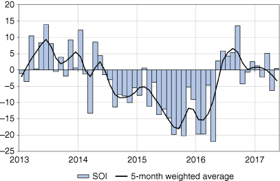
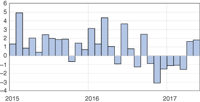
The Troup Southern Oscillation Index (SOI) for the period January 2013 to May 2017 is shown in Fig. 1 (Troup 1965), together with a 5-month weighted moving average to smooth out volatility (Wright 1989). Following positive SOI values for the second half of 2016, the first 5 months of 2017 alternated between positive and negative. The SOI values for March, April and May were +5.1, −6.3, +0.5 respectively, giving a neutral seasonal average of −0.2. The 5-month weighted moving average finished negative at −3.3 at the end of autumn. The monthly mean sea-level pressure (MSLP) anomalies for both Darwin (provided by the Bureau of Meteorology) and Tahiti (provided by the Météo France inter-regional direction for French Polynesia) were near to neutral in the 3-month period (between −0.2 and +0.8 hPa). The 5-month weighted moving average was trending towards negative territory for the autumn period.

Fig. 1.  Southern Oscillation Index (SOI), from January 2013 to May 2017, together with a 5-month binomially weighted moving average. The Troup SOI is 10 times the standardised monthly anomaly of the difference in mean sea-level pressure between Tahiti and Darwin. The calculation is based on a 60-year climatology (1933–92).

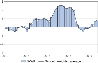
The 5VAR is a composite monthly El Niño–Southern Oscillation (ENSO) Index developed by the Bureau of Meteorology, calculated as the standardised amplitude of the first principal component of monthly Darwin and Tahiti MSLP (data obtained from http://www.bom.gov.au/climate/current/soihtm1.shtml, accessed 29 April 2020) and monthly NINO3, NINO3.4 and NINO4 sea-surface temperatures (SSTs) from the National Centers for Environment Prediction (NCEP), obtained from ftp://ftp.cpc.ncep.noaa.gov/wd52dg/data/indices/sstoi.indices, accessed 29 April 2020 (Kuleshov et al. 2009). Persistent positive or negative 5VAR values in excess of 1 standard deviation are typically associated with El Niño or La Niña events respectively. The monthly 5VAR values for the period January 2013 to May 2017 are shown in Fig. 2, along with the 3-month moving average. The autumn period of March/April/May exhibited mildly positive values of +0.16, +0.75 and +0.72 respectively, which were all below the 1 standard deviation threshold for El Niño events.

Fig. 2.  5VAR composite standardised monthly El Niño–Southern Oscillation (ENSO) index from January 2013 to May 2017, together with a weighted 3-month moving average. The principal component analysis and standardisation of this ENSO index is performed over the period 1950–99.

The multivariate ENSO index (MEI), produced by the Physical Sciences Division of the Earth Systems Research Laboratory (formerly known as the US Climate Diagnostics Centre), is a standardised anomaly derived from a number of atmospheric and oceanic parameters calculated as a 2-month mean (Wolter and Timlin 1993, 1998). As for 5VAR, significant positive anomalies are typically associated with El Niño, whereas large negative anomalies indicate La Niña. The 2017 February/March (−0.08), March/April (+0.74) and April/May (+1.44) values were increasing over the autumn period, similar to the 5VAR, although did not reach significant magnitudes. Contrary to this, rainfall patterns (Section 2.3) and sub-surface Pacific warming (Section 4.2) were more indicative of a weak La Niña signal, and therefore the ENSO indicators pointing towards El Niño had little impact on the Australian climate for autumn 2017.

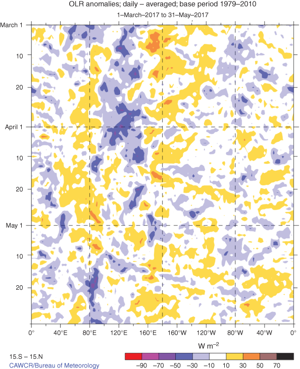
Outgoing long-wave radiation (OLR) is a good proxy for tropical convection and rainfall. Decreased OLR usually indicates increased convection and enhanced associated cloudiness and rainfall, and increased OLR usually indicates decreased convection. During El Niño, OLR is often decreased near the Date Line indicating increased convection (and rainfall) as the Walker Circulation weakens, and the warm pool and associated tropical rainfall is displaced to the east. The reverse is true during La Niña events.

Standardised monthly anomalies of OLR are computed for an equatorial region from 5°S to 5°N and 160°E to 160°W by NOAA’s Climate Prediction Centre (obtained from http://www.cpc.ncep.noaa.gov/data/indices/olr, accessed 29 April 2020). Monthly values for autumn were +1.1, +0.4, +0.1 W m⁻² for March, April and May respectively, indicating that convection was suppressed in that area during autumn. The overall autumn 2017 mean was +0.5, with the countries in the region reporting drought conditions, for example, Kiribati Meteorological Service (2017), and the northern Marshall Islands (UNOCHA ROAP 2017). The spatial patterns of seasonal OLR anomalies across the Asia–Pacific region between 40°S and 40°N for autumn 2017 are shown in Fig. 3. Across Indonesia in locales of Sulawesi, Borneo and West Sumatra, there were reports of widespread floods and landslides during the autumn period (Davies 2017a). Rainfall associated with cyclone Debbie can be seen crossing the Queensland border in Fig. 4. The OLR and rainfall patterns in western Pacific and Indonesia are consistent with a weak La Niña, which is in contrast to what the 5VAR and MEI indicators were suggesting for this period.

Fig. 3.  Outgoing long-wave radiation (OLR) anomalies for autumn 2017 (W m⁻²). Base period is 1979–2000. The mapped region extends from 40°S to 40°N and 70°E to 180°E.

Fig. 4.  Precipitation anomalies for autumn 2017 (mm) for the Pacific region. Base period is 1979–95, from https://iridl.ldeo.columbia.edu/maproom/Global/Precipitation/Seasonal.html, accessed 29 April 2020.

The Indian Ocean Dipole (IOD) describes the pattern of SST anomalies across the equatorial Indian Ocean. A positive phase of the IOD is characterised by cooler than usual water near Indonesia and warmer than usual water in the tropical western Indian Ocean. This pattern is usually associated with decreased convection, and hence less rainfall in the eastern Indian Ocean and across southern Australia during winter and spring. The opposite is true for a negative IOD phase.

IOD events can be represented by the Dipole Mode Index (DMI) (Saji et al. 1999). The DMI is the difference in SST anomalies between the Western Tropical Indian Ocean node centred on the equator off the coast of Somalia (50–70°E and 10°S–10°N) and the Southeastern Tropical Indian Ocean (SETIO) node near Sumatra (90–110°E and 10–0°S). Sustained values of the DMI below −0.4°C indicate a negative IOD event, whereas sustained values above +0.4°C indicate a positive IOD event. An IOD event typically starts from May or June and lasts to around November. A positive IOD event is often associated with below-average rainfall in central and southeastern Australia in spring (Risbey et al. 2009) and is more likely to occur alongside El Niño.

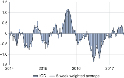
Following a strong negative IOD event that dominated much of 2016, the IOD was mostly weakly positive in autumn 2017. The peak IOD weekly value for this period was +0.38°C (Fig. 5), not quite breaching the threshold value of +0.4°C for a positive IOD event. The SETIO node was dominated by cool anomalies (Fig. 8), as was much of the eastern Indian Ocean. The western and central Indian Ocean saw mostly warm anomalies. This temperature gradient likely contributed to the dry conditions in western and central Australia as it limited the supply of moisture to the atmosphere across the country.

Fig. 5.  Weekly Dipole Mode Index values from January 2014 to May 2017, together with a 5-week binomially weighted moving average. Baseline period is 1961–90. IOD, Indian Ocean Dipole.

The Madden–Julian Oscillation (MJO) can be characterised as a burst of tropical cloud and rainfall which develops over the Indian Ocean and propagates eastwards over to the Pacific Ocean, and sometimes around the entire global equator (Madden and Julian 1971, 1972, 1994). The MJO typically takes 30–60 days to cross from the eastern Indian Ocean to the central Pacific, with six to twelve events per year.

The location of the convective phase of the MJO can be detected by looking for large-scale negative OLR anomalies near the equator and is objectively monitored by the real-time multivariate MJO (RMM) index as described in Wheeler and Hendon (2004). Impacts of the MJO can be felt in many regions of the globe, including outside the tropics (Donald et al. 2004), and its frequency and strength vary from year to year (Wheeler and Hendon 2004). During El Niño years, MJO convection anomalies tend to propagate further eastwards over the warmer waters of the central and eastern Pacific Ocean, but the influence of ENSO on the MJO in other locations is either weaker or not well understood (Hendon et al. 1999).

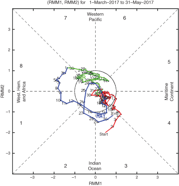
The phase-space diagram of the RMM for autumn 2017 is shown in Fig. 6, and the evolution of tropical convection anomalies along the equator with time is shown in Fig. 7. At the beginning of autumn 2017, the MJO was in an active phase in the Indian Ocean (phase 3) but was soon indiscernible for most of March and April while over the maritime continent and therefore not having an impact on Australian climate. The MJO strengthened back to an active phase at the end of April into the western hemisphere and Africa (phases 8 and 1) until mid of May.

Fig. 6.  Phase-space representation of the Madden–Julian Oscillation (MJO) index for autumn 2017. Daily values are shown with March in red, April in green and May in blue. The eight phases of the MJO and the corresponding (approximate) locations of the near-equatorial enhanced convective are labelled.

Fig. 7.  Time–longitude section of daily-averaged outgoing long-wave radiation (OLR) anomalies, averaged for 15°S to 15°N, for the period March to May 2017. Anomalies are with respect to a base period of 1979–2010.

SST anomalies for autumn 2017 from Optimum Interpolation SST (Reynolds et al. 2002) are shown in Fig. 8. The majority of the tropical Pacific had warm anomalies greater than 0.5°C, with regions in the subtropics and eastern Pacific between 1 and 2°C. The cooler anomalies in extratropical north and south Pacific and warm anomalies elsewhere are consistent with the warm phase of the Pacific Decadal Oscillation that has mostly persisted since 2014. Much of the eastern seaboard of Australia was warmer than average, and conversely, cool anomalies persisted in the southern half off the coast of Western Australia. The most significant warm anomaly in the Australian region was along the east coast of Tasmania extending into the Tasman Sea.

Fig. 8.  Anomalies of global sea-surface temperature (SST) for austral autumn 2017 (°C). Base period is 1981–2010.

The percentile rankings in terms of deciles are shown in Fig. 9. The darkest green indicates the lowest SST on record since 1981, and dark orange is the highest on record. There are significant patches of highest on record within the western warm pool, which typically boasts the highest SSTs in the world. Regions of highest on record for autumn 2017 can be seen in the Pacific subtropics and central Indian Ocean, as well as in the far western Pacific Ocean. Warm waters off the coast of South America have been attributed to causing disastrous flooding rains in both Peru and Chile (Davies 2017b, 2017c). Around Australia, there are emerging regions of highest on record around Tasmania, and conversely, small regions of lowest on record off the southern Western Australia coast.

Fig. 9.  Deciles of global sea-surface temperature (SST) for austral autumn 2017 (°C).

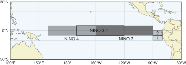
The NINO indices were positive for most of autumn 2017, with NINO4 in March being the only exception having a slightly cool anomaly. The highest anomaly values were in the far eastern Pacific in the NINO1+2 region, although these exhibited a weakening trend over the autumn period, as did NINO3. Both NINO4 and NINO3.4 show warming trends across the autumn period. The NINO3 and NINO3.4 indices are both below the El Niño threshold of +0.8°C, although NINO1+2 values for the autumn period are the highest on record for the index in a year that falls outside of a basin-wide El Niño. For March, only the very strong El Niños of 1983 and 1998 have scored a higher NINO1+2 anomaly, with March 2017 even eclipsing the El Niño 2016 event. See Fig. 10 for locations of the NINO boxes.

Fig. 10.  Locations of NINO boxes in equatorial Pacific Ocean.

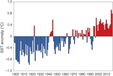
The term coral bleaching refers to the whitening of corals, indicating that the coral has been stressed by a significant change to its preferred environmental conditions which can lead to mortality if adverse conditions persist. In March 2017, the Great Barrier Reef (GBR) experienced its second consecutive mass coral bleaching event following the bleaching event of 2016 (Hughes et al. 2017; Hughes and Kerry 2017). The bleaching driver was elevated SSTs, with the Coral Sea experiencing the second highest autumn SST anomaly since 1900 using the ERSSTv5 data set shown in Fig. 11 (Huang et al. 2017). The only higher anomaly for autumn was in the previous year (2016) which also caused bleaching in the GBR.

Fig. 11.  Autumn sea-surface temperature (SST) anomalies in the Coral Sea for the years 1900–2017 (ERSSTv5). Averaging region for the Coral Sea spans from latitude −4°S to −26°S, and longitude 142°E to 174°E.

Unlike the mass bleaching event in 2016 which was attributed to both climate change and amplified by the 2015/2016 El Niño event (Great Barrier Reef Marine Park Authority 2017), autumn 2017 was classified as ENSO neutral. The event is attributed to two main factors: global warming and local weather patterns. The positive warming trend in the Coral Sea is evident across the SST anomalies in Fig. 11 and supported by IPCC (2013) that states 93% of global warming has occurred in the ocean between 1971 and 2010. In terms of local weather, a relatively low number of summer storms occurred over the Reef until late in the season, leading to increased surface heating and reduced mixing. The SST anomalies at their peak in mid-March (Fig. 12a) were subsequently cooled after the crossing of Cyclone Debbie which made landfall near Airlie Beach (just north of Mackay). The SST anomalies in the northern half of the GBR, which was the primary region of bleaching impact, were largely unaffected by Cyclone Debbie. The final degree heating day (DHD) metric that describes total thermal stress over the 2016/2017 austral summer period is shown in Fig. 12b. Areas of highest stress are shown to be the central third of the GBR.

Fig. 12.  Sea-surface temperature (SST) anomaly 14-day mosaics over the Coral Sea and in the Great Barrier Reef marine park (a) approximate peak of the SST anomaly in March 2017 (b) degree heating days since 1 December, calculated by summing positive 14-day mosaic anomalies. The mosaics are created by aggregating the satellite coverage over the previous 14-day period, giving preference to the most recent observations.

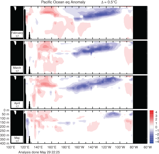
Cross-sectional monthly sub-surface temperature anomalies along the equator, encompassing latitudes 2°S to 2°N, are shown in Fig. 13. The first 2 months of autumn 2017 had a persisting warm anomaly west of the Date Line, and a cold anomaly as low as −3°C stretching eastwards from the Date Line to 100°W that looked similar to what occurs during a La Niña event. However, the month of May saw a significant weakening in this anomaly, resulting in largely neutral conditions throughout most of the equatorial Pacific, with small patches of sub-surface warming in the west and a remaining small cool anomaly close to the surface in the far east.

Fig. 13.  Four-month sequence from March to May 2017 of vertical sea sub-surface temperature anomalies at the equator for the Pacific Ocean. Red shading indicates positive (warm) anomalies and blue shading indicates negative (cool) anomalies. The contour interval is 0.5°C, from http://www.bom.gov.au/oceanography/oceantemp/pastanal.shtml, accessed 29 April 2020.

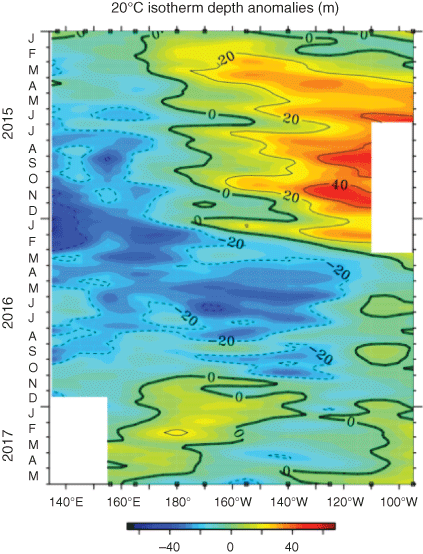
The equatorial thermocline is a region below the surface where the temperature gradient between warm near-surface water and cold deep-ocean waters is greatest. The 20°C isotherm depth is generally located close to this equatorial thermocline. Therefore, measurements of the 20°C isotherm make a good proxy for the thermocline depth. Positive anomalies correspond to a deeper than average thermocline and vice versa, where shifts in the depth of the 20°C isotherm provide an indication of subsequent temperature changes in SSTs; a deeper thermocline results in less cold water available for upwelling, and therefore warming of surface temperatures. The time–longitude (Hovmöller) diagram for the 20°C isotherm depth anomaly along the equator for January 2015 to May 2017, obtained from the TAO Project Office, is shown in Fig. 14.

Fig. 14.  Time–longitude section of the monthly anomalous depth of the 20°C isotherm at the equator (2°S to 2°N) for March to May 2017. From the TAO Project Office: http://www.pmel.noaa.gov/tao/jsdisplay, accessed 29 April 2020.

The 20°C isotherm was elevated in western Pacific at the commencement of autumn 2017. By the end of autumn 2017, the 20°C isotherm was mostly in a neutral position in both the far eastern and western Pacific and slightly suppressed in the central Pacific. By the end of autumn 2017, both sub-surface SST anomies and isotherm location were close to neutral in much of the Pacific, ending the La Niña-like pattern observed over the summer/autumn period.

Sea-level anomalies for autumn 2017 are shown in Fig. 15 and reference a datum of mean sea-surface height from 1993 to 2017. Both the southern Pacific Ocean and Indian Ocean had mostly positive sea-level anomalies. Around Australia, anomalies were also positive, with the highest anomalies experienced in the Gulf of Carpentaria and off the coast of New South Wales (NSW). Flooding associated with the remnants of cyclone Debbie end of March 2017 at Tweed River and Brunswick River (Maddox 2017) were exacerbated by high tides and anomalously high sea levels along the east coast.

Fig. 15.  Sea-level anomalies are a combination of data from TOPEX/Poseidon, Jason-1, Jason-2 and Jason-3 satellites. Inverse barometer effect not removed; seasonal signal not removed; global trend not removed; glacial isostatic adjustment removed. Data obtained from CSIRO Sea Level, Waves and Coastal Extremes: http://www.cmar.csiro.au/sealevel/sl_data_cmar.html, accessed 29 April 2020.

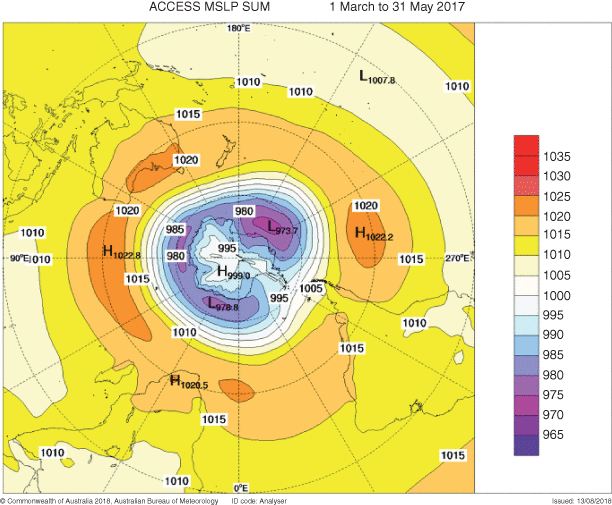
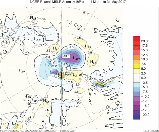
The MSLP pattern for autumn 2017 is shown in Fig. 16, computed using data from the 0000 UTC daily analyses of the Bureau of Meteorology’s Australian Communicate Climate and Earth System Simulator (ACCESS) model (Puri et al. 2013). The MSLP anomalies are shown in Fig. 17, relative to the 1979–2000 climatology obtained from NCEP II Reanalysis data (Kanamitsu et al. 2002).

Fig. 16.  Autumn 2017 mean sea-level pressure (MSLP) (hPa). The contour interval is 5 hPa. The MSLP anomaly field is not shown over areas of elevated topography (grey shading) as the extrapolation to sea level can result in unrealistic structures.

Fig. 17.  Autumn 2017 mean sea-level pressure (MSLP) anomalies (hPa), from a 1979 to 2000 climatology.

The subtropical ridge formed a band of high pressure that was situated below 30°S, extending across the Indian Ocean with a maximum pressure of 1022.8 hPa. Anomalies show that the high-pressure bands were close to climatology for autumn 2017 in the Indian Ocean and across southern Australia. The band of anomalously higher pressure in the Southern Ocean and lower pressure over Antarctica is indicative of a weak positive Southern Annular Mode (SAM) (see Section 5.3). Other high-pressure centres associated with the subtropical ridge were located over South Africa (1020.5 hPa) and off the west coast of Chile (1022.2 hPa). The largest significant low pressure was located at the circumpolar trough off Antarctica between 180 and 270°E, with anomalous pressures of −12.5 hPa. Across the Australian continent, anomalies were generally weak and close to neutral.

The 500-hPa geopotential height, an indicator of the steering of surface synoptic systems across the southern hemisphere, is shown for autumn 2017 in Fig. 18, with associated anomalies shown in Fig. 19. The anomaly patterns show average geopotential height across mainland Australia, with positive anomalies across Tasmania extending to a high of +69 gpm approximately over the Macquarie Island. These positive heights across south of Australia (along with positive MSLP anomalies) reduced the strength of prevailing westerly winds across southern Australia, contributing to a drier southwest Western Australia and Tasmania during autumn. The most significant anomalies in the southern hemisphere are the low of −121 gpm that coincides with the location of the lowest MSLP anomaly in Fig. 17, and a high of +103 gpm over the Antarctic Peninsula.

Fig. 18.  Autumn 2017: 500-hPa mean geopotential height (gpm).

Fig. 19.  Autumn 2017: 500-hPa mean geopotential height anomalies (gpm), from a 1979 to 2000 climatology.

The SAM is a mode of variability that is characterised by the north-south oscillation of westerly winds that encircles Antarctica. An index of SAM is the zonal pressure difference between the latitudes 40 and 65°S (Marshall 2003). During a positive SAM phase, westerly winds contract closer to Antarctica, and a negative phase moves westerly winds towards the equator. Figure 20 shows the SAM index as described in Marshall (2003) from 2015 to the end of autumn 2017 (data obtained from https://legacy.bas.ac.uk/met/gjma/sam.html, accessed 29 April 2020). SAM was mostly positive from 2015 to mid-2016 and was negative for six consecutive months from October 2016 to March 2017. During April and May 2017, SAM returned to the positive phase, which has been shown to reduce rainfall in the far southwest corner of Western Australia in autumn (Hendon et al. 2007).

Fig. 20.  Autumn 2017: 500-hPa mean geopotential height anomalies (gpm), from a 1979 to 2000 climatology.

Low-level (850 hPa) and upper level (200 hPa) wind anomalies are shown in Figs 21 and 22 respectively. Isotach contours are at 5 m s⁻¹ intervals. In the southern central Pacific, there was an anomalous feature that exists in both low (high of 6.6 m s⁻¹) and upper level winds (high of 12.8 m s⁻¹) that is associated with the very strong low-pressure system off the coast of Antarctica (shown in MSLP anomaly Fig. 17). In Australia, the anomalies shown in the low-level are enhanced easterlies across the north and weakened westerlies from the Tasman Sea to the Southern Ocean going over Tasmania. In the upper level, mainland Australia was dominated by an anti-cyclonic system that enhanced the subtropical jet in the southern half and weakened it in the northern half.

Fig. 21.  Autumn 2017: 850-hPa vector wind anomalies (m s⁻¹).

Fig. 22.  Autumn 2017: 200-hPa vector wind anomalies (m s⁻¹).

A rainfall summary for Australia nationwide and each state and territory is listed in Table 1. Rainfall was slightly below average in autumn 2017 over Australia but varied regionally across the country significantly (Fig. 23). Victoria, NSW and Western Australia were slightly above the mean, Queensland was slightly below the mean, and the remainder of the states and territories were well below the mean by an order of 20–30%. Central Australia experienced very much below-average rainfall, primarily in the southern Northern Territory, as did in smaller regions in the far west of Queensland.

Table 1.  Summary of the seasonal rainfall ranks and extremes on a national and state basis for autumn 2017
The ranking in the second last column goes from 1 (lowest) to 118 (highest) and is calculated over the years 1900–2017 inclusive. Qld, Queensland

Fig. 23.  Autumn 2017 rainfall totals (mm) for Australia.

The coastline of Queensland had above-average rainfall from approximately Townsville all the way south along the Queensland and NSW coast to the Victorian border. Western Victoria was mostly above average. Southern Western Australia had very much below-average rainfall in the west; however, the remainder of the state was either average or above average. Severe tropical cyclone Debbie brought heavy rainfall and floods to parts of eastern Queensland and northeastern NSW at the end of March. The two highest daily totals for Queensland and NSW shown in Table 1 (Mount Jukes and Chillingham respectively) for autumn 2017 were associated with cyclone Debbie. Heavy rain in Queensland on 18 and 19 May also contributed to high seasonal totals between the Gulf Country and the tropical and central coasts, with some locations setting monthly rainfall records for May in part due to this event.

Rainfall deciles indicate where rainfall amounts rank in terms of the 1900 to 2017 record, which are allotted into 10 percentile bins (Fig. 24). Above-average rainfall was also observed in western Victoria and adjacent parts of NSW border country and southeastern South Australia; an area of central South Australia; the coastal Top End in the Northern Territory; and areas of Western Australia’s between the southern Kimberley and southern interior, and along a broad strip extending from the eastern Pilbara coast to the western Eucla coast.

Fig. 24.  Autumn 2017 rainfall deciles for Australia: decile ranges based on grid-point values over all autumns from 1900 to 2017.

Rainfall for the season was below average for much of western and southwestern Queensland, extending across the southern half of the Northern Territory; on each of the Yorke, Eyre and Fleurieu peninsula in South Australia; across the west of Western Australia from the far western Pilbara to the south coast around Esperance. In Western Australia the South West Land Division recorded its 11th-driest autumn on record, and driest autumn since 2012, and was the driest autumn for at least two decades at many locations. In Tasmania, western and southern regions were below average.

Rainfall deficiencies are used to indicate areas of drought and are assessed by determining regions in the lowest 10% of records (serious deficiency), lowest 5% (severe deficiency) and lowest on record. Deficiencies for autumn 2017 are shown in Fig. 25. The most prominent region of rainfall deficiency was along the west coast of Western Australia, spanning from Gascoyne, through the Mid-West and into the Wheatbelt. Small regions of lowest on record were experienced near the coast from Carnarvon to Shark Bay. The Northern Territory also had a region of serious-to-severe deficiency south of Tennant Creek reaching across the borders into Queensland and South Australia. Serious rainfall deficiencies also emerged in pockets of the southern South West Land Division in Western Australia and on the Eyre Peninsula in South Australia. In Tasmania, rainfall deficiencies covered the western highlands region.

Fig. 25.  Rainfall deficiencies for autumn 2017.

A subset of the full temperature network was used to calculate the spatial averages and rankings for Australia, and all states and territories shown in Table 2 (maximum temperature) and Table 3 (minimum temperature). This data set is known as ACORN-SAT (see http://www.bom.gov.au/climate/change/acorn-sat/ for details, accessed 29 April 2020) and extends from 1910 to present. The mean maximum temperature for autumn 2017 was +1.21°C above average for Australia, ranking seventh warmest out of 108 autumn periods on record. All states except NSW and Western Australia ranked in the top 10 autumns for maximum temperature. Regions in western Queensland and into the Northern Territory were highest on record. National mean minimum temperatures were +0.42°C above average, although only Queensland, Victoria and Tasmania were within the top 10 autumns for minimum temperature.

Table 2.  Summary of the seasonal maximum temperature ranks and extremes on a national and state basis for autumn 2017
The ranking in the last column goes from 1 (lowest) to 108 (highest) and is calculated over the years 1910–2017 inclusive. As the anomaly averages in the tables are only retained to two decimal places, tied rankings are possible. AWS, automatic weather station; NSW, New South Wales; Qld, Queensland; Vic., Victoria; WA, Western Australia

Table 3.  Summary of the seasonal minimum temperature ranks and extremes on a national and state basis for autumn 2017
The ranking in the last column goes from 1 (lowest) to 108 (highest) and is calculated over the years 1910–2017 inclusive. As the anomaly averages in the tables are only retained to two decimal places, tied rankings are possible. AWS, automatic weather station; NSW, New South Wales; SA, South Australia; WA, Western Australia

Maximum temperatures for autumn (Figs 26 and 27) were above to very much above average for most of the Northern Territory, along the eastern border of Western Australia south of the Kimberley, across all of South Australia, most of Queensland, inland NSW, all of Victoria and very much above average for all of Tasmania, and an area of Western Australia between the western Pilbara and Central Wheatbelt. There was a region of warmest on record for autumn in western Queensland, reaching across the border into the Northern Territory.

Fig. 26.  Autumn 2017 maximum temperature anomalies (°C) from analysis of ACORN-SAT data.

Fig. 27.  Autumn 2017 maximum temperature deciles from analysis of ACORN-SAT data: decile ranges based on grid-point values for all autumns from 1910 to 2017.

Mean minimum temperatures (Figs 28 and 29) were also above to very much above average for most of eastern Australia, the east of South Australia, and the northern half and far southeast of the Northern Territory. Minimum temperatures were mostly near average for Western Australia during autumn, although they were cooler than average for an area spanning the southwestern Northern Territory and the adjacent eastern interior and southeastern Kimberley in Western Australia. There was a small region of very much below-average minimum temperatures on the Western Australia coast west of the South Australia border, and additional pockets of below-average minimum temperatures on northeast of the Wheatbelt and near Karratha.

Fig. 28.  Autumn 2017 minimum temperature anomalies (°C) from analysis of ACORN-SAT data.

Fig. 29.  Autumn 2017 minimum temperature deciles from analysis of ACORN-SAT data: decile ranges based on grid-point values for all autumns from 1910 to 2017.

Temperatures in the southern hemisphere were the warmest on record for land and ocean in autumn 2017 according to the National Aeronautics and Space Administration data set (Hansen et al. 2010), second warmest on record for land and ocean in the National Oceanic and Atmospheric Administration (NOAA) data set (Smith and Reynolds 2005), and third warmest in the United Kingdom Meteorological Office Hadley Centre/Climatic Research Unit, University of East Anglia (HadCRU) data set (Morice et al. 2012). The differences in ranks between the three data sets reflect the different methods they use for assessing temperatures over data-sparse land measurements and are typically greater in the southern hemisphere than the northern due to the lower data density.

Land temperatures in autumn 2017 were mostly warmer than average in the southern hemisphere, with the only significant exception being the southwest coast of Western Australia (Fig. 30). Both southern Africa and eastern Australia had significant expanses of up to +1°C warmer than the 1981–2010 average. South America was mostly up to +0.5°C warmer than average. New Zealand’s North Island experienced temperatures up to +1.2°C above the 1981–2010 average, with even higher temperatures in the Bay of Plenty and Auckland (NIWA 2017).

Fig. 30.  Mean temperature anomalies (°C) from a 1981–2010 base period for March to May 2017 (source: National Centers for Environmental Information).

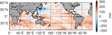
Seasonal precipitation percentages with reference to normal from 1951 to 2000 are shown for autumn 2017 in Fig. 31. Above-average seasonal precipitation was observed across the west coast of, and southern, South America, with severe flooding reported in Argentina, Peru and Chile (Davies 2017b, 2017c; World Meteorological Organization 2018). Flooding along the west coast of South America is typical in the late phase of El Niño, although autumn 2017 was defined as ENSO neutral. SSTs off the Peruvian coast were +1.89°C warmer than average in the NINO1+2 region (Table 4), which is indicative of a ‘coastal El Niño’ (Takahashi and Martínez 2019). Drier than average conditions were notable across northeastern South America and central and Western Australia. New Zealand’s North Island experienced more than 150% of the normal autumn rain, with several locations recording their wettest autumn on record (NIWA 2017).

Fig. 31.  Precipitation as a percentage of the 1951–2000 average for March to May 2017 (source: Global Precipitation Climatology Centre).

Table 4.  Monthly NINO sea-surface temperature anomalies for autumn 2017, obtained from ftp://ftp.cpc.ncep.noaa.gov/wd52dg/data/indices/sstoi.indices, accessed 29 April 2020

Sea-ice extent in the Antarctic was third lowest on record since 1978 for the autumn 2017 period. The sea-ice extent (Fig. 32) in March 2017 was lowest on record for that month. The significantly low sea-ice extent follows near average conditions in autumn 2016, and a period of record high sea-ice extent in the 4 years from 2011 to 2015, with record highs ending in spring 2015 (Martin 2016). The SAM index is a known commodity in determining Antarctic sea-ice extent, with negative SAM phases linked to lower sea-ice extents (Hall and Visbeck 2002). This is confirmed to be the case for the period leading up to and including the start of autumn 2017, when a negative SAM from October 2016 to March 2017 led to the record low for March.

Fig. 32.  Antarctic sea-ice extent. Average is calculated from 1981 to 2010. Data from National Snow and Ice Data Center (http://nsidc.org/data, accessed 29 April 2020).

References

Bureau of Meteorology, and CSIRO (2017). State of the Climate 2016. (Bureau of Meteorology and CSIRO: Melbourne, Vic., Australia.)Davies, R. (2017a). ‘Indonesia – Homes Destroyed, 7 Dead after Floods and Landslides in Sulawesi, Borneo and Sumatra’. Available at http://floodlist.com/asia/indonesia-floods-sulawesi-borneo-sumatra-may-2017 [Verified 29 April 2020].
Davies, R. (2017b). ‘Chile – Deaths and Evacuations After Floods in Atacama and Coquimbo’. Available at http://floodlist.com/america/chile-floods-atacama-coquimbo-may-2017 [Verified 29 April 2020].
Davies, R. (2017c). ‘Peru – Thousands Affected by Floods and Landslides Across the Country’. Available at http://floodlist.com/america/peru-lima-floods-mudslides-march-2017 [Verified 29 April 2020].
Donald, A., Meinke, H., Power, B., Wheeler, M., and Ribbe, J. (2004). ‘Forecasting with the Madden–Julian Oscillation and the applications for risk management’. 4th International Crop Science Congress, Brisbane.
Great Barrier Reef Marine Park Authority (2017). Final report: 2016 coral bleaching event on the Great Barrier Reef. (Great Barrier Reef Marine Park Authority: Townsville.)
Hall, A., and Visbeck, M. (2002). Synchronous variability in the Southern Hemisphere atmosphere, sea ice, and ocean resulting from the annular mode. J. Clim. 15, 3043–3057.