ACCESS-S2: the upgraded Bureau of Meteorology multi-week to seasonal prediction system
Robin Wedd A * , Oscar Alves A , Catherine de Burgh-Day
  A , Christopher Down A , Morwenna Griffiths A , Harry H. Hendon A , Debra Hudson A , Shuhua Li A , Eun-Pa Lim
  A , Andrew G. Marshall
  A , Li Shi A , Paul Smith A , Grant Smith A , Claire M. Spillman A , Guomin Wang A , Matthew C. Wheeler A , Hailin Yan A , Yonghong Yin A , Griffith Young A , Mei Zhao A , Yi Xiao A and Xiaobing Zhou A
A The Bureau of Meteorology, GPO Box 1289, Melbourne, Vic. 3001, Australia.
Abstract
ACCESS-S2 is a major upgrade to the Australian Bureau of Meteorology’s multi-week to seasonal prediction system. It was made operational in October 2021, replacing ACCESS-S1. The focus of the upgrade is the addition of a new weakly coupled data assimilation system to provide initial conditions for atmosphere, ocean, land and ice fields. The model is based on the UK Met Office GloSea5-GC2 seasonal prediction system and is unchanged from ACCESS-S1, aside from minor corrections and enhancements. The performance of the assimilation system and the skill of the seasonal and multi-week forecasts have been assessed and compared to ACCESS-S1. There are improvements in the ACCESS-S2 initial conditions compared to ACCESS-S1, particularly for soil moisture and aspects of the ocean, notably the ocean currents. More realistic soil moisture initialisation has led to increased skill for forecasts over Australia, especially those of maximum temperature. The ACCESS-S2 system is shown to have increased skill of El Nino–Southern Oscillation forecasts over ACCESS-S1 during the challenging autumn forecast period. Analysis suggests that ACCESS-S2 will deliver improved operational forecast accuracy in comparison to ACCESS-S1. Assessments of the operational forecasts are underway. ACCESS-S2 represents another step forward in the development of seasonal forecast systems at the Bureau of Meteorology. However, key rainfall and sea surface temperature biases in ACCESS-S1 remain in ACCESS-S2, indicating where future efforts should be focused.
Keywords: ACCESS-S2, assimilation, Bureau, climate, coupled, data, ENSO, forecast, hindcast, intraseasonal, meteorology, outlook, prediction, reanalysis, seasonal, subseasonal, upgrade.
1.Introduction
ACCESS-S (Australian Community Climate and Earth-System Simulator – Seasonal) is the Australian Bureau of Meteorology’s (hereafter the Bureau) seasonal prediction system, which supports a variety of services and applications including the Bureau’s Seasonal Climate Outlook, Ocean Temperature Outlook and the seasonal outlook for the Pacific Islands. It also provides inputs for the Australian Water Outlook and serves data to several external customers. The Bureau issued operational seasonal forecasts using ACCESS-S1 (version 1) from August 2018 and introduced multi-week (sub-seasonal) forecasts from August 2019. In October 2021 ACCESS-S2 (version 2) replaced ACCESS-S1 in operations and services. The purpose of this paper is to document ACCESS-S2 and outline its strengths and weaknesses compared to ACCESS-S1.
The upgrade from ACCESS-S1 focuses primarily on the initialisation and post-processing components of the system. ACCESS-S2 initialises ocean and sea-ice fields using Bureau-developed weakly coupled data assimilation (DA), whereas the ACCESS-S1 ocean and sea-ice were initialised using the FOAM (Forecast Ocean Assimilation Model) analysis (Blockley et al. 2014). The FOAM analysis was provided by the UK Met Office, and the production of these analyses was planned to cease at the end of October 2021. The Bureau was therefore required to provide in-house ocean and sea-ice initialisation fields for the ACCESS-S system to provide continuity of service. Additionally, the time required to transfer the FOAM analysis from the Met Office necessitated initiating the ACCESS-S1 forecasts 24 h later than is possible with an in-house system. The hindcast set has also been significantly changed from the previous system: a more optimised ensemble design has been adopted, and the hindcast period increased from 23 years in ACCESS-S1 to 38 years in ACCESS-S2.
The ACCESS-S1 system is described in Hudson et al. (2017). Briefly, ACCESS-S1 is based on the Met Office’s global coupled seasonal forecast system (GloSea5; MacLachlan et al. 2015) and uses the Global Coupled model configuration version 2 (GC2; Williams et al. 2015). The coupled model and the ensemble creation technique are unchanged from ACCESS-S1, apart from minor configuration changes and corrections. The GC2 configuration of the GloSea5 system is used in both ACCESS-S1 and ACCESS-S2 (Table 1). The Unified Model (UM) atmosphere model has ~60-km horizontal resolution in the mid-latitudes (N216), 85 vertical levels and a fully resolved stratosphere. The ocean model NEMO (Nucleus for European Modelling of the Ocean; Megann et al. 2014; Madec et al. 2022) is a 0.25° eddy-permitting model on a tri-polar global grid with 75 vertical levels. The land model JULES (Joint UK Land Environment Simulator; Best et al. 2011; Walters et al. 2017) has four soil levels, and the ice model CICE (Los Alamos sea ice model; Hunke and Lipscomb 2010; Rae et al. 2015) has five sea-ice thickness categories. Output fields from these models are coupled using the Ocean Atmosphere Sea Ice Soil coupler (OASIS3, Valcke 2013). Further details are provided in Section 2.1, including the enhancements and corrections made to the coupled model in ACCESS-S2.
| Atmospheric model | ||
| Global Atmosphere 6.0 (GA6): The Unified Model version 8.6 (UM; Williams et al. 2015; Walters et al. 2017) | ||
| Horizontal resolution: N216 (~60 km in the mid-latitudes) | ||
| Vertical resolution: 85 levels | ||
| Land surface model | ||
| Global Land 6.0 (GL6): Joint UK Land Environment Simulator (JULES; Best et al. 2011; Walters et al. 2017) with four soil levels | ||
| Ocean model | ||
| Global Ocean 5.0 (GO5): Nucleus for European Modelling of the Ocean version 3.4 (NEMO ORCA25; Madec et al. 2013; Megann et al. 2014) | ||
| Horizontal resolution: 0.25° | ||
| Vertical resolution: 75 levels. Level thicknesses range from 1 m near the surface to ~200 m near the bottom (6000-m depth) | ||
| Sea Ice model | ||
| Global Sea Ice 6.0: Los Alamos Sea ice model version 3.1 (CICE; Hunke and Lipscomb 2010; Rae et al. 2015) | ||
| Coupler | ||
| Ocean Atmosphere Sea Ice Soil coupler version 3.0 (OASIS3, Valcke 2013) | ||
| Data assimilation and initial conditions | ||
|---|---|---|
| ACCESS-S1 | ACCESS-S2 | |
|
| |
The new ACCESS-S2 DA system uses an ensemble optimal interpolation method to assimilate in situ temperature and salinity profiles into the ocean model, whereas the atmosphere is initialised using pre-existing atmospheric analyses. The DA is weakly coupled: the ocean DA sees the background state from the coupled model, but there is no assimilation for the atmosphere, land or ice fields, and the error covariances are restricted to the ocean. Between the daily analysis cycles the coupled model is integrated forward, allowing the increments applied to one model component to influence the other components by the coupling fields. The initialisation system is detailed in Section 2.2.
The DA reanalysis spans more than 38 years and is used in the initialisation of a large set of hindcasts – more than 15 000 model-years in total. The reanalysis configuration is described in Section 2.3, and Sections 2.4 and 2.5 provide details of the ensemble generation and hindcast design respectively.
The same DA system provides initial conditions for the ACCESS-S2 real-time forecasts, although the input data sources differ from those used for the hindcast reanalysis. Information on the real-time DA and forecast configurations are described in Section 2.6.
The raw forecast data are checked for validity and become the inputs for sophisticated post-processing, which includes spatial and temporal averaging, bias correction and calibration – described in Section 2.7.
Section 3 provides details of the capabilities of the DA system by evaluation of the reanalysis, and Section 4 compares the performance of ACCESS-S2 to its predecessor, ACCESS-S1, through analysis of the respective hindcast sets.
2.The ACCESS-S2 system
2.1. Coupled model components
The model components of the ACCESS-S2 forecast system (GA6.0, GL6.0, GO5.0, GSI6.0 and OASIS3) are unchanged from ACCESS-S1 (Hudson et al. 2017) and the Met Office GloSea5-GC2 system (MacLachlan et al. 2015) (Table 1), apart from corrections for known issues and some configuration enhancements. The configuration used in ACCESS-S2 differs from ACCESS-S1 in four ways:
The Stochastic Kinetic Energy Backscatter version 2 physics scheme (Bowler et al. 2009) was enabled in ACCESS-S1 but disabled in ACCESS-S2. The scheme was found to have negligible impact on the spread of the ensemble over the relevant time periods and was disabled to facilitate comparable runs on various computing infrastructure.
The coupling frequency between the atmosphere and ocean was increased from 3-hourly in ACCESS-S1 to hourly in ACCESS-S2.
The representation of river drainage into inland lakes has been changed. In the model, the outflow from rivers is used for freshwater fluxes into the ocean, but if the river stops inland (and a prescribed lake is not explicitly modelled) then the water disappears and is not added back into the system. This is clearly an issue for long climate simulations as the water balance is not conserved. To circumvent this, an option was included such that the river outflow would be rerouted back to the soil moisture (Collins et al. 2011) and ACCESS-S1 used that option, as does GloSea5. However, in the seasonal forecasts, these inland lake areas with excess soil moisture acted as unrealistic heat and moisture sources, resulting in significant inland temperature and surface flux bullseyes over parts of dry, inland Australia. Although not in populated areas, this led to visually degraded products for our customers that were difficult to explain. Given that the conservation of water is less important in seasonal forecasts, this option for re-routing inland basin water back to the soil moisture was disabled in ACCESS-S2.
The updating of the climatological ozone ancillary was changed following a bug found in the GC2 core code. The GA6.0 ozone code was set to update on a 360-day calendar, whereas the model itself uses a 365-day calendar. This resulted in a deteriorating ozone accuracy and was shown to adversely affect the forecasts (Hendon et al. 2020, fig. S1). The ozone ancillary updating code was altered in ACCESS-S2 to occur on the same 365-day calendar as the model.
2.2. Data assimilation components
The key difference between ACCESS-S2 and ACCESS-S1 is the DA and thus the initial conditions of the forecasts (Table 1). The DA component of the Met Office FOAM system, which provided the ocean initial fields for ACCESS-S1, uses the NEMOVAR system – a multivariate, incremental three-dimensional variational (3D-Var), first-guess-at-appropriate-time (FGAT) DA scheme (Waters et al. 2015). NEMOVAR assimilates observations of sea surface temperature (SST), sea surface height (SSH), in situ temperature and salinity profiles, and sea ice concentration into the background fields of FOAM. Key features of NEMOVAR are the multivariate relationships, which are specified through a linearised balance operator (Weaver et al. 2005), and the use of an implicit diffusion operator to model background error correlations (Mirouze and Weaver 2010). The horizontal length-scales used to assimilate temperature, salinity, sea ice concentration and the baroclinic component of SSH vary from 150 km at the equator to 25 km at the high latitudes and near the coast and are based on a climatological Rossby radius. The horizontal length-scale for the barotropic component of SSH is 4°.
The ocean DA system developed for ACCESS-S2 instead uses a weakly coupled ensemble optimal interpolation (EnOI) method (Evensen 2003), based on the EnKF-C software (see https://github.com/sakov/enkf-c; Sakov 2014). Two versions of the EnKF-C code were used: version 1.32.1 in the reanalysis and version 2.3.0 in the operational data assimilation. The version differences are because of operational software requirements, and there is no functional effect on the assimilation. First-guess fields are generated from 1-day coupled model integrations, and data are assimilated into ocean fields. Cross-error covariances between different model components (i.e. the atmosphere and ocean) are not considered in the DA, but the components are all coupled in the model integration: thus, it is weakly rather than strongly coupled. EnOI is based on the Ensemble Kalman Filter (EnKF), but it uses a time-invariant or pre-defined ensemble to approximate the system’s background error covariance. The main incentive for using EnOI instead of EnKF is its low computational cost, due to the requirement to integrate only one instance of the model. EnOI is inexpensive, robust and has been shown to be effective for a range of ocean applications (e.g. Oke et al. 2008). The static ensembles are usually intra-seasonal anomalies constructed from a long model run and are also useful for applying additive inflation in an EnKF system (Yin et al. 2011). Both the ACCESS-S2 EnOI and the 3D-Var method of the FOAM DA use static (anisotropic, multivariate) covariances.
In ACCESS-S2, seasonally varying background error covariances are generated by removing the 3-month running mean of the ocean state (containing temperature, salinity, sea surface height and horizontal velocities) from the 23-year (1990–2012) FOAM analyses used as initial conditions for ACCESS-S1 hindcasts. The standard ensemble size is 92 (four dates per month for 23 years) for each month. This is augmented by including half of the members from the preceding and following months, for a total monthly ensemble of 184 members. This provides ensemble-based covariances with a smooth annual cycle of variation.
To prevent over-fitting to observations, the observation error is smoothly increased depending on the magnitude of innovation and forecast ensemble spread as follows:
where σobs is the observation error standard deviation, σf is the forecast ensemble spread, d the innovation and K is a tuneable parameter (Sakov 2014; Sakov and Sandery 2017). The modified observation error variances are further multiplied by scaling coefficients called R-factors, which are also tuneable. On the right side of Eqn 1, the σobs are equal to 0.05°C for temperature and 0.01 PSU. These values were selected based on a series of 3-month coupled DA experiments and by comparing the statistics of the forecast innovations, analysis innovations, errors of observation and background to ensure a dynamically balanced scheme were obtained.
Ocean observations are assimilated daily within a 24-h time window. The daily means of the ocean state variables generated from the 24-h coupled model integration are used as background fields during each assimilation cycle. Ocean observations of in situ temperature and salinity profiles are assimilated. Increments of temperature, salinity and horizontal currents are computed utilising the ensemble-based covariances and applied to the ocean model fields directly to initialise the next 24-h coupled model integration. EnKF-C is designed to use horizontal localisation only. The horizontal localisation radius in ACCESS-S2 DA is 1000 km, which is much greater than the FOAM DA correlation scales. In practice, the length-scale of the background errors are implicit to the ensemble, and the localising length-scales only set their upper limit. Use of longer length-scales potentially yields analysis increments that are more dynamically consistent.
EN4 quality-controlled temperature and salinity profiles (Good et al. 2013), with Gouretski and Reseghetti (2010) bias corrections applied, are assimilated into the ocean fields during the reanalysis. The real-time assimilation uses data from the WMO Global Telecommunication System (GTS) and both the Coriolis and USGODAE Global Data Assembly Centers (GDACs). The data from these sources include Argo profiles (Argo 2000), Ships of Opportunity (SOOP; Goni et al. 2010) and fixed buoy systems (TAO/TRITON and TOGA, RAMA, PIRATA; Hayes et al. 1991; Bourlès et al. 2008; McPhaden et al. 2009). The real-time observational data are quality controlled using a Bureau-developed system (Brassington et al. 2012) that compares well to other international Argo QC systems (Wedd et al. 2015). An example of the spatial distribution of the assimilated ocean observations for temperature and salinity is displayed in Fig. 1 for 1 April 2020. Although the number of instrument types available varies over time, Fig. 1 shows that there were 20 different instrument types globally on that date.
Spatial distribution of the assimilated ocean observations for (left) temperature and (right) salinity from real-time quality-controlled global ocean observations data for 1 April 2020. The numbers in different colours represent different instrument types for different observations. There are in total 20 (0–19) instrument types in this plot.

The SST field is strongly relaxed to the daily observational analysis – to the Reynolds OISSTv2.1 (Reynolds et al. 2007; Banzon et al. 2016; Huang et al. 2021) analysis for the historical period up to December 2013, and to the Global Australian Multi-Sensor SST Analysis (GAMSSA; Zhong and Beggs 2008) from January 2014 onwards and in real-time. The SST is not nudged for grid boxes that have a non-zero sea-ice thickness. Sea-ice observations are not assimilated by the DA system, instead the ice fields respond to the atmosphere and ocean forcing in the coupled model integration. In order to avoid the drift of sea surface salinity (SSS), the model’s SSS is weakly nudged to the climatological SSS data at a 2-year restoring time scale, with the seasonal cycle derived from World Ocean Atlas 2013 (Zweng et al. 2013). This SSS nudging is only implemented in the regions where both model and observed SSS exceed 10 PSU.
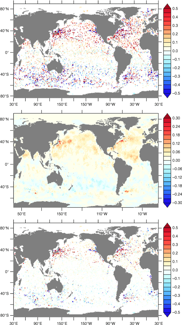
The forecast innovations (the difference between background and observations), increments (the corrections applied to the background to create the analysis) and analysis innovations (the difference between the analysis and the observations) averaged over the period of May 2021 and over 0–20-m depth for temperature are shown in Fig. 2. The pattern of increments resembles the forecast innovations, and the magnitudes of analysis innovations are reduced significantly compared to the forecast innovations. This indicates that the DA system for ACCESS-S2 works as intended in the operational implementation. The performance of the EnOI DA for ACCESS-S2 and its comparison with the 3D-Var DA for ACCESS-S1 is presented in Section 3.
(Top) Monthly mean of 0–20-m depth averaged temperature (°C) forecast innovations, and (middle) increments and (bottom) analysis innovations for May 2021.
The atmospheric component is initialised with a pre-existing atmospheric analysis: ERA-Interim (Dee et al. 2011) for the historical period (1981–2018), and the Bureau’s global four-dimensional variational assimilation analysis (ACCESS-G3; Bureau of Meteorology 2019a) for real-time. The land surface is initialised indirectly through its response to the atmospheric forcing. This is advantageous as it means the initial conditions for soil moisture are realistic (Zhao et al. 2017). The soil moisture was initialised using climatological fields in ACCESS-S1.
2.3. Reanalysis configuration
The DA system described in Section 2.2 was used to produce a reanalysis that covers the period 1981–2018. This was undertaken in parallel over four non-overlapping historical periods. Each of the periods was initialised with a 2-year spin-up integration in order to minimise any shock from the discontinuous run. This method was chosen to reduce the time required to produce the reanalysis. Once the 38 years were complete, the reanalysis was extended to 2019, when the real-time data archive becomes available. From that point onwards, the real-time data sources were assimilated.
The data sources used in the reanalysis are discussed in Section 2.2 and shown in Table 2.
| Reanalysis 1981–2019 | Real-time assimilation 2020 onward | ||
|---|---|---|---|
| Ocean observations source | EN4 | GTS and GDACS | |
| Atmosphere initialisation | ERA-Interim | ACCESS-G3 | |
| SST nudging | Reynolds OISSTv2.1 (to Dec 2013) GAMSSA (2014-onwards) | GAMSSA | |
| SSS nudging | World Ocean Atlas 2013 | World Ocean Atlas 2013 |
2.4. Ensemble generation scheme
The ACCESS-S2 DA system provides a single set of ocean, atmosphere, ice and land fields for a particular day. In order to create an ensemble of predictions for the same start date (a ‘burst’ ensemble), small semi-random perturbations are added to the prognostic atmospheric fields, including the following: zonal (U) and meridional (V) winds and their advected components, potential temperature, specific humidity, density R2, Exner and surface pressure, air density, water vapour mixing ratio and cloud liquid and ice mixing ratios. This process creates 33 distinct members for the real-time forecast, and a variable number for the hindcasts dependent on requirements for a given start-date (see Section 2.5).
The perturbations are derived in the same manner as those for ACCESS-S1 (Hudson et al. 2017). The differences between random 7-day separated reanalysed atmospheric states from ERA-Interim are scaled and then added or subtracted alternately from successive ensemble members. This creates pairs of ensemble members with equal but opposite perturbations.
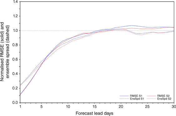
Given that ACCESS-S2 uses the same ensemble perturbation scheme as ACCESS-S1, and similar initialisation of the atmospheric fields (Hudson et al. 2017), we would not expect a significant difference in the large-scale global characteristics of the ensemble forecast for the atmospheric variables. This is reflected in the ensemble root-mean-square error (RMSE) and spread for 500-hPa geopotential heights over the southern hemisphere extratropics (Fig. 3). The tropics and northern hemisphere (not shown) are also very similar between ACCESS-S1 and ACCESS-S2.
Normalised root-mean-square error (RMSE; solid) and ensemble spread (dashed) of daily (00Z) 500-hPa geopotential height over the southern hemisphere (20–90°S) from ACCESS-S2 (red) and ACCESS-S1 (blue). Forecasts were initialised on 1 May for the period 1990–2012 and use nine-member ensembles. The corresponding verification data are from the ERA-Interim reanalysis (Dee et al. 2011), and data are normalised by the standard deviation of ERA-Interim. Before computing the RMSE and ensemble spread, the data are weighted by the square root of the cosine of latitude.
The ensemble that is used for forecast products is based on a combination of time-lagged (combining forecasts from earlier start times) and burst ensembles, as described in Section 2.6.
2.5. Hindcast configuration
A hindcast set is required for:
estimates of forecast skill and reliability;
calibration of the forecasts;
calculation of mean climatologies and thresholds for bias correction;
production of seasonal forecast products.
The design of the ACCESS-S2 hindcast set substantially differs from that of ACCESS-S1. Hindcasts were generated over a longer period of 38 years compared to the 23 years of ACCESS-S1, although the number of ensemble members per year was reduced. ACCESS-S1 had an 11-member ensemble four times per month on the 1st, 9th, 17th and 25th. By contrast, the ACCESS-S2 hindcast configuration employs a time-lagged ensemble approach in which the number of ensemble members is dependent on the start date of the hindcast. This is illustrated by the example in Table 3. The multi-week hindcast integration length is 42 days – the same length as the real-time multi-week integration length. The seasonal hindcast integration length is 279 days. This is longer than the 217 days currently integrated in the real-time forecast system in order to provide support for a potential future increase in real-time forecast length.
| Hindcast start date | Number of members | ||
|---|---|---|---|
| 42-day integration | 279-day integration | ||
| 31 Oct | 9 | 3 | |
| 30 Oct | 9 | 3 | |
| 29 Oct | 3 | 3 | |
| 28 Oct | 3 | 3 | |
| 27 Oct | 3 | 3 | |
| 26 Oct | 3 | 3 | |
| 25 Oct | 3 | 3 | |
| 24 Oct | 3 | 3 | |
| … | |||
| 21 Oct | 3 | 3 | |
| … | |||
| 16 Oct | 9 | 3 | |
| 15 Oct | 9 | 0 | |
| 14 Oct | 9 | 0 | |
| … | |||
| 11 Oct | 3 | 3 | |
| … | |||
| 6 Oct | 3 | 3 | |
| … | |||
| 1 Oct | 9 | 3 | |
| Total members per month | 81 | 39 | |
Ideally the hindcasts would have identical ensemble structure to the real-time forecasts. However, it is not possible to run a full set of seasonal and multi-week ensemble members for every day in the hindcast period due to the prohibitive computing costs. Instead, the hindcast for ACCESS-S2 was designed to be optimally useful for skill assessments, climatology and calibration purposes, while minimising compute and storage requirements.
For a given month (as illustrated in Table 3), the hindcast comprises the following:
Three-member ensembles (out to 279 days) six times per month on the 1st, 6th, 11th, 16th, 21st and 26th to support climatologies and calibration of the real-time system. Real-time forecasts utilise the closest prior climatology date for bias correction or calibration.
A 27-member time-lagged ensemble once per month, valid on the 1st of the month, to support calculation of seasonal skill. This comprises three 279-day ensemble members on 9 successive days (the 1st of the month and the 8 prior days of the previous month).
A 27-member time-lagged ensemble twice per month, valid on the 1st of the month and the 16th of the month, to support calculation of multi-week skill. This comprises nine 42-day ensemble members from 3 successive days: (1) on the 1st of the month plus the 2 days prior and (2) on the 16th of the month plus the 15th and 14th.
The ACCESS-S2 hindcast period is 1981–2018 inclusive. The increase in the length of the hindcast period from ACCESS-S1 is beneficial for forecast calibration and bias correction, increases the statistical robustness of estimates of system performance, and also provides a greater number of cases of low-frequency climate drivers, broadening our understanding of the behaviour of the system in various climatic states. In addition, the larger ensemble in ACCESS-S2 for skill estimates (27 compared to 11) enables a better estimate of the accuracy of forecasts of extreme events (such as top or bottom quintile events). Importantly, moving to a time-lagged ensemble design means that it more closely resembles the real-time system. This provides a truer estimate of the real-time skill, while reducing the overall computing cost of the hindcasts by ~27% in comparison to ACCESS-S1.
2.6. Real-time forecast configuration
The design of the real-time forecast system is the same as that for ACCESS-S1. Every day there is an ensemble of 11 forecasts of seasonal length, and 22 forecasts of multi-week length. The seasonal members are initialised using five pairs of perturbed members and an unperturbed central member, and an additional 11 pairs of perturbed members are used to initialise the multi-week members. Integration length for seasonal and multi-week members is set as 217 and 42 days respectively. The seasonal integration length provides six full calendar-month averages of the forecast variables. The first 6 weeks of the seasonal members are included in the multi-week ensemble to give a total of 33 members.
Forecasts are run every day in real-time. As for ACCESS-S1, the Bureau’s ACCESS-S2 climate outlook products are based on a 99-member ensemble which is a combination of burst and time-lagged ensemble members (i.e. 9 successive days of forecasts for seasonal products and 3 successive days of forecasts for multi-week products).
2.7. Forecast post-processing
The forecast post-processing suites are part of the real-time system in both ACCESS-S1 (Bureau of Meteorology 2019b) and ACCESS-S2, although there is additional functionality in ACCESS-S2.
In summary, the post-processing in both ACCESS-S1 and S2:
Creates anomalies (i.e. bias correction) by removing a lead-time dependent model climatology from the hindcasts.
Creates calibrated 5-km datasets of key atmospheric variables over Australia. The variables include rainfall, minimum and maximum temperature, vapour pressure, evapotranspiration, solar exposure and 10-m windspeed. The calibration technique is based on quantile–quantile matching (Wilk and Gnanadesikan 1968) and is the same as was used for ACCESS-S1.
Combines the daily lagged forecasts into 99-member ensembles and calculates ensemble means.
Creates temporal averages (weekly, monthly or seasonal) from the daily data.
In ACCESS-S2, the functionality is increased to include new modules to support the operational forecast products e.g. calculation of spatial averages and indices such as El Niño–Southern Oscillation (ENSO) indices, Indian Ocean Dipole (IOD), Madden–Julian Oscillation (MJO) and the Southern Annular Mode (SAM), and production of probabilities of above or below median or top or bottom quintile etc. Centralising this product generation code increases efficiencies, reduces duplication of effort and reduces the chance of errors – especially as the demand for more complex forecast products is increasing. The code is modular and facilitates the efficient addition of new forecast products in the future.
Further details of the operational forecast post-processing can be found in Bureau of Meteorology (2019b). In addition, the research post-processing suite (which includes the operational modules and more) is described in de Burgh-Day et al. (2020).
3.Reanalysis results and evaluation
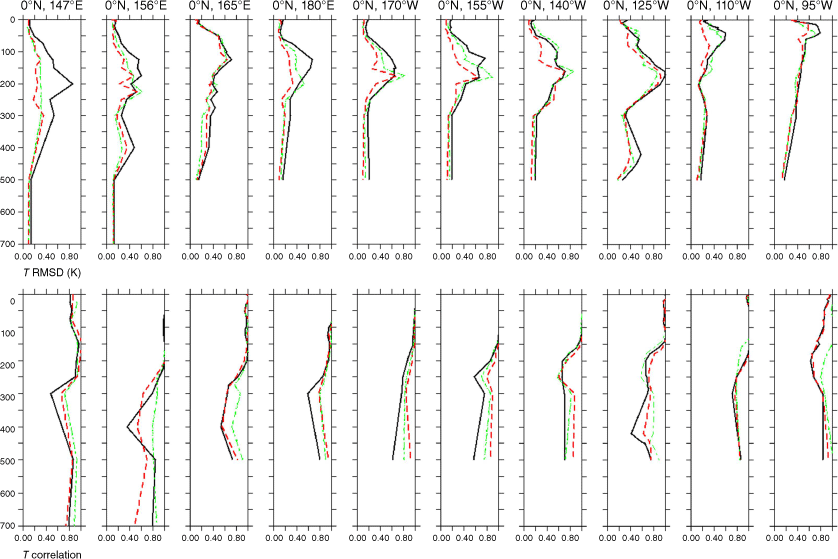
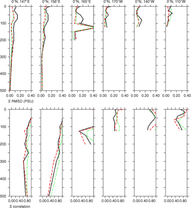
The ACCESS-S2 reanalysis covers the period 1981–2018, but comparisons with ACCESS-S1 need to address the common reanalysis period (1990–2014; note that although the ACCESS-S1 hindcast period only extends to 2012, an additional 2 years of the reanalysis were available for this comparison). The 25-year common reanalysis period is compared with both assimilated and independent observations, including in situ temperature, salinity and velocity observations and the EN4 objective analysis. Comparisons with temperature profiles measured by the TAO/TRITON array are shown in Fig. 4. Profiles of root mean square difference (RMSD) and correlation are shown for different longitudes along the equator at locations of the TAO/TRITON moorings. Generally, ACCESS-S1 has slightly smaller RMSD values and larger correlations than ACCESS-S2, although the results are similar. Both are very close to the results of EN4 analysis at different locations. The salinity profiles in Fig. 5 display a similar congruence between the three systems.
Profiles of (top) RMSD (K) and (bottom) correlation with depth (m; y-axis) between temperature from TAO/TRITON monthly means and from ACCESS-S2 (solid black), ACCESS-S1 (dashed red) and EN4 analysis (dashed green) over the period 1990–2014 along the equator at different longitudes (see titles for each column).
Profiles of (top) RMSD (PSU) and (bottom) correlation with depth (m; y-axis) between salinity from TAO/TRITON monthly means and from ACCESS-S2 (solid black), ACCESS-S1 (dashed red) and EN4 analysis (dashed green) over the period 1990–2014 along the equator at different longitudes (see titles for each column).
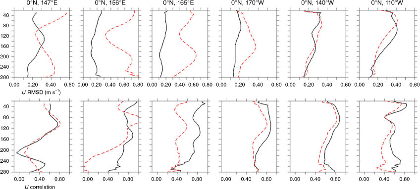
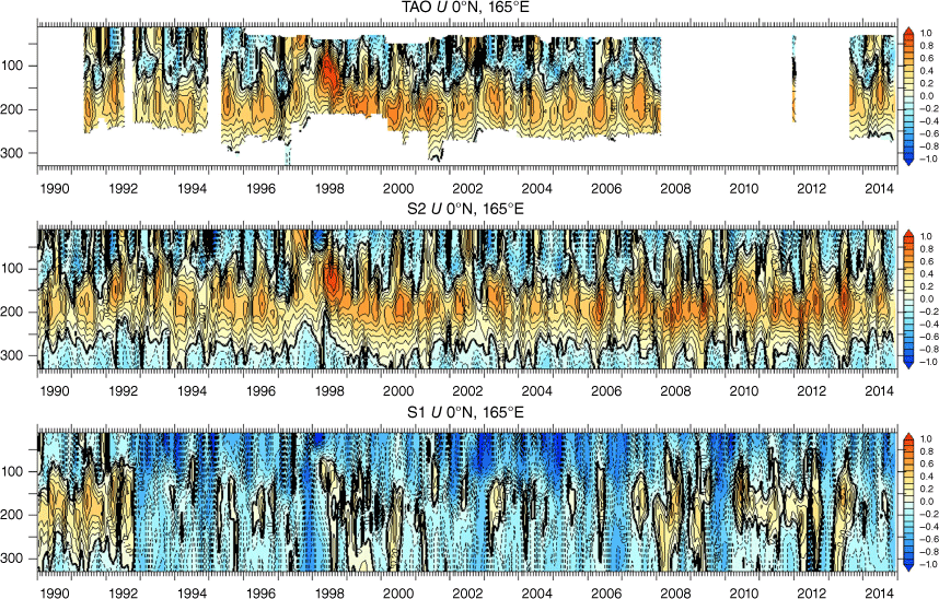
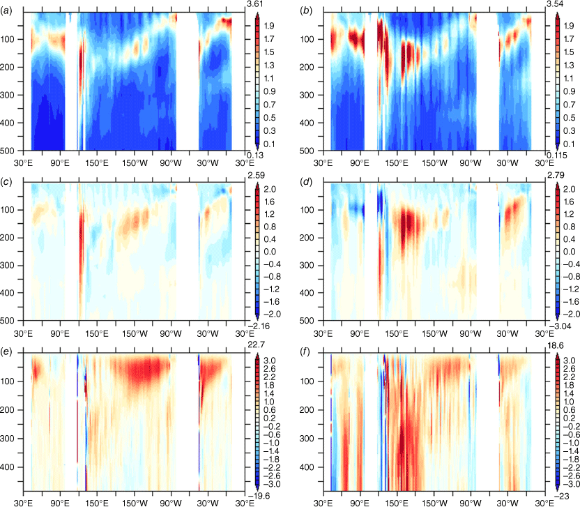
However, significant differences between the systems are found in zonal velocity profiles, measured by TAO acoustic Doppler current profiler (ADCP; Fig. 6). Here ACCESS-S1 shows larger RMSD values and smaller correlations than ACCESS-S2. This is also evident from the monthly mean ocean zonal (u)-current with depth at 0°N and 165°E from observations (ADCP TAO/TRITON) and the ACCESS-S2 and ACCESS-S1 reanalyses (Fig. 7). ACCESS-S1 ocean currents are relatively inaccurate, with ACCESS-S2 closer to independent observations. This is possibly due to more dynamically consistent increments in ACCESS-S2. ACCESS-S1 may also be overfitting to the assimilated observations, or the assimilation of altimeter data (not used in ACCESS-S2) may be having a detrimental effect on the subsurface ocean currents. To investigate this, differences between reanalyses and the EN4 analysis are analysed. The RMSD and the mean of the difference in temperature between each reanalysis and EN4, and the corresponding annual mean equatorial vertical velocities from each reanalysis are shown in Fig. 8. ACCESS-S1 has significantly larger RMSD values (Fig. 8b) and mean temperature offsets (Fig. 8d) in the vicinity of the thermocline in equatorial oceans compared to ACCESS-S2 (Fig. 8a, c). The most significant discrepancy between ACCESS-S1 and EN4 is in the western Pacific and corresponds with a spurious vertical upward velocity in the deep ocean (up to 2000 m deep, Fig. 8f shows the results for top 500 m). The subsurface warm bias in the equatorial western Pacific is likely caused by the assimilation of altimeter data in ACCESS-S1 and a lack of sufficient in situ observations to constrain the subsurface field. This can cause an imbalance and lead to initialisation shock where spurious equatorial waves and vertical velocities are triggered. The equatorial waves and vertical velocities can degrade the performance of the ocean model and lead to unrealistic subsurface temperature and current fields (e.g. Waters et al. 2017; Park et al. 2018; Gasparin et al. 2021). The equatorial Indian Ocean and Atlantic Ocean in ACCESS-S1 seem to have similar imbalances. These results suggest that the ACCESS-S2 DA performs better than ACCESS-S1 in the equatorial oceans due to more dynamically consistent increments.
Profiles of (top) RMSD (m s−1) and (bottom) correlation with depth (m; y-axis) between zonal currents from TAO/TRITON ADCP monthly means and from ACCESS-S2 (solid black) and ACCESS-S1 (dashed red) over the period 1990–2014 along the equator at different longitudes (see titles for each column).
Monthly mean ocean zonal currents (m s−1) with depth (m; y-axis) at 0°N and 165°E for the period of 1990–2014 (x-axis) from (top) observations (TAO/TRITON ADCP), (middle) the ACCESS-S2 reanalysis and (bottom) the ACCESS-S1 reanalysis.
Equatorial longitude-depth (m) sections from (a, c, e) ACCESS-S2 and (b, d, f) ACCESS-S1 for (a, b) RMSD (°C) and (c, d) mean (°C) temperature differences between reanalyses and EN4 analysis. (e, f) Mean vertical velocity (10−5 m s−1) averaged over 1990–2014.
The global correlation of upper ocean heat (T300) and salinity (S300) content with EN4 from each reanalysis over the period 1990–2014 is shown in Fig. 9. The distribution of T300 correlations from ACCESS-S2 (Fig. 9a) is similar to that of ACCESS-S1 (Fig. 9b), showing high correlations (>0.9) in most of the equatorial Pacific, and parts of the equatorial Indian, equatorial Atlantic, northern Pacific and northern Atlantic Oceans. The global mean of T300 correlation coefficients is 0.57 for ACCESS-S2 and 0.58 for ACCESS-S1. ACCESS-S2 produces higher correlations in the equatorial oceans, particularly in the western Pacific. The average of correlations within 10°S–10°N is 0.81 for ACCESS-S2 and 0.78 for ACCESS-S1. The distribution of S300 correlations from ACCESS-S2 (Fig. 9c) with EN4 is also similar to ACCESS-S1 (Fig. 9d). The area average of S300 correlation within 10°S–10°N band is 0.57 for ACCESS-S2 and 0.54 for ACCESS-S1, whereas the global average is 0.36 for ACCESS-S2 and 0.39 for ACCESS-S1. These results suggest that the ACCESS-S2 performs better in equatorial oceans than ACCESS-S1, whereas ACCESS-S1 outperforms ACCESS-S2 in the subtropical to high latitude oceans.
Correlation of (a, b) T300 and (c, d) S300 against EN4 in 1990–2014 for (a, c) ACCESS-S2 and (b, d) ACCESS-S1.
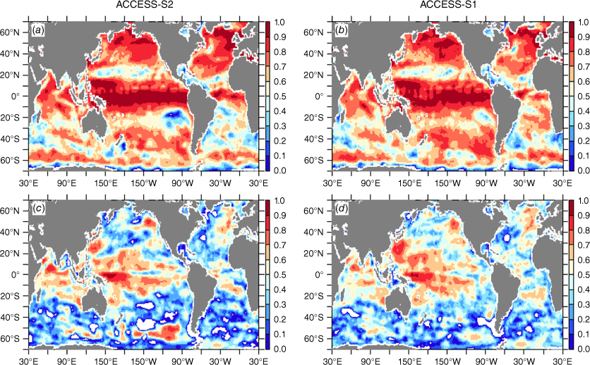
The correlation coefficients of S300 from both reanalyses are generally lower than those of T300. This is mainly due to the paucity of salinity observations, particularly prior to the deployment of Argo profiling floats in the early 2000s, leading to a large analysis uncertainty in S300.
Fig. 10 shows monthly time series (filtered with a 13-month running mean) of T300 and S300 averaged in eastern equatorial Pacific (150–90°W, 5°S–5°N), western equatorial Pacific (150°E–170°W, 5°S–5°N), equatorial Indian Ocean (30–120°E, 10°S–10°N), equatorial Atlantic (60°W–20°E, 10°S–10°N) and global ocean (0–360°E, 90°S–90°N). Both ACCESS-S2 and ACCESS-S1 reanalyses are highly consistent in T300 with EN4 in the eastern (Fig. 10a) and western (Fig. 10c) equatorial Pacific Ocean. This is essential for a skilful ENSO forecast as heat contents in both eastern and western Pacific play key roles in ENSO dynamics. This is mostly attributable to the TAO/TRITON array providing good coverage of temperature observations in the tropical Pacific in the early 1990s, and Argo data becoming available from the early 2000s. It is notable that ACCESS-S1 has a persistent warm offset from EN4 after 1992 in the western equatorial Pacific (Fig. 10c), which is related to the altimeter assimilation applied after 1992 and the warm bias and the spurious vertical velocities (shown in Fig. 8) as discussed above. This helps explain why a better ENSO prediction skill is achieved with ACCESS-S2 (see below) compared to ACCESS-S1.
Time series of 13-month running means of T300 (left column, °C) and S300 (right column, PSU) averaged in regions of (a, b) eastern equatorial Pacific (150–90°W, 5°S–5°N), (c, d) western equatorial Pacific (150°E–170°W, 5°S–5°N), (e, f) equatorial Indian Ocean (30–120°E, 10°S–10°N), (g, h) equatorial Atlantic (60°W–20°E, 10°S–10°N) and (i, j) global (0–360°E, 90°S–90°N) from ACCESS-S2 (black), ACCESS-S1 (red) and EN4 (green).
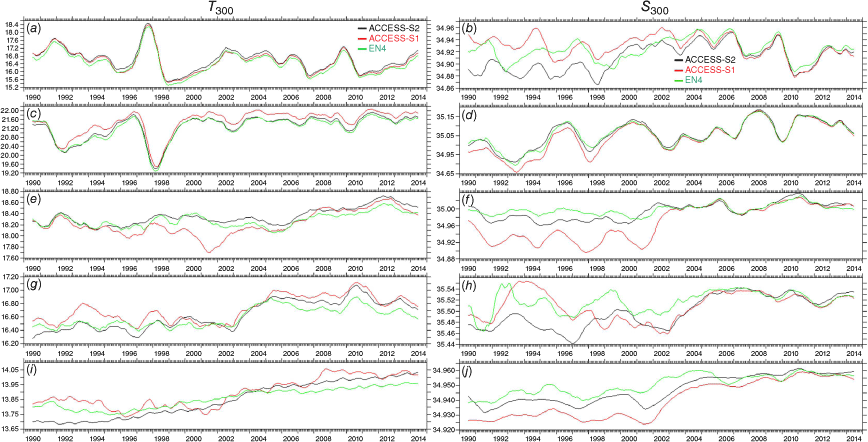
The T300 is moderately consistent between ACCESS-S2 and EN4 in both equatorial Indian (Fig. 10e) and Atlantic Oceans(Fig. 10g). The ACCESS-S1 reanalysis has a significant cold offset in the equatorial Indian Ocean during 1996–2002 when the temperature observations are sparse. The offsets diminish significantly c. 2003 with the implementation of Argo and RAMA observational platforms (Fig. 10e). In the equatorial Atlantic Ocean, the ACCESS-S1 reanalysis has a significant warm offset before 1998 that reduces until increasing again after 2005 (Fig. 10g). The PIRATA moorings were implemented on the equatorial Atlantic Ocean c. 1998, which seems to have a significant influence on the offset. However, there is an unexpected general warm bias in both ACCESS-S1 and ACCESS-S2 after 2005 (Fig. 10g), indicating large uncertainties in the mean T300 in the equatorial Atlantic. To reduce these uncertainties, improvement in other components of the assimilation system, such as surface fluxes, model physics and DA schemes, and an increase in model resolution, may be needed in addition to enhancing ocean observing systems. The global mean of T300 (Fig. 10i) shows ACCESS-S2 has a continued upward global warming trend for 1995–2014, coinciding with EN4, whereas ACCESS-S1 has more fluctuations on the warm trend. Both EN4 and ACCESS-S1 show a cooling for 1992–1994.
The change of the observation system has a significant effect on S300 variabilities shown in the right panel of Fig. 10. During the entire period of 1990–2014, ACCESS-S2 is closer to EN4 than ACCESS-S1 in the equatorial western Pacific Ocean (Fig. 10d), Indian Ocean (Fig. 10f) and global average (Fig. 10j). There are significant offsets relative to EN4 before the early 2000s in most areas for both systems, indicating that there were insufficient salinity observations to constrain the salinity fields of both the model and the objective analysis. There is a distinct change after Argo deployment, with both reanalyses reaching good agreement with the EN4 objective analysis in all areas.
The ocean DA system also has an impact on the ocean biases in model forecasts. The subsurface temperature bias is calculated with World Ocean Atlas 2018 data (Locarnini et al. 2018). Fig. 11 shows the temperature bias with depth along the equator for lead times of 0 months (i.e. first month of the forecast) and 4 months (i.e. fifth month of the forecast) for all start months. ACCESS-S1 has a warm bias in the subsurface of the western Pacific in the initial conditions (reanalysis) (Fig. 8d), but it cools rapidly during the first month of the forecast (lead month 0; Fig. 11) due to the strong upwelling (Fig. 8f) caused by deficiencies of the NEMOVAR DA. By contrast, ACCESS-S2 has a much smaller drift towards cooler conditions (Fig. 8c, 11) due to much weaker upwellings (Fig. 8e) in this region. The sub-surface cold bias propagates eastward from the western to the eastern Pacific along the path of the thermocline depth, resulting in a cold bias near the surface in the eastern Pacific after 3 months of the forecast initialisation (not shown) and still visible after 5 months (Fig. 11). This cold tongue bias is also evident in the SST bias (Fig. 12) and is reduced in ACCESS-S2.
Temperature biases averaged over 2°S–2°N along the equator for (left) ACCESS-S2, (middle) ACCESS-S1 and (right) their differences at 0-month (first month of the forecast, top) and 4-month lead times (fifth month of the forecast, bottom). The World Ocean Atlas 2018 data are used here to calculate the model biases (Locarnini et al. 2018).

SST biases for (left) ACCESS-S2, (middle) ACCESS-S1 and (right) their differences in (top) the first month of the forecast (0-month lead time) and (bottom) the fifth month of the forecast (4-month lead time). The SST biases are computed with respect to Reynolds OI SST data (Reynolds et al. 2002).

The weakly coupled DA of ACCESS-S2 also improves the initialisation of the land surface. In ACCESS-S1, soil moisture was initialised with climatological fields, which negatively affected the skill, particularly for maximum temperature in the first month of the forecast during late autumn and winter (Hudson et al. 2017; Zhao et al. 2017). By contrast, in ACCESS-S2, the interannual variation in the soil moisture initial conditions is realistic since it responds to the atmospheric forcing during the DA. The impact of this on the skill of the ACCESS-S2 forecasts will be shown in the following section.
4.Forecast performance
In this section, all evaluation between ACCESS-S1 and ACCESS-S2 hindcasts has been performed over the common hindcast period of 1990–2012, using comparable ensemble sizes. Unless otherwise mentioned, for monthly and seasonal forecasts the 11-member ensemble initialised on the first of the month is used from ACCESS-S1. This is compared to the nine-member ensemble from ACCESS-S2 which is also valid for the first of the month but comprises three ensemble members on 3 successive days (i.e. a time-lagged ensemble initialised on the 1st, t − 1 and t − 2 days; see Section 2.5). For the multi-week forecasts, forecasts initialised twice per month are used, i.e. on the 1st and 16th (17th for ACCESS-S1). The ensemble size on these start dates is 11 members for ACCESS-S1 and nine for ACCESS-S2.
4.1. Climate drivers
The SST anomaly (SSTA) skill drops off rapidly outside the tropics with lead time (Fig. 13: correlation skill shown for all forecast start months). In the first month of the forecast (LT0) there are indications that ACCESS-S2 has higher skill than ACCESS-S1 over the tropics, particularly for the western Pacific, western Indian and Atlantic Oceans. However, ACCESS-S2 is worse than ACCESS-S1 in the high southern latitudes. This is likely related to the lack of direct sea-ice assimilation in ACCESS-S2. In ACCESS-S2, the sea-ice responds to the coupled forcing of the model during the DA process (see Section 2.2). By contrast, the FOAM analysis used in ACCESS-S1 (Blockley et al. 2014) directly assimilates sea-ice observations. After 5 months of the forecast, ACCESS-S2 SST skill is still generally higher than ACCESS-S1 in the tropics as well as in some key regions of the extratropics such as the South Pacific Convergence Zone. These results are for all forecast start months. Seasonally specific results are examined below with respect to ENSO and IOD.
Correlation skill of predicting SSTA for (left) ACCESS-S2, (middle) ACCESS-S1 and (right) their differences at 0- and 4-month lead times. The significant correlations (at the 5% level with one-tailed Student’s t-test) are shaded. Forecasts are verified against Reynolds OI SST data (Reynolds et al. 2002).

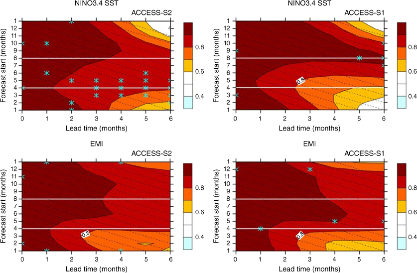
ENSO is the most prominent driver of climate variability and predictability on seasonal timescales, including for Australian climate (e.g. Wang and Hendon 2007; Risbey et al. 2009; Cai et al. 2011; White et al. 2014; Lim and Hendon 2015a; Marshall et al. 2022). The NINO3.4 and El Niño Modoki (EMI; Ashok et al. 2007) Indices are used for monitoring and predicting two different types of ENSO. NINO3.4 is the area-averaged SSTA over the central–eastern Pacific (5°N–5°S, 170–120°W), which commonly represents cold-tongue, eastern Pacific, canonical or traditional ENSO events. The EMI measures variability of ENSO events whose maximum SST anomalies are found over the dateline. The warm phase of this type of ENSO is referred to as warm-pool, dateline, central Pacific or Modoki El Niño (Hendon et al. 2009 and references therein). The index is computed by the difference between the central Pacific SST anomalies (10°N–10°S, 165–220°E) and the sum of the half magnitudes of the far eastern (15°S–5°N, 70–110°W) and western Pacific (10°S–20°N, 125–145°E) SST anomalies (Ashok et al. 2007). Fig. 14 shows correlation skill of predicting the NINO3.4 index (top) and the EMI (bottom) as a function of forecast start month (y-axis) and lead time (x-axis) for each system. There is a clear improvement in skill for forecasts of canonical or traditional ENSO initialised in late summer and autumn (February–May) represented by the NINO3.4 index (Fig. 14 upper panels). This is a pleasing result, since it is a challenging time of year for ENSO predictions by dynamical and statistical models alike (Barnston et al. 2012), with difficulty in predicting the development or decay of ENSO through the so-called boreal spring predictability barrier (Webster 1995). ACCESS-S2 appears to also provide more skilful forecasts of warm-pool El Niño events (EMI) at longer lead times when forecasts are initialised in austral summer and early autumn, but these improvements are not statistically significant. Skill at other times of the year is similar between the two systems, although perhaps slightly worse at longer lead times beyond 3 months in ACCESS-S2 for forecasts initialised c. August and later for the NINO3.4 index, which are associated with a weak warming trend in ACCESS-S2 as opposed to weak cooling trends in ACCESS-S1 and the observations.
Correlation skill of predicting (upper) the NINO3.4 SST index and (lower) the El Niño Modoki Index. The y-axis denotes forecast start months, and the x-axis denotes forecast lead time in months. The diagonal dashed lines indicate constant verification months. The cyan asterisks on the ACCESS-S2 (S1) panel indicate where the ACCESS-S2 (S1) forecasts are significantly better than the ACCESS-S1 (S2) forecasts from a test which resamples 10 000 times with replacement. We consider the hindcast skill of one version (test version) is significantly better than that of the other (reference version) if the 90th percentile threshold of the high tail of the probability density function of the test version is greater than the 99th percentile threshold of that of the reference version. The white horizontal lines are the references for skill comparison between ACCESS-S1 and -S2 discussed in the main text. Forecasts are verified against Reynolds OI SST data (Reynolds et al. 2002).
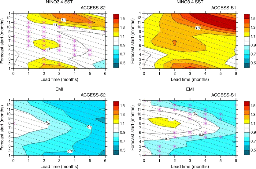
ACCESS-S1 predicts traditional ENSO events (NINO3.4) with amplitudes that are overly strong (Hudson et al. 2017) (Fig. 15), which is a common bias in dynamical models (Barnston et al. 2012). The ENSO amplitude is measured by the standard deviation of the magnitude of the predicted NINO3.4 (upper panels) and EMI (lower panels) indices, expressed as a ratio to the observed standard deviation (i.e. a ratio of one indicates a perfect match between the model and observations). The stronger than observed amplitude for forecasts of NINO3.4 from ACCESS-S1 is evident in Fig. 15, with ratios greater than one for most start dates and lead times. ACCESS-S2 forecasts of the amplitude of NINO3.4 are much more realistic. A similar result is found for NINO3 SSTs (not shown). However, the predicted amplitude of warm-pool El Niño events (as given by the EMI) by ACCESS-S1 is generally realistic for the seasons when they develop (July–December) (Fig. 15 lower panels), but the amplitude of the EMI predicted by ACCESS-S2 is too damped and worse than ACCESS-S1, particularly at longer lead times.
(Upper) Ratio of the standard deviation of the forecast NINO3.4 SST index to that of the observed and (lower) the same as the upper panels except the El Niño Modoki Index (EMI). The diagonal dashed lines indicate constant verification months. The magenta asterisks on the ACCESS-S2 (or ACCESS-S1) panel indicate where the ACCESS-S2 (or ACCESS-S1) forecasts are significantly better than the ACCESS-S1 (or ACCESS-S2) forecasts in predicting the amplitudes of the predict and indices, as estimated from a test which resamples 10 000 times with replacement. For forecasts of the amplitudes, we consider the hindcast skill of one version (test version) is significantly better than that of the other (reference version) if the 90th (10th) percentile threshold of the high (low) tail of the probability density function (PDF) of the test version is closer to the observation than the 99th (1st) percentile threshold of the high (low) tail of the PDF of the reference version. Forecasts are verified against Reynold OI SSTs (Reynolds et al. 2002).
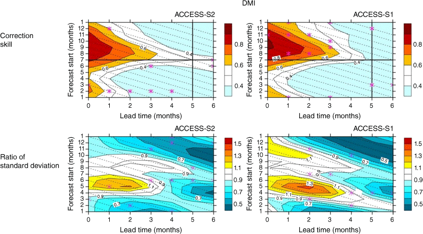
Low-frequency coupled ocean–atmosphere variations in the tropical Indian Ocean, typically quantified by the IOD, are also an important driver of variability and predictability of Australian climate (e.g. Risbey et al. 2009; Cai et al. 2011; White et al. 2014; Lim et al. 2021a; Marshall et al. 2022). The IOD is monitored by the Dipole Mode Index (DMI) which is the difference in SSTA between the western (10°S–10°N, 50–70°E) and eastern (10°S–0°, 90–110°E) Indian Ocean (Saji et al. 1999). The differences in skill between ACCESS-S2 and ACCESS-S1 for forecasts of the IOD are relatively small (Fig. 16 upper panels). There is a slight improvement in skill at long lead times in ACCESS-S2 when the forecasts are initialised in June–August. However, there is a decrease in skill at the shortest lead times in ACCESS-S2 compared to ACCESS-S1 for the IOD peak season (September–October). The predicted amplitude of the IOD is more realistic in ACCESS-S2 for the winter but substantially damped for late spring at lead times of longer than 3 months compared to that predicted by ACCESS-S1 (Fig. 16 lower panels).
(Upper) Correlation skill of predicting the Indian Ocean Dipole Mode Index (DMI) and (lower) ratio of the standard deviation of the forecast DMI to that of the observed. The diagonal dashed lines indicate constant verification months. The magenta asterisks indicate significant skill difference as described in the captions of Fig. 14, 15. The black solid lines in the upper panels are the references for skill comparison between ACCESS-S1 and S2 discussed in the main text. Forecasts are verified against Reynold OI SSTs (Reynolds et al. 2002).
The MJO is a key driver of predictability on multi-week timescales (e.g. Wheeler et al. 2009; Marshall et al. 2011, 2014, 2021, 2022; Wang and Hendon 2020). The MJO is monitored using the real-time multivariate MJO (RMM) indices from Wheeler and Hendon (2004). The two RMM indices, RMM1 and RMM2, provide a measure of the strength and phase of the MJO. They are the principal components of the leading pair of eigenvectors derived from a combined empirical orthogonal function (EOF) analysis of equatorially averaged outgoing longwave radiation and zonal wind at 200 and 850 hPa. This leading pair of EOFs describes the eastward propagation of the combined convection and zonal wind that characterises the MJO.
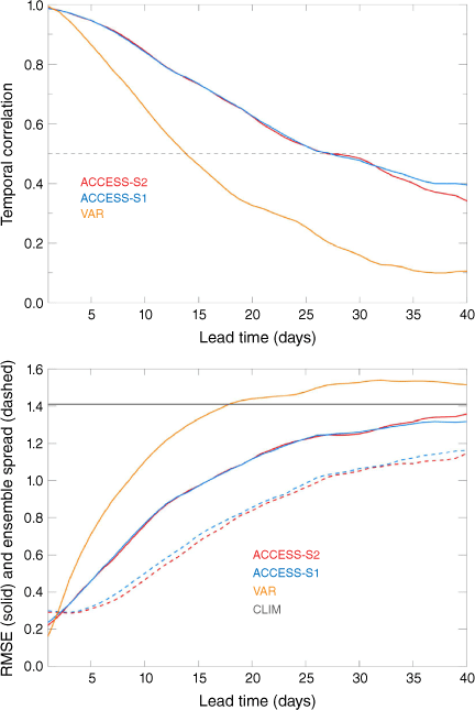
Forecast skill, RMSE and ensemble spread of the RMM bivariate MJO index with lead time is basically the same for both systems (Fig. 17). This is not surprising, since the main changes between ACCESS-S2 and ACCESS-S1 (ocean and land initialisation) are unlikely to have a big effect on the MJO. ACCESS-S2 produces skilful forecasts of the MJO out to ~30-day lead time (Fig. 17), surpassing the 14-day limit of skill achieved with the vector autoregressive ‘VAR’ bivariate persistence forecast of the MJO (Maharaj and Wheeler 2005). The level of skill achieved by ACCESS-S2 is among the best of the skill recorded from other international systems, which have a lead-time range of 12–36 days (Lim et al. 2018). Specifically, ACCESS-S2 produces the second highest level of skill behind the ECMWF model (36 days) and ahead of POAMA2 (28 days; the predecessor to ACCESS-S) and both the UKMO and NCEP (26 days) (Lim et al. 2018). This result highlights the Bureau’s multi-week to seasonal prediction system suite as a consistent top performer for MJO prediction.
(Upper) Correlation and (lower) root-mean-square error (RMSE; solid lines) of the predicted bivariate RMM index for the ensemble mean forecasts from ACCESS-S2 (red), ACCESS-S1 (blue) and for the ‘VAR’ statistical model developed by Maharaj and Wheeler (2005) (orange), as a function of lead time (days) for all forecast start months in 1990–2012. Also shown (lower) is the bivariate RMSE for a reference forecast using climatology (CLIM; grey) and the bivariate ensemble spread for ACCESS-S2 and ACCESS-S1 (dashed lines). Forecasts are verified against ERA-Interim (Dee et al. 2011).
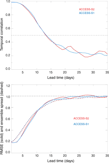
The SAM has also been identified as a driver of Australian climate on multi-week and seasonal timescales (Hendon et al. 2007; Marshall et al. 2012, 2014, 2022; Lim and Hendon 2015b; Lim et al. 2016, 2019, 2021b). The SAM is represented by the variability of mean sea level pressure (MSLP) around the southern mid-latitudes. The index is calculated by projecting daily MSLP anomalies from the NCEP–NCAR reanalysis (Kalnay et al. 1996) onto the leading EOF of observed monthly mean MSLPs between 25 and 75°S. For both ACCESS-S1 and ACCESS-S2, the predicted MSLP anomalies from each model ensemble member are projected onto the observed EOF to calculate their respective indices (see Marshall et al. 2012 for details). As for the MJO, the skill (RMSE) and spread for forecasts of the SAM on multi-week timescales from the two systems are very similar (Fig. 18). Both can predict the SAM out to ~16-day lead time (given by correlations greater than 0.4 and RMSEs less than that of a climatological forecast). Both ACCESS-S1 and ACCESS-S2 have ensembles that are slightly over-dispersed (the spread is greater than the error) in the first 10 days of the forecast.
(Upper) Correlation and (lower) root-mean-square error (RMSE; solid lines) of the predicted SAM index for the ensemble mean forecasts from ACCESS-S2 (red) and ACCESS-S1 (blue) as a function of lead time (days) for all forecast start months in 1990–2012. (Lower) Ensemble spread is also shown (dashed lines). Forecasts are verified against the NCEP-NCAR Reanalysis (Kalnay et al. 1996).
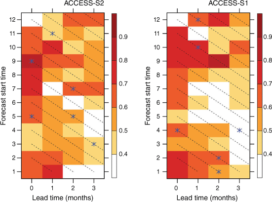
Likewise, seasonal SAM skill in ACCESS-S2 is similar to ACCESS-S1, although there are some notable improvements for forecasts initialised in May–August across different lead times and reduced skill for the October–December and November–January verification seasons at short lead times (Fig. 19).
Correlation skill of seasonal mean SAM. The dashed diagonal lines indicate consistent verification seasons following forecast initialisation. The blue asterisks indicate the significant skill difference as estimated by the resampling test with replacement as described in Fig. 14. Forecasts are verified against the observed SAM index derived from JRA-55 reanalysis (Kobayashi et al. 2015).
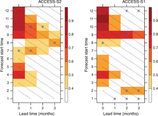
Antarctic stratospheric polar vortex variability has received increased attention since 2019 when a rare extreme stratospheric polar vortex weakening event occurred (Lim et al. 2021b). This resulted in the record strong negative amplitude of the SAM in the last 40 years and significantly contributed to the devastating bushfires along the eastern seaboards of southern Queensland and New South Wales during October–December 2019 (Lim et al. 2021b). Fig. 20 shows that both ACCESS-S1 and ACCESS-S2 have reasonably good skill (i.e. significant at the 95% confidence level) at up to 3 months of lead time to predict the stratospheric polar vortex over Antarctica during spring to early summer seasons when the vortex variability is the greatest and its anomalous signal is coupled down to the surface. Here, the Antarctic stratospheric polar vortex is monitored by the zonally averaged zonal wind anomalies at the 10-hPa level at 60°S. Overall skill in ACCESS-S2 is comparable to that of ACCESS-S1, which is highly competitive with other international models (Lim et al. 2021b), although it is encouraging to see indications of improved skill for the spring to early summer seasons when forecasts are initialised in July and August.
As for Fig. 19 except the skill to predict seasonal mean stratospheric polar vortex over Antarctica, which is monitored by the zonal mean zonal wind anomalies at the 10-hPa level at 60°S.
4.2. Skill for Australian climate
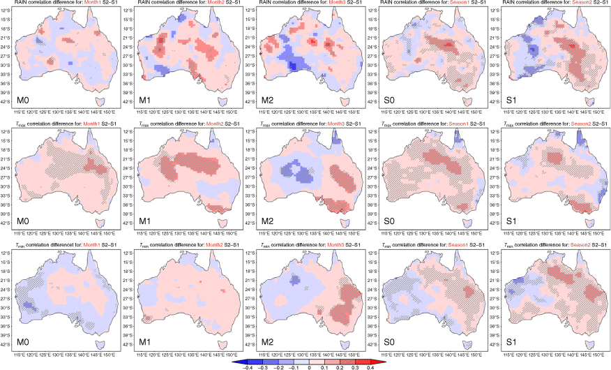
Fig. 21 is a high-level summary of skill averaged over Australia for all times of year and different lead times for rainfall, maximum temperature (Tmax) and minimum temperature (Tmin) forecasts from ACCESS-S1 and ACCESS-S2 over the period 1990–2012. This analysis obscures any regional and seasonal differences in skill but shows that ACCESS-S2 is very similar to ACCESS-S1 in overall performance, especially on multi-week timescales. The biggest signal is likely the increase in skill for Tmax on monthly and seasonal timescales in ACCESS-S2. The difference in monthly or seasonal skill between ACCESS-S2 and ACCESS-S1 for rainfall and temperature for all seasons is shown spatially in Fig. 22 (red indicates ACCESS-S2 is better). Again, this shows that, overall, the skill is similar between the two systems, perhaps slightly better in ACCESS-S2.
Correlation skill averaged over Australia for all times of year for (left) rainfall, (middle) maximum temperature and (right) minimum temperature anomalies from ACCESS-S1 (green bars) and ACCESS-S2 (red bars) for the period 1990–2012. The x-axis is the forecast verification period at different lead times for the multi-week forecasts i.e. WK1 (week 1), WK2 (week 2), WK3 (week 3), WK4 (week 4), WK12 (weeks 1 and 2), WK23 (weeks 2 and 3) and WK34 (weeks 3 and 4) of the forecast, and the monthly or seasonal forecasts for M0 (first month of the forecast, i.e. 0-month lead time), M1 (i.e. second month of the forecast lead time, i.e. 1-month lead time), M2 (third month of the forecast, i.e. 2-month lead time), S0 (3-month mean forecast at 0-month lead time), and S1 (3-month mean forecast at 1-month lead time). The multi-week results are based on 11-member ensembles from ACCESS-S1 and nine-member ensembles from ACCESS-S2 initialised twice per month: on the 1st and the 16th (the 17th for ACCESS-S1). The monthly and seasonal results are based on time-lagged ensembles valid for the 1st of the month start dates: for ACCESS-S1 it is a 22-member time-lagged ensemble comprising 11-member ensembles from the 1st and prior 25th; and for ACCESS-S2 it is a 21-member ensemble comprising three-member ensembles from the 1st and 6 consecutive days prior. Verification data are the Australian Water Availability Project (AWAP) gridded datasets (Jones et al. 2009).

The difference in correlation skill for all times of year for (top) rainfall, (middle) maximum temperature and (bottom) minimum temperature anomalies between ACCESS-S2 (S2) and ACCESS-S1 (S1) for monthly and seasonal forecasts at different lead times (columns). The lead times (M0, M1, M2, S0 and S1) are as defined in Fig. 21. Verification data are the Australian Water Availability Project (AWAP) gridded datasets (Jones et al. 2009). Red colours indicate higher correlations in ACCESS-S2. The hatched lines represent correlation differences that are significantly different, as determined by bootstrapping. The 23-year hindcast was resampled (pairwise with replacement) 1000 times at each grid point. The 95% confidence intervals of the correlation difference was calculated (using a percentile approach) and if the interval did not include zero, the correlation difference was deemed significant.
One of the advances of ACCESS-S2 over ACCESS-S1 is the realistic initialisation of soil moisture. In ACCESS-S1, soil moisture was initialised with climatological fields, which negatively affected the skill, particularly for Tmax in the first month of the forecast and in the winter-half of the year. Fig. 23 shows the correlation skill for forecasts of May (from 1 May) for ACCESS-S1 and ACCESS-S2. There is a clear improvement in the skill over northern, eastern and western Australia in ACCESS-S2. It is pleasing to note that these improvements are as expected based on prior sensitivity experiments investigating the impact of soil moisture initialisation on forecast skill (Hudson et al. 2017; Zhao et al. 2017).
Correlation skill of forecasts of maximum temperature anomalies for May from (a) ACCESS-S1 and (b) ACCESS-S2 at 0-month lead time, and (c) the difference in the correlation between ACCESS-S2 and ACCESS-S1. Forecasts were initialised on 1 May for the period 1990–2012 and based on 21/22-member time-lagged ensembles (as described in Fig. 21). Verification data are the Australian Water Availability Project (AWAP) gridded datasets (Jones et al. 2009). The black dashed lines on (a, b) indicate significant correlations at the 5% level (t-test). The hatched lines on (c) represent the significant correlation differences, determined by bootstrapping (as described for Fig. 22).

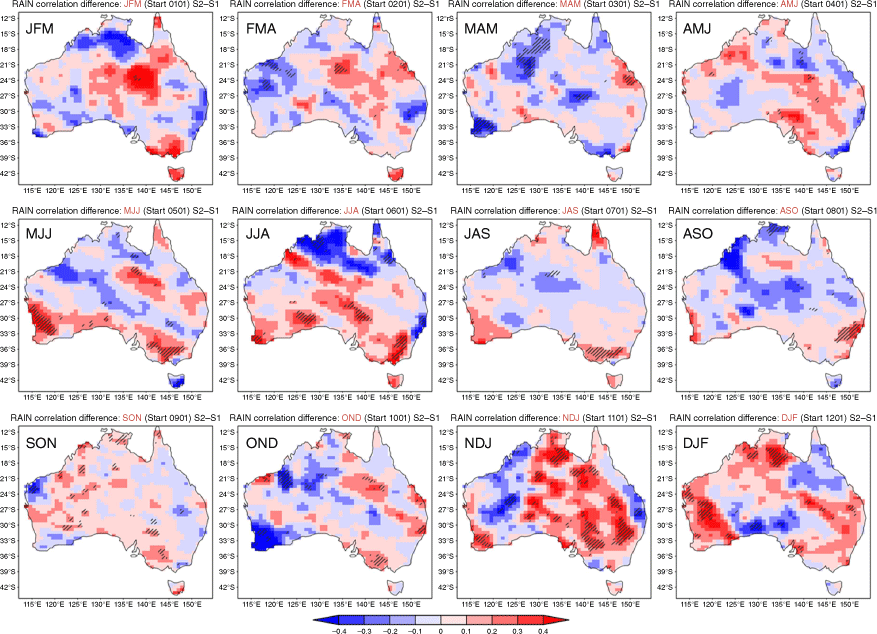
Other regional and seasonal differences in skill between ACCESS-S1 and ACCESS-S2 are patchy and require additional analysis to determine which are true signals or are noise, and to then attribute the change in skill to differences between the two systems. For example, Fig. 24 shows the difference in correlation skill for forecasts of seasonal mean rainfall for the first season of the forecast (red indicates ACCESS-S2 is more skilful than ACCESS-S1). The results are mixed, although the large signals are generally in favour of ACCESS-2 being an improvement over ACCESS-S1. Some of the large signals in the dry season should be ignored (e.g. over northern Australia in winter, JJA), since there is virtually no rainfall at that time. The increase in skill over southern Australia for May–June–July (MJJ) may be due to soil moisture initialisation, based on previous sensitivity experiments on the impact of soil moisture initialisation (Zhao et al. 2017). The 23-year common hindcast period between ACCESS-S1 and ACCESS-S2 is small for detecting significant changes in forecast performance on regional scales, especially for a highly variable quantity like rainfall. As mentioned previously, additional sensitivity studies are required to delve deeper into any differences in skill and will be part of future papers.
The difference in correlation skill for 0-month lead time seasonal rainfall anomalies (i.e. S0, as defined in Fig. 21) between ACCESS-S2 and ACCESS-S1, initialised on the 1st of each month for the period 1990–2012 and based on 21/22-member time-lagged ensembles (as described in Fig. 21). Verification data are the Australian Water Availability Project (AWAP) gridded datasets (Jones et al. 2009). Red colours indicate higher correlations in ACCESS-S2. The hatched lines represent the significant correlation differences, determined by bootstrapping (as described for Fig. 22). JFM, January–February–March; FMA, February–March–April, etc.
5. Summary and conclusions
This paper describes the ACCESS-S2 seasonal prediction system, which became operational at the Bureau of Meteorology in October 2021, replacing ACCESS-S1.
Significant changes with this upgrade include:
A new weakly coupled ensemble optimum-interpolation DA scheme, which produces initial conditions for the ocean, atmosphere, sea-ice and land surface (including realistic time-varying soil moisture);
Earlier delivery of multi-week forecasts to meet customers’ needs, due to more timely initial conditions provided by the new DA system;
Improved operational resilience by removing the dependency on the provision of Met Office ocean and sea ice initial conditions;
A longer hindcast set (38 compared to 23 years) with a modified ensemble design which is beneficial for forecast calibration, estimates of skill of the system and inclusion of additional cases of low-frequency climate drivers;
Enhanced post-processing. More outputs are available to users and reduced computation is required by Climate Services or users.
Analysis of the reanalysis and hindcasts provide the expectation that ACCESS-S2 will deliver improved forecast accuracy compared to ACCESS-S1. In particular, there are improvements in forecast performance over Australia related to the more realistic initialisation of soil moisture, and indications that the ocean DA has led to improvements in the ability to predict ENSO.
Key results in performance of ACCESS-S2 can be summarised as follows:
There are some issues with the ocean initial conditions used for ACCESS-S1 (Blockley et al. 2014), particularly related to the ocean currents, which are important for ENSO predictions. The ACCESS-S2 initial ocean states are improved compared to those used by ACCESS-S1.
There are improved forecasts of ENSO, particularly for forecasts started in autumn. This is an excellent result as autumn is a challenging time of year for predictions, with all seasonal prediction models experiencing some difficulty in predicting the development or decay of ENSO at that time.
One of the advances of ACCESS-S2 over ACCESS-S1 is the realistic initialisation of soil moisture. This has resulted in a clear improvement in the skill of maximum temperature forecasts over northern, eastern and western Australia in ACCESS-S2 in the first month of the forecast and in the winter half of the year.
ACCESS-S2 represents another step forward in the development of seasonal forecast systems at the Bureau of Meteorology, with advances in DA leading to key improvements in forecast performance. However, many of the known deficiencies in ACCESS-S1 remain, such as rainfall and SST biases in the Indian Ocean and Maritime Continent regions that are detrimental for teleconnections to Australian climate (Hudson et al. 2017). These persistent biases are currently the focus of a key collaboration with the Met Office and other partners, and the results will provide opportunities for future improvements in seasonal forecasting.
Data availability
ACCESS-S2 data are published on the National Computational Infrastructure (NCI) and are available for research purposes. The data collection comprises three records: (1) the initial conditions used for the hindcasts, (2) the ocean reanalysis and (3) the hindcasts, including the 5-km calibrated variables. https://geonetwork.nci.org.au/geonetwork/srv/eng/catalog.search#/metadata/f3311_4920_0252_8073.
Conflicts of interest
Eun-Pa Lim is an Associate Editor for the Journal of Southern Hemisphere Earth Systems Science but did not at any stage have editor-level access to this manuscript while in peer review, as is the standard practice when handling manuscripts submitted by an editor to this journal. The Journal of Southern Hemisphere Earth Systems Science encourages its editors to publish in the journal and they are kept totally separate from the decision-making processes for their manuscripts. The authors have no further conflicts of interest to declare.
Acknowledgements
The authors gratefully acknowledge the project leadership of Manoshan Domingo; and the NCI facility and the Bureau of Meteorology Scientific Computing Services for technical support. The authors thank Avijeet Ramchurn and Tim Cowan for reviewing the manuscript. The authors acknowledge the contribution of Angus Gray-Weale in the technical aspects of the data assimilation functionality and the generation of the reanalysis.
References
Argo (2000) Argo float data and metadata from Global Data Assembly Centre. (Argo GDAC). (SEANOE) 10.17882/42182
Ashok K, Behera SK, Rao SA, Weng H, Yamagata T (2007) El Niño Modoki and its possible teleconnection. Journal of Geophysical Research: Oceans 112, C1107.
| Crossref | Google Scholar |
Banzon V, Smith TM, Chin TM, Liu C, Hankins W (2016) A long-term record of blended satellite and in situ sea-surface temperature for climate monitoring, modeling and environmental studies. Earth System Science Data 8, 165-176.
| Crossref | Google Scholar |
Barnston AG, Tippett MK, L’Heureux ML, et al. (2012) Skill of real-time seasonal ENSO model predictions during 2002–11: is our capability increasing? Bulletin of the American Meteorological Society 93, 631-651.
| Crossref | Google Scholar |
Best MJ, Pryor M, Clark DB, et al. (2011) The Joint UK Land Environment Simulator (JULES), model description – part 1: energy and water fluxes. Geoscientific Model Development 4, 677-699.
| Crossref | Google Scholar |
Blockley EW, Martin MJ, McLaren AJ, Ryan AG, Waters J, Lea DJ, Mirouze I, Peterson KA, Sellar A, Storkey D (2014) Recent development of the Met Office operational ocean forecasting system: an overview and assessment of the new Global FOAM forecasts. Geoscientific Model Development 7, 2613-2638.
| Crossref | Google Scholar |
Bourlès B, Lumpkin R, McPhaden MJ, Hernandez F, Nobre P, Campos E, Yu L, Planton S, Busalacchi A, Moura AD, Servain J, Trotte J (2008) The PIRATA Program: history, accomplishments, and future directions. Bulletin of the American Meteorological Society 89, 1111-1126.
| Crossref | Google Scholar |
Bowler NE, Arribas A, Beare SE, Mylne KR, Shutts GJ (2009) The local ETKF and SKEB: upgrades to the MOGREPS short-range ensemble prediction system. Quarterly Journal of the Royal Meteorological Society 135(640), 767-776.
| Crossref | Google Scholar |
Brassington GB, Freeman J, Huang X, Pugh T, Oke PR, Sandery PA, Taylor A, Andreu-Burillo I, Schiller A, Griffin DA, Fiedler R, Mansbridge J, Beggs H, Spillman CM (2012) Ocean model, analysis and prediction system: version 2. CAWCR Technical Report 52. (Centre for Australian Weather and Climate Research) Available at http://www.bom.gov.au/research/publications/cawcrreports/CTR_052.pdf
Bureau of Meteorology (2019a) APS3 upgrade of the ACCESS-G/GE Numerical Weather Prediction System. (BOM) Available at http://www.bom.gov.au/australia/charts/bulletins/opsbull_G3GE3_external_v3.pdf
Bureau of Meteorology (2019b) Operational implementation of ACCESS-S1 forecast post-processing (Melbourne). (BOM) Available at http://www.bom.gov.au/australia/charts/bulletins/opsull-124-ext.pdf
Cai W, van Rensch P, Cowan T, Hendon HH (2011) Teleconnection pathways of ENSO and the IOD and the mechanisms for impacts on Australian rainfall. Journal of Climate 24, 3910-3923.
| Crossref | Google Scholar |
Collins WJ, Bellouin N, Doutriaux-Boucher M, et al. (2011) Development and evaluation of an Earth-System model – HadGEM2. Geoscientific Model Development 4, 1051-1075.
| Crossref | Google Scholar |
de Burgh-Day C, Griffiths M, Yan H, Young G, Hudson D, Alves O (2020) An adaptable framework for development and real time production of experimental sub-seasonal to seasonal forecast products. Bureau Research Report 42. (Australian Bureau of Meteorology) Available at http://www.bom.gov.au/research/research-reports.shtml
Dee DP, Uppala SM, Simmons AJ, et al. (2011) The ERA-Interim reanalysis: configuration and performance of the data assimilation system. Quarterly Journal of the Royal Meteorological Society 137, 553-597.
| Crossref | Google Scholar |
Evensen G (2003) The ensemble Kalman filter: theoretical formulation and practical implementation. Ocean Dynamics 53, 343-367.
| Crossref | Google Scholar |
Gasparin F, Cravatte S, Greiner E, Perruche C, Hamon M, Van Gennip S, Lellouche JM (2021) Excessive productivity and heat content in tropical Pacific analyses: disentangling the effects of in situ and altimetry assimilation. Ocean Modelling 160, 101768.
| Crossref | Google Scholar |
Goni G, Roemmich DE, Molinari RO, Meyers GA, Sun CH, Boyer T, Baringer MO, Gouretski VI, Di Nezio PE, Reseghetti FR, Vissa GO (2010) The ship of opportunity program. In ‘Proceedings of OceanObs ‘09: Sustained Ocean Observations and Information for Society (Vol. 2)’, 21–25 September 2009, Venice, Italy. (Eds J Hall, DE Harrison, D Stammer) ESA Publication WPP-306. (European Space Agency) 10.5270/OceanObs09.cwp.35
Good SA, Martin MJ, Rayner NA (2013) EN4: Quality controlled ocean temperature and salinity profiles and monthly objective analyses with uncertainty estimates. Journal of Geophysical Research: Oceans 118(12), 6704-6716.
| Crossref | Google Scholar |
Gouretski V, Reseghetti F (2010) On depth and temperature biases in bathythermograph data: development of a new correction scheme based on analysis of a global ocean database. Deep Sea Research – I. Oceanographic Research Papers 57, 812-833.
| Crossref | Google Scholar |
Hayes SP, Mangum LJ, PiCaut J, Sumi A, Takeuchi K (1991) TOGA-TAO: a moored array for real-time measurements in the tropical Pacific Ocean. Bulletin of the American Meteorological Society 72, 339-347.
| Crossref | Google Scholar |
Hendon HH, Thompson DWJ, Wheeler MC (2007) Australian rainfall and surface temperature variations associated with the Southern Hemisphere Annular Mode. Journal of Climate 20, 2452-2467.
| Crossref | Google Scholar |
Hendon HH, Lim E, Wang G, Alves O, Hudson D (2009) Prospects for predicting two flavors of El Niño. Geophysical Research Letters 36(19), L19713.
| Crossref | Google Scholar |
Hendon HH, Lim E-P, Abhik S (2020) Impact of interannual ozone variations on the downward coupling of the 2002 Southern Hemisphere Stratospheric Warming. Journal of Geophysical Research: Atmospheres 125, e2020JD032952.
| Crossref | Google Scholar |
Huang B, Liu C, Banzon V, Freeman E, Graham G, Hankins B, Smith T, Zhang H-M (2021) Improvements of the Daily Optimum Interpolation Sea Surface Temperature (DOISST) version 2.1. Journal of Climate 34, 2923-2939.
| Crossref | Google Scholar |
Hudson D, Alves O, Hendon HH, Lim E-P, Liu G, Luo J-J, MacLachlan C, Marshall AG, Shi L, Wang G, Wedd R, Young G, Zhao M, Zhou X (2017) ACCESS-S1: The new Bureau of Meteorology multi-week to seasonal prediction system. Journal of Southern Hemisphere Earth Systems Science 67(3), 132-159.
| Crossref | Google Scholar |
Jones DA, Wang W, Fawcett R (2009) High-quality spatial climate data-sets for Australia. Australian Meteorological and Oceanographic Journal 58, 233-248.
| Crossref | Google Scholar |
Kalnay E, Kanamitsu M, Kistler R, et al. (1996) The NCEP/NCAR 40-year reanalysis project. Bulletin of the American Meteorological Society 77, 437-471.
| Crossref | Google Scholar |
Kobayashi S, Ota Y, Harada Y, Ebita A, Moriya M, Onoda H, Onogi K, Kamahori H, Kobayashi C, Endo H, Miyaoka K, Takahashi K (2015) The JRA-55 reanalysis: general specifications and basic characteristics. Journal of the Meteorological Society of Japan, Series II 93(1), 5-48.
| Crossref | Google Scholar |
Lim E-P, Hendon HH (2015a) Understanding the contrast of Australian springtime rainfall of 1997 and 2002 in the frame of two flavors of El Niño. Journal of Climate 28, 2804-2822.
| Crossref | Google Scholar |
Lim E-P, Hendon HH (2015b) Understanding and predicting the strong Southern Annular Mode and its impact on the record wet east Australian spring 2010. Climate Dynamics 44, 2807-2824.
| Crossref | Google Scholar |
Lim E-P, Hendon HH, Arblaster JM, Chung C, Moise AF, Hope P, Young G, Zhao M (2016) Interaction of the recent 50 year SST trend and La Niña 2010: amplification of the Southern Annular Mode and Australian springtime rainfall. Climate Dynamics 47(7–8), 2273-2291.
| Crossref | Google Scholar |
Lim Y, Son S-W, Kim D (2018) MJO prediction skill of the subseasonal-to-seasonal prediction models. Journal of Climate 31, 4075-4094.
| Crossref | Google Scholar |
Lim E-P, Hendon HH, Boschat G, Hudson D, Thompson DWJ, Dowdy AJ, Arblaster JM (2019) Australian hot and dry extremes induced by weakenings of the stratospheric polar vortex. Nature Geoscience 12, 896-901.
| Crossref | Google Scholar |
Lim E-P, Hendon HH, Shi L, de Burgh-Day C, Hudson D, King A, Trewin B, Griffiths M, Marshall A (2021a) Tropical forcing of Australian extreme low minimum temperatures in September 2019. Climate Dynamics 56, 3625-3641.
| Crossref | Google Scholar |
Lim E-P, Hendon HH, Butler AH, et al. (2021b) The 2019 southern hemisphere polar stratospheric warming and its impacts. Bulletin of the American Meteorological Society 102, E1150-E1171.
| Crossref | Google Scholar |
Locarnini RA, Mishonov AV, Baranova OK, Boyer TP, Zweng MM, Garcia HE, Reagan JR, Seidov D, Weathers K, Paver CR, Smolyar I (2018) World Ocean Atlas 2018, Volume 1: Temperature. NOAA Atlas NESDIS 81. (Ed. A Mishonov) (US Department of Commerce, National Oceanic and Atmospheric Administration: Silver Spring, MD, USA) Available at https://www.ncei.noaa.gov/sites/default/files/2020-04/woa18_vol1.pdf
MacLachlan C, Arribas A, Peterson KA, Maidens A, Fereday D, Scaife AA, Gordon M, Vellinga M, Williams A, Comer RE, Camp J, Xavier P, Madec G (2015) Global Seasonal forecast system version 5 (GloSea5): a high-resolution seasonal forecast system. Quarterly Journal of the Royal Meteorological Society 141, 1072-1084.
| Crossref | Google Scholar |
Madec G, Bourdallé-Badie R, Bouttier P-A, Bricaud C, Bruciaferri D, Calvert D, Chanut J, Clementi E, Coward A, Delrosso D, Ethé C, Flavoni S, Graham T, Harle J, Iovino D, Lea D, Lévy C, Lovato T, Martin M, Masson S, Mocavero S, Paul J, Rousset C, Storkey D, Storto A, Vancoppenolle M (2013) NEMO ocean engine. Notes du Pôle de modélisation de l'Institut Pierre-Simon Laplace 27, v3.4-patch.
| Crossref | Google Scholar |
Madec G, Bourdallé-Badie R, Chanut J, Clementi E, Coward A, Ethé C, Iovino D, Lea D, Lévy C, Lovato T, Martin N, Masson S, Mocavero S, Rousset C, Storkey D, Müeller S, Nurser G, Bell M, Samson G, Mathiot P, Mele F, Moulin A (2022) NEMO ocean engine. Scientific Notes of IPSL Climate Modelling Center 27, 4.2.
| Crossref | Google Scholar |
Maharaj EA, Wheeler MC (2005) Forecasting an index of the Madden-oscillation. International Journal of Climatology 25, 1611-1618.
| Crossref | Google Scholar |
Marshall AG, Hudson D, Wheeler MC, Hendon HH, Alves O (2011) Assessing the simulation and prediction of rainfall associated with the MJO in the POAMA seasonal forecast system. Climate Dynamics 37, 2129-2141.
| Crossref | Google Scholar |
Marshall AG, Hudson D, Wheeler MC, Hendon HH, Alves O (2012) Simulation and prediction of the Southern Annular Mode and its influence on Australian intra-seasonal climate in POAMA. Climate Dynamics 38, 2483-2502.
| Crossref | Google Scholar |
Marshall AG, Hudson D, Wheeler MC, Alves O, Hendon HH, Pook MJ, Risbey JS (2014) Intra-seasonal drivers of extreme heat over Australia in observations and POAMA-2. Climate Dynamics 43, 1915-1937.
| Crossref | Google Scholar |
Marshall AG, Hendon HH, Hudson D (2021) Influence of the Madden–Julian Oscillation on multiweek prediction of australian rainfall extremes using the ACCESS-S1 prediction system. Journal of Southern Hemisphere Earth Systems Science 71, 159-180.
| Crossref | Google Scholar |
Marshall AG, Gregory PA, de Burgh-Day CO, Griffiths M (2022) Subseasonal drivers of extreme fire weather in Australia and its prediction in ACCESS-S1 during spring and summer. Climate Dynamics 58, 523-553.
| Crossref | Google Scholar |
McPhaden MJ, Meyers G, Ando K, Masumoto Y, Murty VSN, Ravichandran M, Syamsudin F, Vialard J, Yu L, Yu W (2009) RAMA: the research moored array for African–Asian–Australian monsoon analysis and prediction. Bulletin of the American Meteorological Society 90, 459-480.
| Crossref | Google Scholar |
Megann A, Storkey D, Aksenov Y, Alderson S, Calvert D, Graham T, Hyder P, Siddorn J, Sinha B (2014) GO5.0: the joint NERC–Met Office NEMO global ocean model for use in coupled and forced applications. Geoscientific Model Development 7, 1069-1092.
| Crossref | Google Scholar |
Mirouze I, Weaver AT (2010) Representation of correlation functions in variational assimilation using an implicit diffusion operator. Quarterly Journal of the Royal Meteorological Society 136, 1421-1443.
| Crossref | Google Scholar |
Oke PR, Brassington GB, Griffin DA, Schiller A (2008) The Bluelink ocean data assimilation system (BODAS). Ocean Modelling 21, 46-70.
| Crossref | Google Scholar |
Park JY, Stock C A, Yang X, Dunne JP, Rosati A, John J, Zhang S (2018) Modeling global ocean biogeochemistry with physical data assimilation: a pragmatic solution to the equatorial instability. Journal of Advances in Modeling Earth Systems 10, 891-906.
| Crossref | Google Scholar |
Rae JGL, Hewitt HT, Keen AB, Ridley JK, West AE, Harris CM, Hunke EC, Walters DN (2015) Development of the Global Sea Ice 6.0 CICE configuration for the Met Office Global Coupled Model. Geoscientific Model Development 8, 2221-2230.
| Crossref | Google Scholar |
Reynolds RW, Rayner NA, Smith TM, Stokes DC, Wang W (2002) An improved in situ and satellite SST analysis for climate. Journal of Climate 15, 1609-1625.
| Crossref | Google Scholar |
Reynolds RW, Smith TM, Liu C, et al. (2007) Daily high-resolution-blended analyses for sea surface temperature. Journal of Climate 20, 5473-5496.
| Crossref | Google Scholar |
Risbey JS, Pook MJ, McIntosh PC, Wheeler MC, Hendon HH (2009) On the remote drivers of rainfall variability in Australia. Monthly Weather Review 137, 3233-3253.
| Crossref | Google Scholar |
Saji NH, Goswami BN, Vinayachandran PN, Yamagata T (1999) A dipole mode in the tropical Indian Ocean. Nature 401, 360-363.
| Crossref | Google Scholar |
Sakov P (2014) EnKF-C user guide. arXiv: Computer Science 1410.1233, v1. 10.48550/arXiv.1410.1233
Sakov P, Sandery P (2017) An adaptive quality control procedure for data assimilation. Tellus A 69(1), 1318031.
| Crossref | Google Scholar |
Valcke S (2013) The OASIS3 coupler: a European climate modelling community software. Geoscientific Model Development 6, 373-388.
| Crossref | Google Scholar |
Walters D, Boutle I, Brooks M, et al. (2017) The Met Office Unified Model Global Atmosphere 6.0/6.1 and JULES Global Land 6.0/6.1 configurations. Geoscientific Model Development 10, 1487-1520.
| Crossref | Google Scholar |
Wang G, Hendon HH (2007) Sensitivity of Australian rainfall to inter-El Niño variations. Journal of Climate 20, 4211-4226.
| Crossref | Google Scholar |
Wang G, Hendon HH (2020) Impacts of the Madden–Julian Oscillation on wintertime Australian minimum temperatures and Southern Hemisphere circulation. Climate Dynamics 55, 3087-3099.
| Crossref | Google Scholar |
Waters J, Lea DJ, Martin MJ, et al. (2015) Implementing a variational data assimilation system in an operational 1/4 degree global ocean model. Quarterly Journal of the Royal Meteorological Society 141, 333-349.
| Crossref | Google Scholar |
Waters J, Bell MJ, Martin MJ, Lea DJ (2017) Reducing ocean model imbalances in the equatorial region caused by data assimilation. Quarterly Journal of the Royal Meteorological Society 143, 195-208.
| Crossref | Google Scholar |
Weaver AT, Deltel C, Machu E, Ricci S, Daget N (2005) A multivariate balance operator for variational ocean data assimilation. Quarterly Journal of the Royal Meteorological Society 131, 3605-3625.
| Crossref | Google Scholar |
Webster PJ (1995) The annual cycle and the predictability of the tropical coupled ocean-atmosphere system. Meteorology and Atmospheric Physics 56(1), 33-55.
| Crossref | Google Scholar |
Wedd R, Stringer M, Haines K (2015) Argo real-time quality control intercomparison. Journal of Operational Oceanography 8(2), 108-122.
| Crossref | Google Scholar |
Wheeler MC, Hendon HH (2004) An all-season real-time multivariate MJO Index: development of an index for monitoring and prediction. Monthly Weather Review 132(8), 1917-1932.
| Crossref | Google Scholar |
Wheeler MC, Hendon HH, Cleland S, Meinke H, Donald A (2009) Impacts of the Madden–Julian Oscillation on Australian rainfall and circulation. Journal of Climate 22, 1482-1498.
| Crossref | Google Scholar |
White CJ, Hudson D, Alves O (2014) ENSO, the IOD and the intraseasonal prediction of heat extremes across Australia using POAMA-2. Climate Dynamics 43(7-8), 1791-1810.
| Crossref | Google Scholar |
Wilk MB, Gnanadesikan R (1968) Probability plotting methods for the analysis of data. Biometrika 55(1), 1-17.
| Crossref | Google Scholar |
Williams KD, Harris CM, Bodas-Salcedo A, et al. (2015) The Met Office Global Coupled model 2.0 (GC2) configuration. Geoscientific Model Development 8, 1509-1524.
| Crossref | Google Scholar |
Yin Y, Alves O, Oke PR (2011) An ensemble ocean data assimilation system for seasonal prediction. Monthly Weather Review 139, 786-808.
| Crossref | Google Scholar |
Zhao M, Zhang H-Q, Dharssi I (2017) Impact of land–surface initialization on ACCESS-S1 and comparison with POAMA. Bureau Research Report 23. (Australian Bureau of Meteorology) Available at http://www.bom.gov.au/research/research-reports.shtml
Zhong A, Beggs H (2008) Operational implementation of global australian multi-sensor sea surface temperature analysis. Analysis and prediction. Operations Bulletin 77. (Australian Bureau of Meteorology: Melbourne, Vic., Australia) Available at http://www.bom.gov.au/australia/charts/bulletins/apob77.pdf
Zweng MM, Reagan JR, Antonov JI, Locarnini RA, Mishonov AV, Boyer TP, Garcia HE, Baranova OK, Johnson DR, Seidov D, Biddle MM (2013) World Ocean Atlas 2013. Volume 2: Salinity. NOAA Atlas NESDIS 74. (Eds S Levitus, A Mishonov) (US Department of Commerce, National Oceanic and Atmospheric Administration: Silver Spring, MD, USA) Available at https://repository.library.noaa.gov/view/noaa/14848

