

Visualising Fe speciation diversity in ocean particulate samples by micro X-ray absorption near-edge spectroscopy
Matthew A. Marcus A C and Phoebe J. Lam BA Advanced Light Source, Lawrence Berkeley National Laboratory, Berkeley, CA 94720, USA.
B Department of Marine Chemistry and Geochemistry, Woods Hole Oceanographic Institution, Woods Hole, MA 02543, USA.
C Corresponding author. Email: mamarcus@lbl.gov
Environmental Chemistry 11(1) 10-17 https://doi.org/10.1071/EN13075
Submitted: 4 April 2013 Accepted: 1 August 2013 Published: 9 October 2013
Environmental context. Iron-bearing particles in the ocean have attracted interest due to the role of iron as an essential nutrient for microscopic algae, which form the base of the marine food chain. Modern techniques make it possible to analyse individual particles of iron to determine their composition, but the resulting flood of data can be overwhelming. We show a method of simplifying the data to answer such questions as what groups of minerals are present and whether they are different between ocean basins.
Abstract. It is a well known truism that natural materials are inhomogeneous, so analysing them on a point-by-point basis can generate a large volume of data, from which it becomes challenging to extract understanding. In this paper, we show an example in which particles taken from the ocean in two different regions (the Western Subarctic Pacific and the Australian sector of the Southern Ocean, south of Tasmania) are studied by Fe K-edge micro X-ray absorption near-edge spectroscopy (μXANES). The resulting set of data consists of 209 spectra from the Western Subarctic Pacific and 126 from the Southern Ocean. We show the use of principal components analysis with an interactive projection visualisation tool to reduce the complexity of the data to something manageable. The Western Subarctic Pacific particles were grouped into four main populations, each of which was characterised by spectra consistent with mixtures of 1–3 minerals: (1) Fe3+ oxyhydroxides + Fe3+ clays + Fe2+ phyllosilicates, (2) Fe3+ clays, (3) mixed-valence phyllosilicates and (4) magnetite + Fe3+ clays + Fe2+ silicates, listed in order of abundance. The Southern Ocean particles break into three clusters: (1) Fe3+-bearing clays + Fe3+ oxyhydroxides, (2) Fe2+ silicates + Fe3+ oxyhydroxides and (3) Fe3+ oxides + Fe3+-bearing clays + Fe2+ silicates, in abundance order. Although there was some overlap between the two regions, this analysis shows that the particulate Fe mineral assemblage is distinct between the Western Subarctic Pacific and the Southern Ocean, with potential implications for the bioavailability of particulate Fe in these two iron-limited regions. We then discuss possible advances in the methods, including automatic methods for characterising the structure of the data.
Introduction
The well known fact that natural materials are inhomogeneous has helped drive the development of X-ray microprobe techniques for the study of environmental, oceanographic and geological samples. In particular, the micrometre scale has proven to be a fruitful realm for such studies.[1,2] Until now, the procedure for doing microprobe studies in the hard X-ray region has been to map the sample, then select a few spots of interest on which to do X-ray spectroscopy. However, such a limited number of spectra make it difficult to understand the true nature of the sample. How many minerals are present? How do samples taken from different areas differ? Are there distinct environments for the element of interest, or a continuous range of speciation within the sampled area?
Chemical species mapping is one method that allows for a quick assessment of the distribution of different chemical states of a given element in a sample. Traditionally, several X-ray maps (typically n ≤ 5) are taken of the same area at energies close to an absorption edge of that element. The shape and position in energy of the edge depend on the chemical state of the element, so performing maps at a set of well chosen energies yields spatially resolved chemical speciation information, for instance the distribution of Fe2+ v. Fe3+.[3–5] Essentially, one gets a tabulated micro-XANES (X-ray absorption near-edge structure) spectrum at each pixel. Although chemical mapping is a quick and efficient way of surveying the spatial distribution of speciation for a given element, it has disadvantages because the maps are typically done at a small number of energies, so the information at each pixel corresponds to a XANES ‘spectrum’ taken at only a few points. Suppose one is looking for the distributions of Fe2+ and Fe3+. The use of traditional valence-state mapping is tantamount to the assumption that the absorption spectra for all Fe2+ species look alike and likewise for Fe3+, which is not so. If one knows which species are present in the sample by other means, then the errors resulting from this faulty assumption may be avoided, but we often don't have this information. Nowadays, due to technical advances in hard X-ray microprobes such as the Maia detector[6] and undulator sources, it is becoming practical to take full XANES spectra at many different spots, thus allowing an approach to statistical sampling in addition to characterisation of specific features at the micrometre scale. In the soft X-ray arena, ‘stacks’ consisting of maps taken at many energies are routinely collected. Each pixel of such a stack represents a μXANES spectrum for that pixel.[7]
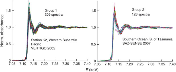
Even if one doesn't take a spectrum at each pixel, it is still quite possible to wind up with many more spectra than can be understood by visual inspection or least-squares fitting of each one. In this paper, we show such an example. Fe-bearing marine suspended particles were filtered from the ocean at two different locations, and the filters mapped by micro X-ray fluorescence (μXRF). Fe K-edge μXANES spectra were taken on 209 particles from one site and 126 from the other. Fig. 1 shows these spectra. No obvious conclusions can be drawn simply by looking at the two sets of curves. Linear-combination fitting, with all its ambiguities, is also not likely to be helpful if blindly applied to all 335 spectra using a large database of standards. Although few studies generate such numbers of spectra now, it is clear that the new hardware becoming available will make this circumstance more common in the future.
|
The reason we took all those spectra is, of course, to gain scientific insight about the forms of particulate Fe in the ocean. Characterisation of the chemical form of marine particulate iron helps to address two major uncertainties in the biogeochemical cycling of iron in the ocean: the sources of iron to the ocean and the bioavailability of different sources of iron.
Studies using chemical species mapping techniques and soft X-ray spectroscopy are already starting to demonstrate the chemical and geographic diversity of particulate Fe in some parts of the ocean.[3,8] Fe K-edge µ-XANES can provide even more detailed chemical information that will deepen our understanding of iron cycling in the ocean, provided we have the tools that will help us collect and analyse this data effectively. Specifically, we would like to know:
-
Can we explain the data in terms of a small number of types of material?
-
How many different types of spectra are there?
-
In what way are the two sampling locations different?
In this paper, we use the example cited above to demonstrate an approach to simplifying the dataset so that the salient features become comprehensible. As has become standard in the soft X-ray range,[9] we decompose the dataset using principal components analysis (PCA) and represent each spectrum as a point in a multi-dimensional vector space, such that the first few components are the most significant. We then ignore the higher (minor) components and search for clusters. In previous papers such as Lerotic et al.,[9] the points were plotted in coordinates corresponding to the loadings for specified components, so, for instance, the x-axis might be the second component and the y-axis the third. We extend this idea by applying an interactive tool that lets the user rotate the cloud of points around chosen axes, thus making visible separations between clusters of points that don't show up in the Cartesian-axes plots. By viewing the points as one rotates them, one gets an impression of three-dimensional structure.
Methods
Size-fractionated suspended marine particulate samples were collected between the surface and 1000 m by in-situ filtration on a 51-µm polyester prefilter followed by quartz fibre filters (nominal 1-µm pore size). All filters were acid leached before use. The Western Subarctic Pacific samples were collected in July–August 2005 in the Western Subarctic Pacific during the VERTIGO (Vertical Transport in the Global Ocean) project at Station K2 (47°N, 161°W).[10–12] Some sinking particles collected by trace-metal clean sediment traps[13] were also analysed at the beamline; these samples were filtered onto acid-leached polycarbonate membrane filters. Southern Ocean samples were collected in January–February 2007 in subtropical, subantarctic and polar frontal waters south of Tasmania during the SAZ-SENSE (Sensitivity of the Subantarctic Zone to Environmental Change) project.[14] All samples were misted with ultrapure water at sea to reduce salt and dried for 12 h at 60 °C and stored dried. Because of the sample preservation procedure employed for these samples, any unstable Fe species would have oxidised, so the Fe speciation presented here represents the stable, more crystalline mineral component of the sample.
The Western Subarctic Pacific XANES spectra were from both sediment trap (150, 300, 500 m) and 1–51-µm and >51-µm in-situ filtration samples (60–480 m) from a single station.[11,13] The Southern Ocean XANES spectra were collected on 1–51-µm in-situ filtration samples from five stations at up to six depths in the upper 800 m per station: P1 – Subantarctic-West, P2 – Polar Front, P3 – Subantarctic-East, and Stations 23 and 24 in East Australian Current (EAC)-influenced subtropical waters south-east of Tasmania.[14] For the purposes of the analysis presented here, we have grouped all spectra from samples from the Western Subarctic Pacific into ‘Group 1’ (n = 209) and all spectra from samples from the Southern Ocean into ‘Group 2’ (n = 126).
Particulate samples on their filter substrates were directly mounted at the beamline for mapping by µXRF and spectroscopy by extended µXANES. Typically, a 500 × 500-µm2 map was collected at 10 keV for each sample with an ~5-µm step size, and ~5–10 Fe-rich spots of varying intensities were chosen randomly from the Fe Kα map for spectroscopic analysis. Fe K-edge extended µXANES spectra were collected between 7010 and 7415 eV, with 0.5-eV steps through the Fe K-edge region (7095–7140 eV), and at 1, 2 and 5-eV steps at higher energies. XANES spectra were corrected for detector dead-time, had their pre-edges subtracted, and normalised using software available at the beamline.[15] Energy calibration was ensured using a reproducible glitch in the monochromator at 7263.64 eV and the spectra shifted as necessary.
Once a set of spectra such as those described above has been reduced to pre-edge-subtracted, post-edge-normalised form, the work of classification can begin. The first step is to do PCA on the set and decide how many components to retain. Separation of clusters may be possible with fewer components than is really necessary to describe the full variability of the dataset. Let the ith spectrum be denoted yi(E) with i = 1…n. Using PCA, we approximate the set of spectra as:
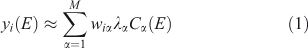
where M is the number of components retained, wiα is the amount (loading) of component α assigned to spectrum i, λα is the eigenvalue (relative importance) of component α, and Cα(E) is the αth abstract component. The eigenvalues are sorted by magnitude so that the first component is the most important. The abstract components form an orthonormal set. For XANES data with a sufficiently long post-edge region, the first abstract component approximates the average of all the spectra, and the loadings of this component for all the individual spectra are all approximately the same. We can also perform the rotation given by iterative target factor analysis (ITFA[16]), which seeks apparent end-members such that the loadings are all non-negative and as different from each other as possible, in which case we have
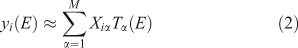
in which the loadings are Xiα and the components are Tα(E). If M is small enough, the ITFA components often look like identifiable XANES spectra.
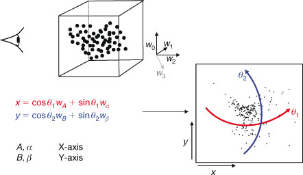
If we simply make a scatterplot of, for instance, wi2 ÷ wi1 v. wi3 ÷ wi1, as is typically done with STXM (Scanning Transmission X-ray Microscope) stacks, we often find a poor separation between sets of points representing spectra from different types of materials. By a clever choice of coordinates, we can make these separations clear, essentially using the image-processing capabilities of the human visual system. The rotation we use is chosen from a restricted set that lets one look at combinations of four weights:
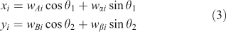
where axes A and B may be considered as ‘view’ axes, α and β are ‘hidden’ axes that are rotated into view and θ1 and θ2 are rotation angles. A schematic of how the rotation works is shown in Fig. 2. In the visualisation program, which is written in LabVIEW, the rotation angles are controlled by sliders and the axes selected by switches. The projection is shown continuously as the parameters are changed, so that the user can select rotation axes and angles that produce interesting views. As one changes θ1, there is a strong visual impression of the cloud of points as a three-dimensional object rotating around a vertical axis. Similarly, changing θ2 makes it appear as if the cloud of points is rolling around a horizontal axis. However, because the set of points exists in more than three dimensions, the choice of θ1 affects the combination of loadings that are viewed as ‘into the screen’, hence the results of changing θ2.
|
When viewing abstract components, the weights used in Eqn 3 are not quite the outputs of PCA. As mentioned above, the loading of the first component is nearly constant and a measure of intensity in the spectrum. We therefore divide other component loadings by it. This normalisation is not done for ITFA components because there's nothing special about the first one of these.
The tool has other useful features. It allows the user to select a point and see the corresponding spectrum, which is good for detecting outliers and verifying that points that are close together in projection really do correspond to similar-looking XANES spectra. It is possible to delineate clusters either by manual masking and selection or by k-means clustering.[17] The memberships of clusters thus chosen may be recorded in text files, along with the parameters used in the projection.
Results
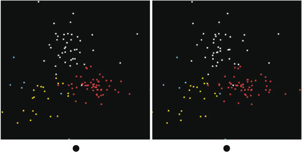
The tool described above was applied to the Western Subarctic Pacific group (Group 1), with results shown in Fig. 3. This is a stereogram obtained by taking two views with θ1 10° apart, with the points coloured according to which group (in the projected 3-D space) they belong to. Outliers are in white. The projections were done using the first six abstract PCA components. We see four distinct clusters, coloured yellow, red, cyan and purple, suggesting four distinct types of material.
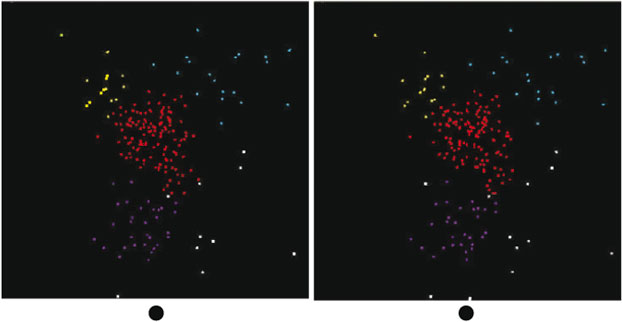
|
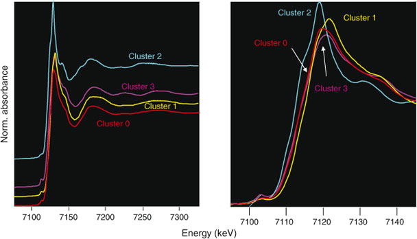
Next, we averaged the XANES spectra for each cluster, as shown in Fig. 4 and performed linear combination fitting with non-negative loadings to a large database of Fe references. This database is a revised and extended version of one used in a study of Fe XANES classification.[18] Each cluster average fit to mixtures of 1–3 minerals, as identified in Table 1. As an aside, we note that the difference between the Cluster 0 and Cluster 3 averages are subtle in the near-edge region but become more prominent in the extended region, thus showing the value of taking extended-range data even for XANES analysis.
|

|
The fits shown here for the cluster averages do not necessarily apply to the individual members. Because the cluster does take up a finite area in projection, it's obvious that the individual spectra differ from each other. Individual fits of several member of Cluster 2, for instance, always show the presence of Fe2+ phyllosilicates and Fe3+-bearing clays, but also up to 25 % of various other species such as magnetite and ferrihydrite. Thus, the fits to the cluster averages represent a simplification of the true diversity. However, the fits represent species consistently found in cluster members.
We tested the partitioning of spectra into clusters to see if this clustering really reflects diversity in the spectra. Let the normalised signal for the ith spectrun in the cth cluster be denoted yic(E) at energy point E. Define the cluster mean  where
where  represents a mean over spectra, Now define the overall mean as
  . Finally, define a diversity measure
which is, essentially, a normalised variance among the different clusters. Now, do this operation for the actual selected clusters and for ‘clusters’ made of randomly chosen spectra, such that each ‘cluster’ has the same number of spectra in it as the real ones. Spectra are chosen for ‘cluster’ membership without replacement. After 105 trials, not once did the diversity measure for the random cluster equal or exceed that for the real ones. This result suggests that the clustering organises the spectra, which differ significantly from each other, into different groups, which random allocation would not do.
Now we can ask if the Southern Ocean group (Group 2) looks the same as the Western Subarctic Pacific. One way to do this is to project the data from the Southern Ocean group onto the same basis set as the Western Subarctic Pacific group, essentially fitting the Southern Ocean group to sums of the first few abstract components found in the Western Subarctic Pacific group. By doing so, we can plot the two groups together and see if the clouds of points occupy the same space. In Fig. 5, we show a set of three rotations in which Western Subarctic Pacific points are white and Southern Ocean points are red. The red points occupy a thin slab in the projected 3-D space, whereas the white points fill the space. This shows that the Southern Ocean differs from the Western Subarctic Pacific, but does not clearly show how. We then applied the visualisation tool to the Southern Ocean group independently from the Western Subarctic Pacific group and found that it generates three clusters plus 5 % of outliers, as shown in Fig. 6, in which the outliers are the blue points. These clusters were identified using k-means clustering[17] rather than manual selection. Manual selection is an option because k-means doesn't always yield good separation. The averaged spectra from each of these clusters from the Southern Ocean are more similar to each other than those of the Western Subarctic Pacific group. One Southern Ocean cluster fits to a mix of Fe2+ silicates and Fe3+-bearing oxyhydroxides. The second cluster fits to Fe3+ clays plus oxyhydroxides and has a spectrum quite similar to that of cluster 1 in the Western Subarctic Pacific (labelled in yellow), and the third fits to hematite and smaller amounts of Fe3+ clays and Fe2+ silicates (Table 1). The exact proportions depend on which species one takes in the fits. Two of the three clusters have averages that don't fit well to sums of the cluster averages from the Western Subarctic Pacific group, which shows again that the Southern Ocean group is outside the variability of the Western Subarctic Pacific group, except possibly for outliers.

|
|
Discussion
As demonstrated above, the visualisation method is an effective way to identify clusters of similar data within a large and complex dataset so that the samples can be described in terms of a small number of types of material. Consideration of the linear combination fits of many tens to hundreds of individual spectra is an intractable problem because fits are not unique, and there is no easy way to get a sense of the overall variability in chemical speciation. The much-reduced set of variability that results from the visualisation method greatly facilitates comparisons between large datasets. In the examples presented here, the 209 spectra from the Western Subarctic Pacific were reduced to four main clusters (plus outliers), and the 126 spectra from the Southern Ocean were reduced to three main clusters (plus outliers).
Both regions contained significant amounts of Fe3+ oxyhydroxides and Fe3+-containing clays (Table 1), pointing to the ubiquity of these Fe mineral groups in marine particulate iron regardless of ocean basin. In contrast, three of the four clusters in the Western Subarctic Pacific contained Fe2+-containing phyllosilicates such as biotite or chlorite, and the fourth cluster contained significant magnetite. Neither of these mineral groups was present in the Southern Ocean clusters, indicating that these mineral groups are specific to the Western Subarctic Pacific and likely indicate the influence of the volcanic margin source of iron to that region.[3,12] Likewise, hematite was found in the Southern Ocean samples but not in the Western Subarctic Pacific. Looking more closely at the Southern Ocean group samples, we find that certain species clusters are more prevalent at some stations than others (Fig. 7). Because hematite is a known, although minor, component of mineral dust,[19] one might expect the hematite observed in our samples to derive from Australian dust. The observed higher relative abundance of the hematite-containing cluster 2 at the Polar Frontal Zone station P2 compared to the other, more northerly Subantarctic and Subtropical stations is at odds with the expected gradient from dust deposition, however, and suggests an as yet unidentified source of hematite to the Station P2 – Polar Front samples. Southern Ocean Cluster 1, which was composed entirely of Fe3+ clays and oxyhydroxides (Table 1), was the dominant species cluster at EAC-influenced subtropical stations 23 and 24. Of the three process stations, only station P3 (Subantarctic-east) was strongly influenced by this species cluster (56 % of spectra), suggesting that P3 may be the most influenced by EAC subtropical waters. Indeed, this is consistent with the conclusion derived from independent hydrographic and other trace metal data.[14] These examples show the use of Fe mineralogy as determined by µXANES analysis in tagging the source of Fe to the ocean.

|
In the example above, we found that some clusters of Fe species dominated certain stations and not others. Furthermore, there was no clear trend in species clusters with depth in the water column, supporting the idea that lateral differences in Fe speciation are generally stronger than vertical ones.
All particulate iron bioavailability studies to date have been conducted on iron oxhydroxides and iron oxides.[20,21] This XANES analysis shows that iron oxyhydroxides and oxides are only part of the particulate iron in the ocean. Journet et al.[22] and Schroth et al.[23] have both shown that Fe-containing silicates (both clays and primary minerals) from putative atmospheric dust sources can have higher solubility than iron oxides. The abundance of clays and primary and secondary Fe-bearing silicates that we see in the water column begs for the examination of the bioavailability of these particulate iron species.
Although this work was done using spectra collected on selected points, the use of fast detectors on high-flux microprobes will make it possible to collect many more spectra without the need for manual selection of points. When thousands of spectra become available on each sample, some means of visualising the structure of the data will become even more important than it is now. The present work is a start towards developing such methods.
There are several possible extensions and modifications of the basic idea of projection and dimensional reduction. For instance, instead of using model-free PCA to provide coordinates, it may be possible and sensible in some cases to do least-squares fits with non-negative coefficients on each reference spectrum. In that case, it may be necessary to add together the weights of references that are ‘similar’.
There is a class of methods called projection pursuit,[24] in which an automatic procedure is used to look for projections that are ‘interesting’ in some sense. For instance, a common criterion is that the distribution in projection should be as non-Gaussian as possible. Such an automated tool may be useful for finding combinations of coordinates not easily discovered by manual exploration.
Another class of methods starts by connecting together near-neighbour spectra into a graph (in the mathematical sense) and attempting to infer the underlying geometry of that graph. Here, ‘near-neighbour’ refers to distances between spectra computed as norms of differences between them. In spectral clustering,[25] this graph is manipulated to label each spectrum with a set of coordinates in a lower-dimensional space, much as PCA does, but without the requirement of a linear mapping between spectra and this new space. Automatic clustering methods are then used for classification, which could, in principle, be augmented with a visualisation tool such as ours. In another approach, the network of connections between spectra is fitted to the geometry of an assumed lower-dimensional manifold so that the derived points on this manifold bear the same relationship to nearby points as the corresponding spectra do to their neighbours, for example by requiring that the shortest distance between any two spectra match the geodesic distances between the corresponding points in the manifold.[26,27] Such sophisticated methods, perhaps combined with interactive visualisation tools, may be the way forward when the number of spectra goes into the hundreds or thousands.
We have demonstrated an approach to making the transition from acquiring spectra on inhomogeneous samples to acquiring a physical understanding of them. In the example shown here, we showed that data from hundreds of spectra could be simplified and some of the differences between iron-bearing particles from two parts of the ocean teased out. The combination of computation plus human visual evaluation results in a powerful tool for data analysis.
Supplementary material
An executable file of the classification program and a short ‘how-to’ guide to it are available for download from the journal, as is a copy of the Fe XANES database as used in this paper. This database does not include several species, such as Fe carbides, as they were not considered plausible possibilities for the present project.
Acknowledgements
The operations of the Advanced Light Source at Lawrence Berkeley National Laboratory are supported by the Director, Office of Science, Office of Basic Energy Sciences, US Department of Energy under contract number DE-AC02-05CH11231. Collection of samples for the VERTIGO project was supported by the US National Science Foundation Program in Chemical Oceanography to Ken Buesseler and the US Department of Energy, Office of Science, Biological and Environmental Research Program to Jim Bishop. The SAZ-SENSE project was supported by the Australian Government Cooperative Research Centres Programme. Collection of spectroscopic data by PJL was supported through the WHOI Postdoctoral Scholar Program, WHOI Independent Study Award and NSF Chemical Oceanography. Thanks to S. Fakra, S. Bone and D. Ohnemus for assistance at the beamline. The authors thank Thomas Borch, Jakob Frommer and Andreas Voegelin for the use of several of their Fe reference spectra, as well as those sources acknowledged in Marcus et al.[18]
References
[1] A. Manceau, N. Tamura, M. A. Marcus, A. A. MacDowell, R. S. Celestre, R. E. Sublett, G. Sposito, H. A. Padmore, Deciphering Ni sequestration in soil ferromanganese nodules by combining X-ray fluorescence, absorption and diffraction at micrometer scales of resolution. Am. Mineral. 2002, 87, 1494.| 1:CAS:528:DC%2BD38XotVGntb4%3D&md5=301eeefb800c1ed24c04849fb89c879fCAS |
[2] A. Manceau, M. A. Marcus, N. Tamura, Quantitative speciation of heavy metals in soils and sediments by synchrotron X-ray techniques, in Applications of Synchrotron Radiation in Low-Temperature Geochemistry and Environmental Science (Eds P. A. Fenter, M. L. Rivers, N. C. Sturchio, S. R. Sutton) 2002, pp. 341–428 (Mineralogical Society of America: Washington, DC).
[3] P. J. Lam, D. C. Ohnemus, M. A. Marcus, The speciation of marine particulate iron adjacent to active and passive continental margins. Geochim. Cosmochim. Acta 2012, 80, 108.
| The speciation of marine particulate iron adjacent to active and passive continental margins.Crossref | GoogleScholarGoogle Scholar | 1:CAS:528:DC%2BC38Xhsleqtb8%3D&md5=40ad33a1aff8b67e7bc40f3f43e55e5dCAS |
[4] I. J. Pickering, L. Gumaelius, H. H. Harris, R. C. Prince, G. Hirsch, J. A. Banks, D. E. Salt, G. N. George, Localizing the biochemical transformations of arsenate in a hyperaccumulating fern. Environ. Sci. Technol. 2006, 40, 5010.
| Localizing the biochemical transformations of arsenate in a hyperaccumulating fern.Crossref | GoogleScholarGoogle Scholar | 1:CAS:528:DC%2BD28Xms12jsLs%3D&md5=3f54a9096b27e631cd49c285007b55b2CAS | 16955900PubMed |
[5] M. A. Marcus, X-Ray photon-in/photon-out methods for chemical imaging. Trends Analyt. Chem. 2010, 29, 508.
| X-Ray photon-in/photon-out methods for chemical imaging.Crossref | GoogleScholarGoogle Scholar | 1:CAS:528:DC%2BC3cXmsVOms7Y%3D&md5=359f39f7bb949d42efd7a3bf6ac5382cCAS |
[6] B. Etschmann, C. G. Ryan, J. Brugger, R. Kirkham, R. Hough, G. Moorhead, D. Siddons, G. De Geronimo, A. Kuczewski, P. Dunn, Reduced As components in highly oxidized environments: evidence from full spectral XANES imaging using the MAIA massively parallel detector. Am. Mineral. 2010, 95, 884.
| Reduced As components in highly oxidized environments: evidence from full spectral XANES imaging using the MAIA massively parallel detector.Crossref | GoogleScholarGoogle Scholar | 1:CAS:528:DC%2BC3cXmslKksLg%3D&md5=bf4f5a2ee6fec8075e04e50390a4788dCAS |
[7] J. Lawrence, G. Swerhone, G. Leppard, T. Araki, X. Zhang, M. West, A. Hitchcock, Scanning transmission X-ray, laser scanning, and transmission electron microscopy mapping of the exopolymeric matrix of microbial biofilms. Appl. Environ. Microbiol. 2003, 69, 5543.
| Scanning transmission X-ray, laser scanning, and transmission electron microscopy mapping of the exopolymeric matrix of microbial biofilms.Crossref | GoogleScholarGoogle Scholar | 1:CAS:528:DC%2BD3sXntlSis74%3D&md5=69c9da5c7411c7ef8f7766fc71e7f2f3CAS | 12957944PubMed |
[8] B. P. von der Heyden, A. N. Roychoudhury, T. N. Mtshali, T. Tyliszczak, S. C. B. Myneni, Chemically and geographically distinct solid-phase iron pools in the Southern Ocean. Science 2012, 338, 1199.
| Chemically and geographically distinct solid-phase iron pools in the Southern Ocean.Crossref | GoogleScholarGoogle Scholar | 1:CAS:528:DC%2BC38Xhslans7nI&md5=bc2444817580dcc3d20f03b70a58ae41CAS | 23197531PubMed |
[9] M. Lerotic, C. Jacobsen, T. Schäfer, S. Vogt, Cluster analysis of soft X-ray spectromicroscopy data. Ultramicroscopy 2004, 100, 35.
| Cluster analysis of soft X-ray spectromicroscopy data.Crossref | GoogleScholarGoogle Scholar | 1:CAS:528:DC%2BD2cXltF2lsr4%3D&md5=d6c21ec6ef4fdd4b4fd0d969d66510dcCAS | 15219691PubMed |
[10] K. O. Buesseler, T. W. Trull, D. K. Steinberg, M. W. Silver, D. A. Siegel, S. Saitoh, C. H. Lamborg, P. J. Lam, D. M. Karl, N. Z. Jiao, M. C. Honda, M. Elskens, F. Dehairs, S. L. Brown, P. W. Boyd, J. K. B. Bishop, R. R. Bidigare, VERTIGO (vertical transport in the global ocean): a study of particle sources and flux attenuation in the North Pacific. Deep Sea Res. Part II Top. Stud. Oceanogr. 2008, 55, 1522.
| VERTIGO (vertical transport in the global ocean): a study of particle sources and flux attenuation in the North Pacific.Crossref | GoogleScholarGoogle Scholar |
[11] J. K. B. Bishop, T. J. Wood, Particulate matter chemistry and dynamics in the twilight zone at VERTIGO ALOHA and K2 sites. Deep Sea Res. Part I Oceanogr. Res. Pap. 2008, 55, 1684.
| Particulate matter chemistry and dynamics in the twilight zone at VERTIGO ALOHA and K2 sites.Crossref | GoogleScholarGoogle Scholar |
[12] P. J. Lam, J. K. B. Bishop, The continental margin is a key source of iron to the HNLC North Pacific ocean. Geophys. Res. Lett. 2008, 35, L07608.
| The continental margin is a key source of iron to the HNLC North Pacific ocean.Crossref | GoogleScholarGoogle Scholar |
[13] C. H. Lamborg, K. O. Buesseler, P. J. Lam, Sinking fluxes of minor and trace elements in the North Pacific ocean measured during the VERTIGO program. Deep Sea Res. Part II Top. Stud. Oceanogr. 2008, 55, 1564.
| Sinking fluxes of minor and trace elements in the North Pacific ocean measured during the VERTIGO program.Crossref | GoogleScholarGoogle Scholar |
[14] A. R. Bowie, D. Lannuzel, T. A. Remenyi, T. Wagener, P. J. Lam, P. W. Boyd, C. Guieu, A. T. Townsend, T. W. Trull, Biogeochemical iron budgets of the Southern Ocean south of Australia: decoupling of iron and nutrient cycles in the subantarctic zone by the summertime supply. Global Biogeochem. Cycles 2009, 23, GB4034.
| Biogeochemical iron budgets of the Southern Ocean south of Australia: decoupling of iron and nutrient cycles in the subantarctic zone by the summertime supply.Crossref | GoogleScholarGoogle Scholar |
[15] M. A. Marcus, A. A. MacDowell, R. Celestre, A. Manceau, T. Miller, H. A. Padmore, R. E. Sublett, Beamline 10.3.2 at ALS: a hard X-ray microprobe for environmental and materials sciences. J. Synchrotron Radiat. 2004, 11, 239.
| Beamline 10.3.2 at ALS: a hard X-ray microprobe for environmental and materials sciences.Crossref | GoogleScholarGoogle Scholar | 1:CAS:528:DC%2BD2cXjtl2gur4%3D&md5=e2476a4e81e4beb26c6ded3d8dcb11bfCAS | 15103110PubMed |
[16] A. Roßberg, T. Reich, G. Bernhard, Complexation of uranium(VI) with protocatechuic acid – application of iterative transformation factor analysis to EXAFS spectroscopy. Anal. Bioanal. Chem. 2003, 376, 631.
| Complexation of uranium(VI) with protocatechuic acid – application of iterative transformation factor analysis to EXAFS spectroscopy.Crossref | GoogleScholarGoogle Scholar | 12811445PubMed |
[17] J. Macqueen (Ed.) Some methods for classification and analysis of multivariate observations, in Proceedings of the fifth Berkeley Symposium on Mathematical Statistics and Probability, 21 June–18 July 1965, Berkeley, CA 1967, pp. 281–297 (UC Berkeley Press: Berkeley, CA; and Cambridge University Press: London).
[18] M. A. Marcus, A. J. Westphal, S. C. Fakra, Classification of Fe-bearing species from k-edge XANES data using two-parameter correlation plots. J. Synchrotron Radiat. 2008, 15, 463.
| Classification of Fe-bearing species from k-edge XANES data using two-parameter correlation plots.Crossref | GoogleScholarGoogle Scholar | 1:CAS:528:DC%2BD1cXhtVens77M&md5=72e58df6c92c0ac341ff62541fa30ff2CAS | 18728317PubMed |
[19] C. D. Koven, I. Fung, Identifying global dust source areas using high-resolution land surface form. J. Geophys. Res. – Atmos. 2008, 113, D22204.
| Identifying global dust source areas using high-resolution land surface form.Crossref | GoogleScholarGoogle Scholar |
[20] M. L. Wells, L. M. Mayer, R. R. L. Guillard, A chemical method for estimating the availability of iron to phytoplankton in seawater. Mar. Chem. 1991, 33, 23.
| A chemical method for estimating the availability of iron to phytoplankton in seawater.Crossref | GoogleScholarGoogle Scholar | 1:CAS:528:DyaK3MXktVOnu74%3D&md5=0233fd5d4048a030e5f847ea5bd59dbcCAS |
[21] H. W. Rich, F. M. M. Morel, Availability of well-defined iron colloids to the marine diatom Thalassiosira weissflogii. Limnol. Oceanogr. 1990, 35, 652.
| Availability of well-defined iron colloids to the marine diatom Thalassiosira weissflogii.Crossref | GoogleScholarGoogle Scholar | 1:CAS:528:DyaK3cXlvVOks70%3D&md5=a343829554b548e3a49aad0aae14a8fdCAS |
[22] E. Journet, K. V. Desboeufs, S. Caquineau, J. L. Colin, Mineralogy as a critical factor of dust iron solubility. Geophys. Res. Lett. 2008, 35, L07805.
| Mineralogy as a critical factor of dust iron solubility.Crossref | GoogleScholarGoogle Scholar |
[23] A. W. Schroth, J. Crusius, E. R. Sholkovitz, B. C. Bostick, Iron solubility driven by speciation in dust sources to the ocean. Nat. Geosci. 2009, 2, 337.
| Iron solubility driven by speciation in dust sources to the ocean.Crossref | GoogleScholarGoogle Scholar | 1:CAS:528:DC%2BD1MXlt1SntLo%3D&md5=f5b59601121bc7b1fe1ec90c045e4169CAS |
[24] P. J. Huber, Projection pursuit. Ann. Stat. 1985, 13, 435.
| Projection pursuit.Crossref | GoogleScholarGoogle Scholar |
[25] C. H. Yoon, P. Schwander, C. Abergel, I. Andersson, J. Andreasson, A. Aquila, S. Bajt, M. Barthelmess, A. Barty, M. J. Bogan, Unsupervised classification of single-particle X-ray diffraction snapshots by spectral clustering. Opt. Express 2011, 19, 16 542.
| Unsupervised classification of single-particle X-ray diffraction snapshots by spectral clustering.Crossref | GoogleScholarGoogle Scholar |
[26] J. B. Tenenbaum, V. De Silva, J. C. Langford, A global geometric framework for nonlinear dimensionality reduction. Science 2000, 290, 2319.
| A global geometric framework for nonlinear dimensionality reduction.Crossref | GoogleScholarGoogle Scholar | 1:STN:280:DC%2BD3M%2Fnt1yitQ%3D%3D&md5=ff0ef294ad9f198f77fd2f57682b0e00CAS | 11125149PubMed |
[27] S. T. Roweis, L. K. Saul, Nonlinear dimensionality reduction by locally linear embedding. Science 2000, 290, 2323.
| Nonlinear dimensionality reduction by locally linear embedding.Crossref | GoogleScholarGoogle Scholar | 1:STN:280:DC%2BD3M%2Fnt1yiug%3D%3D&md5=ea4702ab5aafde192150539eaeda403dCAS | 11125150PubMed |