

Mapping pasture dieback impact and recovery using an aerial imagery time series: a central Queensland case study
Phillip B. McKenna A * , Natasha Ufer A , Vanessa Glenn A , Neil Dale B , Tayla Carins B , Trung h. Nguyen C , Melody B. Thomson D , Anthony J. Young D , Stuart Buck E , Paul Jones F and Peter D. Erskine A
A
B
C
D
E
F
Abstract
Pasture dieback has emerged as a significant threat to the health and productivity of sown pastures in eastern Queensland and northern New South Wales, Australia.
We aimed to address knowledge gaps on spatial spread patterns, recovery trajectories and floristic changes using remote sensing and ground surveys.
We used a time series of high-resolution (12–25 cm) aerial imagery to quantify and compare pasture dieback spread over 7 years in three land-use areas: ungrazed pasture, grazed pasture and rehabilitation following mining. The green leaf index was applied using supervised random forest algorithms to classify areas affected between 2015 and 2021. Flora surveys were conducted to compare impacted and unimpacted areas for the three land uses and validate classifications.
The first emergence of pasture dieback was in ungrazed pasture, and these areas recorded the highest rate of dieback spread at 1.88 ha month−1, compared with 0.54 and 0.19 ha month−1 in rehabilitated and grazed pastures respectively. Field validation showed that dieback-impacted pastures shifted from buffel grass (Cenchrus ciliaris L.), to forb-dominated communities with significantly different species mix, biomass and cover conditions. An analysis of local climate data showed that winter night-time temperatures and rainfall were notably higher than long-term means in the year preceding the first detection of pasture dieback.
High resolution aerial imagery and ground surveys can be used to monitor pasture health by employing vegetation indices and random forest classifiers.
Ungrazed pastures and roadside areas should be managed to protect the region from further outbreaks.
Keywords: machine learning, pasture health, random forest, remote sensing, resilience.
Introduction
Pasture dieback (PD) refers to the death of exotic, and some native, tropical grass pasture species in eastern Queensland and northern NSW. The current outbreak is likely to have commenced around 2012 (Buck 2017), but a similar condition that affected buffel grass (Cenchrus ciliaris L.) was detected in central Queensland in 1993. This was known as ‘buffel ill-thrift’ (Graham and Conway 1998), or buffel grass dieback (BD) (Makiela 2008; Makiela and Harrower 2008). It is unknown whether PD is a continuation of BD; although the end result is similar (patches of dead grass), there are differences in early-stage symptoms (Buck 2017). Recent research and observations from affected pastures across Queensland indicate PD is similar to the death of paspalum pastures near Cooroy (southern Queensland) in the 1920s that were affected by the pasture mealybug (Heliococcus summervillei Brookes) (Summerville 1928; Hauxwell 2022).
PD has emerged as a significant threat to the health and productivity of sown pastures in northern, central and southern Queensland (Buck 2020). Recent observations estimate that the condition may be impacting up to 4.48 million ha of sown pastures in central Queensland (Agforce 2021). The loss of pasture growth and productivity resulting from PD has the potential to reduce grazing capacity and directly affect the income of graziers, who may be forced to reduce the number of livestock, resulting in a decline in their overall profitability (Agforce 2021; Buck et al. 2022a).
A number of biotic causes of pasture dieback are currently being investigated, including the role of selected insects, fungi, viruses and bacteria. Although no definitive links between fungi or bacteria have been discovered, the Department of Agriculture and Fisheries Queensland (DAF) detected a number of novel viruses in PD-affected pastures and these warrant further investigation (Buck et al. 2022b). The primary focus on insects has been with the pasture mealybug and white ground pearl (Margarodes australis Jakubski). Both have both been associated with the incidence of PD, with increased numbers and presence identified around infected plants (Thomson 2019; Hauxwell 2022). Mealybugs have been shown to be highly seasonal and active in Queensland following spring rains and are able to reproduce in large numbers in spring and summer. Their presence can be identified by leaf damage caused by sap-sucking nymphs (Hauxwell et al. 2022). The role that secondary infections play is also an area of investigation, with the possibility that secondary fungal or bacterial infections may kill the grass tussocks after pasture mealybugs compromise the defence system of the grass (Hauxwell et al. 2022). There is mounting evidence of the role that mealybugs play in PD, however the complexity of causal agents has been an area of academic debate, with ground pearls also recorded in associations with pasture dieback locations as well as impacting on the health of sugarcane and turf grasses (Thomson et al. 2021).
PD is often characterised by a sudden decline in pasture health followed by death and the accelerated reduction of ground cover. Interestingly, it often is observed to occur under and along linear fence lines, or in patchy mosaics in ungrazed areas (MLA 2020). The condition begins with leaf discolouration and depending on species this can be either yellowing or reddening of the grass leaf material, followed by death on a range of spatial scales, from small patches (1–10 ha) to entire paddocks (>100 ha). The dead grass then turns grey in colour and can be easily uprooted, after which, the affected areas may only support broad leaf weeds or legumes (DAF 2023a). There are a range of biotic and abiotic factors that cause symptoms in pastures similar to pasture dieback, and the definitive identification of PD is difficult due to the overlap of seasonal curing, buffel pasture rundown and nutrient deficiencies (Buck 2019; DAF 2023b). When present, PD is discernible by the patchy nature of the disease, the discrete boundary between healthy and infected areas, and its unique colouring and texture (Boschma 2020), including the timeline and progression of symptoms from yellowing, reddening, poor growth and unthrifty plants followed by death (MLA 2020).
In addition to pastoral industries, PD has the potential to affect the mining industry throughout central and southern Queensland. Mining companies are responsible for managing vast tracts of land in Queensland, including rehabilitated areas and unmined pastoral lands that may be susceptible to PD. Rehabilitation is required by law to be safe, structurally stable, cause no environmental harm and sustain a land use after mining (termed ‘stable condition’) (Environmental Protection Act 1994 (Qld); Government of Queensland 2018). Forming a key part of land certification and lease relinquishment, sustainable land use can be demonstrated by resilience to disturbances such as fire, drought and disease. However, although rehabilitated areas in central Queensland have been challenged by fire (McKenna 2018), they are yet to be tested by, and demonstrate resilience and sustainability to, pasture disorders such as PD.
Remote sensing offers a robust and rigorous approach to monitoring the success of rehabilitation projects and the health of pastoral lands (McKenna et al. 2022). In the past decade, the opportunities for earth observation using remote sensing products have increased exponentially (Lechner et al. 2020). Land managers now have access to a range of remote sensing products, from moderate spatial resolution Landsat and Sentinel libraries in the Google Earth Engine (Tamiminia et al. 2020), to drone imagery using miniaturised sensors (Hernandez-Santin et al. 2019). A recent revolution of sensor development and space vehicles has seen the launch of satellite constellations, creating new opportunities for temporal earth observation and monitoring (Ustin and Middleton 2021). For example, the fleet of 200 small, shoe-box sized Planet ‘Dove’ satellites orbit the planet every 90 min and can capture multispectral imagery anywhere on earth to 3.7 m spatial resolution (PlanetLabs 2023). Additionally, aerial imagery is routinely captured by state governments and the mining industry and offers unique opportunities for earth observation monitoring. Red, green, blue (RGB) imagery can be enhanced using greenness indices (Larrinaga and Brotons 2019) and machine learning techniques can be employed to detect and map a number of diseases in agricultural settings (Amarasingam et al. 2022). However, there have been no peer-reviewed studies aiming to map and detect pasture dieback or understand the spatial and temporal dynamics by using remote sensing metrics in pastures.
This study aimed to understand the spatial, temporal and ecological dynamics of pasture dieback at the property scale (1–100 ha) in central Queensland, Australia by using a combination of remote sensing and ground surveys. We formed two hypotheses: (1) that remote sensing techniques can be used to identify areas of PD, calculate the rate of spread, and demonstrate recovery; and (2) that measurable differences for PD-impacted and unimpacted areas occur between three land uses: ungrazed pasture, grazed pasture and rehabilitation after mining.
Materials and methods
Study site
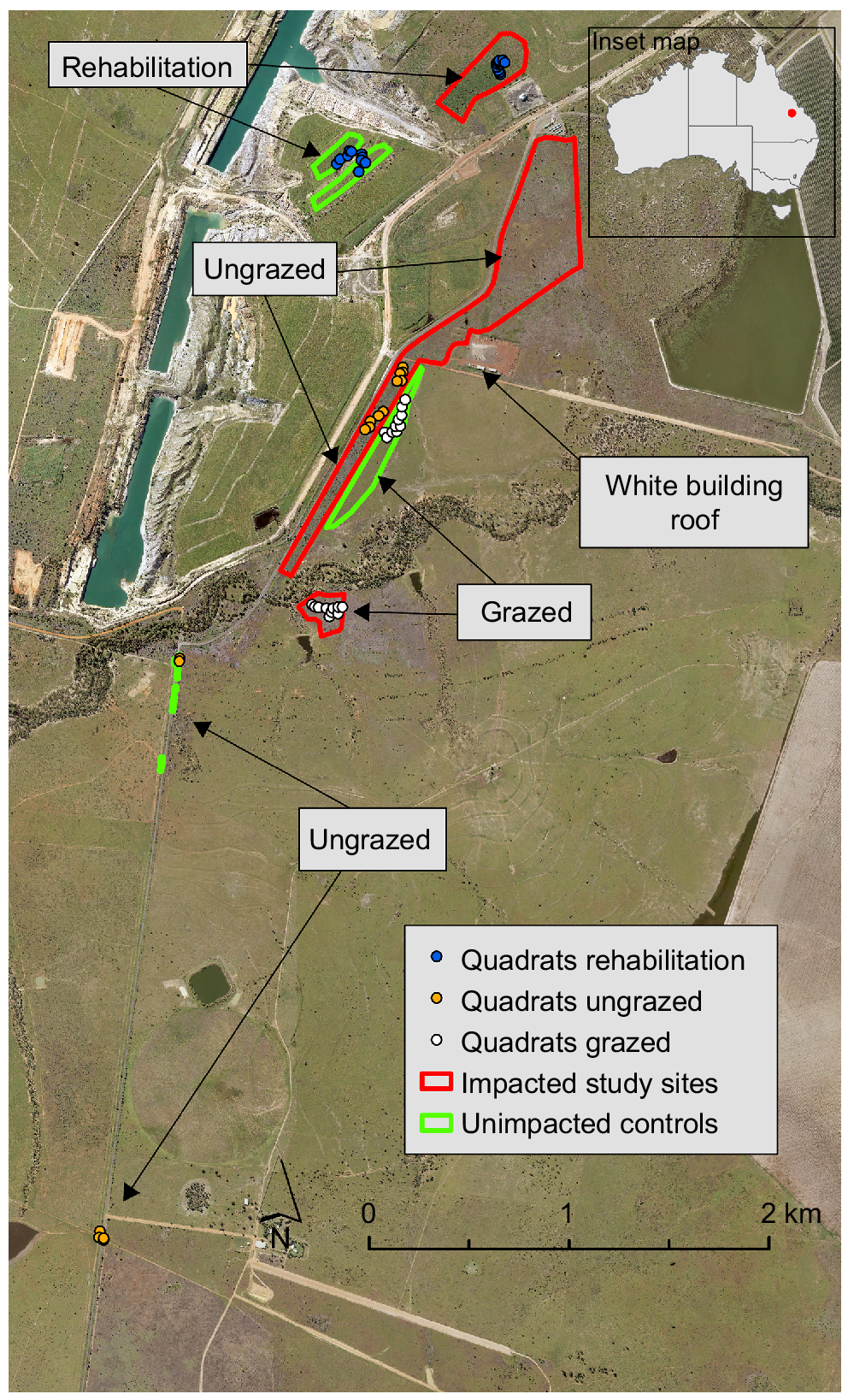
The study site is located in central Queensland, Australia, approximately 40 km east of the regional centre of Emerald (Fig. 1). The climate in the area is described by the Köppen classification as subtropical (BOM 2022), with a distinct wet (November–March) and dry season (April–October), and a mean annual rainfall of 614 mm (BOM 2021). The region experienced a significant pasture dieback event that was first noted on the ground by mine workers in 2018 and was seen to spread throughout local paddocks during 2019.
Study site showing location of rehabilitation, ungrazed and grazed polygons and quadrats (n = 10 for each land use except for rehabilitation where n = 20). Base image is May 2019 aerial and pasture dieback can be seen in the imagery as grey-brown pasture.
The soils in the study area are predominantly cracking clay vertosols (Humboldt Land System Land Unit 4), grading in the south to sand or loam over sodic clay – Sodosols, Kurosols (Monteagle Land System Land Unit 3) on the southern side of the Nogoa River (Gunn 1967) (Supplementary Fig. S1).
We used aerial imagery and detailed personal knowledge of the location to digitise polygons representing areas impacted and unimpacted by PD, subject to three different land uses: (1) ungrazed pasture, (2) grazed pasture and (3) rehabilitation after mining. We aimed to select study areas with the most consistent spatial and temporal coverage of imagery including avoidance of cloud shadows and image edges. We also attempted to select impacted and unimpacted (controls) polygons as geographically close as possible to minimise bias associated with differences in soils, topography and the climatic variables of rainfall and temperature (Fig. 1).
Identification of areas impacted by PD
The unimpacted (control) polygons in ungrazed areas were limited to roadsides and road verges and were dominated by buffel grass, as identified through aerial imagery and ground truthing (Fig. 1). Multiple small polygons totalling 0.2 ha were used to capture ungrazed, unimpacted areas due to the limited available area. As the aerial imagery extent in 2020 and 2021 did not cover the southern polygons, a smaller polygon selection covering 0.15 ha was used for the final two aerial GLI (green leaf index) time-series assessments. The aerial imagery was assessed to ensure that the selected polygon areas were not impacted by PD, grazing or other disturbances such as slashing or fire. A significantly larger polygon area of 42 ha of ungrazed roadsides was chosen to represent the PD-impacted area (Fig. 1). Although a comparison of different-sized ungrazed polygon areas may be deemed problematic, a large area of ungrazed land impacted by PD was justified to obtain a representative capture of the size and spread of the PD outbreak. It was also not possible to obtain a larger area of ungrazed, unimpacted land in the aerial imagery provided, because the majority of the ungrazed areas visible in the imagery were impacted by the PD event.
The grazing polygon representing PD impact was 5 ha in size and the unimpacted area was 6 ha. The impacted polygon was chosen to maximise available area while avoiding cloud shadow that was present to the south-west of the image in December 2019 (Fig. 1). Note that the grazing-impacted area was not covered in the 2020 and 2021 aerial images and is therefore not included in the green leaf index time series for these dates.
The rehabilitation polygon representing the impacted area was 8 ha in size, and the unimpacted area totalled 5 ha (Fig. 1). Both rehabilitation areas are reshaped spoil landforms following open-cut coal mining. These consisted of a mix of Permian and Quaternary spoils that were topsoiled to a depth of 30 cm, deep ripped, and then seeded with a mixture of native and exotic pasture, forb and shrub species. The rehabilitation was seeded between 2004 and 2007, with the focus areas for the study being the 2006 rehabilitation (Fig. S2). The two rehabilitation areas were completed as part of the same rehabilitation program in 2006 and therefore share many similarities, including slope gradient, topsoil quality, seed mix and supplier, and establishment pattern.
Both the impacted and unimpacted sites have had previous disturbances since site establishment. Notably, the 2006 unimpacted areas experienced a fuel reduction burn in October 2016, followed by light grazing between February 2017 and October 2017 (83 steers for 240 days). The site received follow-up moderate–light grazing between February 2018 and April 2018 (195 Brahman steers for 47 days) and finally, a second fuel reduction burn in September 2020.
In contrast, the impacted rehabilitation site experienced a lightning strike and small fire in February 2018. The area burnt was small (<1 ha) and was located in the 2007 rehabilitation, to the north of our quadrat locations (Figs 1 and S2).
The rehabilitation within the study area was assessed using recognised ecological monitoring methods by a consultant employed by the mine in 2014 and a repeat measure in 2020. In 2014, the area was reported to be dominated by buffel grass, butterfly pea (Clitoria ternatea L.) and burgundy bean (Macroptilium bracteatum Nees & Mart.). In 2020, the monitoring report noted that PD was present and was reducing buffel grass health on the landform delineated as the impacted site but was not noted in the unimpacted rehabilitation. Although the historical comparison shows some management differences between the unimpacted and impacted areas, the use of the unimpacted control remains valid for the intentions of this study and represents an area that has not been previously affected by PD. Interestingly, since the presence and or severity of dieback can be related to grazing intensity and level of pasture utilisation, this may have been a preventative factor for the unimpacted area.
Remote sensing
Aerial imagery was captured as part of routine mine site operational monitoring. The imagery varied in terms of spatial and temporal quality and coverage, with a pixel size ranging from 12 to 25 cm for the seven captures between 2015 and 2021. Images were supplied as .ecw (enhanced compression wavelet) files that were converted to .tif (tagged information format), clipped to the study area and georeferenced to the 2017 image with a root mean sqaure error RMSE <10 cm and digital numbers from 0 to 255.
Since the aerial imagery was limited to RGB bands, the green leaf index (GLI) was chosen to reflect changes in greenness of pasture in the visual spectrum (Eqn 1). The GLI has been shown to effectively measure vegetation changes in aerial imagery (Louhaichi et al. 2001). We extracted the mean GLI and standard deviation of the impacted areas and unimpacted controls for each land use polygon and plotted the delta GLI as a time series (Eqn 2). The divergence of delta GLI trajectories below zero indicates a period of decreasing greenness and potential PD occurrence, whereas an increase above zero suggests an increase in vegetation greenness compared the unimpacted control sites.
We compared the aerial delta GLI time series with delta GLI calculated using Planet, Sentinel-2 and Landsat satellite imagery on a corresponding time frame. Planet imagery was downloaded as a surface reflectance product and has a positional accuracy of <10 m RMSE (PlanetLabs 2022). Each Planet capture consists of four bands: red, green, blue and near-infrared covering the following bandwidths: 464–517 nm, 547–585 nm, 650–682 nm and 846–888 nm respectively. The orthorectified top-of-atmosphere Sentinel-2’s imagery of the study areas was obtained from Google Earth Engine Data Catalogue (https://developers.google.com/earth-engine/datasets/catalog/COPERNICUS_S2_HARMONIZED) via the Google Earth Engine Python client library (https://github.com/google/earthengine-api). We used a minimum cloud threshold of 20% for both Sentinel-2 and Landsat to filter out cloudy images. To ensure that the spectral variation from solar and atmospheric differences between captures of aerial images were not contributing to the trends observed, we also extracted the mean GLI values from a large building visible in the aerial imagery containing a white roof and plotted these values over time (Fig. 1).
Aerial imagery was processed using ArcGIS Pro V 3.0.2 (ESRI) and R Studio (R Core Team 2020) and the packages raster (Hijmans 2024) and ggplot (Wickham 2016).
Classification of imagery
We performed supervised machine learning classification on the aerial images using random forest (RF) in order to identify the spatial spread and PD recovery at the study sites (Breiman 2001).
Each aerial image was composited to create a 4-band raster (red, green, blue, green leaf index) and eight cover classes were selected using manual aerial photographic interpretation (API) techniques. This method involves manually selecting points from the imagery that represent cover classes to calibrate and validate the modelling (Jensen 2014). The classes chosen included bare ground (white colour), bare ground (brown colour), bare ground (asphalt), pasture dieback, healthy pasture, tree/shrub, canopy shadow and water. Separate API datasets were generated for each image class, with the numbers of points for each class varying depending on the API assessment (Table 1). The R Studio caret package was used for the RF classification (Kuhn 2021), which randomly splits the API dataset into 70% calibration and 30% validation. The number of trees (ntree) and the number of variables randomly sampled (mtry) are important hyperparameters of the RF model, which were set to 1000 and 20 respectively (Abdi 2020). Following classification, PD areas were converted to polygons, dissolved, and areas were calculated for each time step to determine the rate of spread and the recovery for each time step.
| Overall classification (eight classes) | PD class accuracy | Healthy ground veg class accuracy | Tree/shrub class accuracy | |||||||
|---|---|---|---|---|---|---|---|---|---|---|
| Image date | OMA (%) | Kappa | #Validation points | PA (%) | UA (%) | PA (%) | UA (%) | PA (%) | UA (%) | |
| 24 December 2015 | 80 | 76 | 297 | NA | NA | 60 | 66 | 70 | 68 | |
| 1 April 2017 | 88 | 82 | 548 | 96 | 85 | 96 | 89 | 43 | 71 | |
| 1 March 2018 | 92 | 90 | 838 | 94 | 90 | 95 | 96 | 88 | 90 | |
| 5 May 2019 | 82 | 77 | 1095 | 91 | 88 | 87 | 80 | 56 | 66 | |
| 31 December 2019 | 88 | 85 | 755 | 90 | 92 | 91 | 85 | 99 | 100 | |
| 28 December 2020 | 92 | 90 | 989 | 96 | 86 | 94 | 96 | 91 | 86 | |
| 1 December 2021 | 90 | 89 | 433 | 92 | 97 | 99 | 94 | 72 | 84 | |
| All combined | 80 | 75 | 13,744 | 79 | 83 | 80 | 84 | 68 | 63 | |
Error matrices for each year are located in Tables S1–S9. Note that OMA is overall mapping accuracy, PA is produced accuracy and UA is user accuracy.
In addition to developing a RF model for each image in the time series, we also trained one RF model on all the API training data points using the R package randomForest (Liaw and Wiener 2002). This was to assess the application and generalisability of the RF method over multiple years, seasons and images. For this, all API data points from each image were aggregated, and the RF algorithm was run to determine the accuracy of the predictions along with variable importance. Note that this classification was not applied to any of the images.
Error matrices were used to calculate the accuracy of the individual classes and the overall accuracy for each time-step along with the Kappa statistic, showing the overall agreement between the API and classified raster (Jensen 2005). Overall mapping accuracy measures the proportion of correctly classified pixels across all classes, providing an overall assessment of the classification performance. The Kappa statistic accounts for the inherent variability and randomness in classification outcomes, providing a more robust measure of classification accuracy. To assess the accuracy of the individual classes we evaluated the producer accuracy and user accuracy. Producer accuracy (PA) indicates the ability of the algorithm to accurately identify and include relevant pixels within the target class, whereas user accuracy (UA) represents the algorithm’s ability to accurately exclude irrelevant pixels from the target class. For error matrices see Tables S1–S9.
Weather dataset
Temperature and rainfall data were captured by a weather station situated on the mine site and by the Bureau of Meteorology (BOM) weather station located in the nearby regional town of Emerald. The BOM station records daily rainfall and temperature from 1992 to present and the data are publicly available via the BOM website. The mine site records daily rainfall and temperature from 2009 to present. We used data from both weather stations to plot monthly and seasonal trends across the time series, with particular interest in the period when PD was first identified in the imagery. We calculated the following: (1) total monthly rainfall, (2) mean monthly maximum temperature, (3) mean monthly minimum temperature, (4) highest monthly temperature, and (5) lowest monthly temperature. For each year, we calculated the percent change for each month from the long-term mean to detect any observable trends in the data.
Ground data
Ground surveys were conducted between 7 July 2022 and 10 July 2022 to validate the aerial imagery classifications and relate the vegetation recovery observed in the imagery with a number of ecological metrics. Within each land-use polygon, stratified random points were allocated and ten 1 × 1 m quadrats were recorded in each impacted and unimpacted control site for each land use area, with the exception of rehabilitated areas where n = 20 for impacted and unimpacted sites. Species richness, percent contributions to cover and biomass for each species were recorded in each quadrat, along with the percentage cover of live vegetation, dead vegetation, bare ground, detached litter and vegetation colour (red/purple, yellow, dry golden, dead grey). Dry weight biomass of vegetation was estimated in each quadrat using the dry-weight rank method (Haydock and Shaw 1975; McKenna et al. 2017). Field photos of each quadrat were captured, and quadrat locations were mapped using a Leica GNSS (global navigation satellite system) with RTK (real-time kinematic) corrections so that each point was <10 cm accuracy. The northwest corners of each quadrat were mapped, and the quadrats were aligned in a north–south direction.
Quadrats in rehabilitated areas were located in sites that were seeded in 2006 for the impacted areas and unimpacted controls (Fig. S2). Historical ecological monitoring reports show that both areas were dominated by three buffel grass cultivars. There are several commonly sown Buffel grass cultivars in central Queensland and there is mounting evidence to suggest that cultivars American and Gayndah are more susceptible to PD compared to cultivar Biloela (MLA 2023). Cultivar Biloela is easily identified due to its taller height and larger tiller and tussock size, but American and Gayndah are difficult to separate without adequate flowering material. As cultivars American and Gayndah are relatively equally susceptible to PD, for the purpose of this study these cultivars were aggregated. Cultivar Biloela is moderately tolerant to PD (MLA 2023), so was identified and treated in the analysis separately. The seeding mix of 2006 rehabilitation indicates a mix of cv. American and cv. Gayndah as well as a mix of ‘three varieties’ with no additional detail.
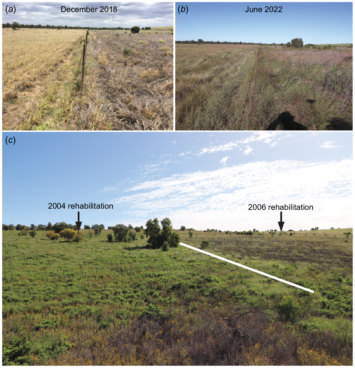
The selected ungrazed sites were associated with fenced-off roadside areas. PD was first noticed in the roadside area seen in Fig. 1, and ground photos taken in 2018 show that the area was dominated by buffel grass, mostly cultivars American/Gayndah (Fig. 2a).
Field photos of the study site: (a, b) show PD in the impacted ungrazed area of buffel grass (right side of fenceline) and the absence of PD in the unimpacted grazed area (left side of fenceline). December 2018 photo by Stuart Buck and June 2022 photo by Phillip McKenna. (c) Impacted rehabilitation showing two age classes. The 2004 rehabilitation is dominated by butterfly pea and mixed Acacia species, whereas the 2006 rehabilitation is dominated largely by yellow-flowering Crownbeard, which can also be seen in the foreground. Photo by Phillip McKenna, June 2022.
Field data were compiled and analysed using R (R Core Team 2020) using the RStudio interface and packages vegan (Oksanen et al. 2022), rstatix (Kassambara 2023) and ggplot2 (Wickham 2016) to compare mean species richness and biomass of the impacted and unimpacted areas within each ungrazed, grazed and rehabilitation land use. Data were tested for normality using the Shapiro–Wilk test, homogeneity of variance using Levene’s test and when data met the assumptions, a nonpaired t-test was used to compare the means between control and impacted locations. When the required conditions were not met, we used the Wilcoxon test for unpaired samples to determine the statistical significance.
Nonmetric Multidimensional Scaling (nMDS) was used to statistically compare the floristic variation patterns of the impacted and unimpacted areas within ungrazed, grazed and rehabilitation using PRIMER-E v 6.1.15 (Minchin 1987; Anderson et al. 2008). This was completed using (1) species presence/absence and (2) species contribution to percent cover data. Presence/absence data were analysed using the R vegan package with the Jaccard dissimilarity index, and contribution to percent cover was analysed using the Bray–Curtis dissimilarity index. Both indices evaluate the dissimilarity of vegetation communities, with a stress level less than 0.2 equating to a reasonable approximation of the patterns in the data. Species that were significant to the patterning (P < 0.05) were represented as vectors and cluster analysis (group average) was used to group the various communities by their similarity. Vector plots (radiating lines) using Pearson correlations were overlayed on the plots to demonstrate the species presence/absence variations driving the trend changes. The direction and length of the vector lines indicate the nature and strength of the relationship between individual species presence/absence and the ordination axis (Anderson et al. 2008).
See Fig. S3 for a workflow of the project.
Results
Remote sensing GLI time series
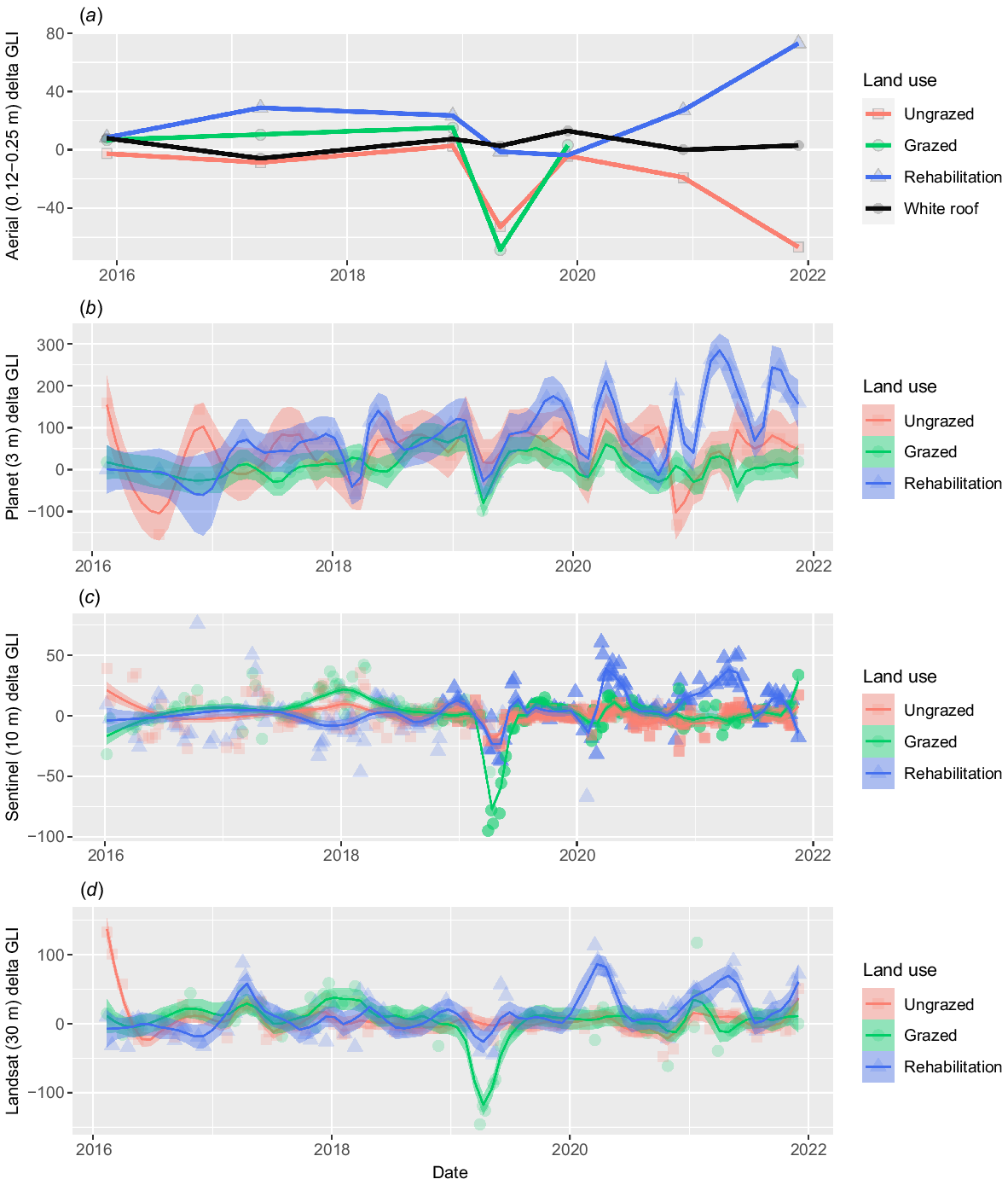
The analysis of the delta green leaf index from various imagery sensors effectively demonstrates the seasonal trends and decline in pasture health in ungrazed, grazed, and rehabilitated areas (Fig. 3). Aerial imagery successfully detected PD occurrences, including capturing the peak impacts in May 2019. Aerial imagery was also successful at detecting pasture regreening, with the grazed areas experiencing a 770% increase in the green leaf index between May and December 2019. Notably, the aerial imagery detected a significant increase in greenness within the rehabilitation areas by the end of 2021, and a reduction in greenness in ungrazed locations due largely to an increase in bare area, which satellite sensors failed to capture. These trends suggest that the GLI can add considerable value to RGB aerial imagery for the monitoring of pasture health including observing PD occurrence and pasture recovery.
Delta green leaf index (impacted – unimpacted) values using four sensors: (a) aerial, (b) Planet, (c) Sentinel-2, and (d) Landsat imagery. Mean white roof values in (a) show minimal variation, indicating that trends in the aerial imagery are not driven by differences in solar and atmospheric changes between captures. Planet GLI values were corrected for white roof due to variation in GLI values. Refer to Figs S7 and S8 for charts by individual land-use area.
Random forest model training
Table 1 provides the classification results recorded during the random forest model training, including the accuracy of the land cover identification across various image dates. The overall map accuracies (OMA) ranged from 80% to 92%, demonstrating the algorithm’s effectiveness in accurately classifying land cover. Notably, very high accuracies for the PD class, ranging between 79% and 97%, highlight the algorithm’s proficiency in identifying and distinguishing PD-affected areas.
The error matrices revealed areas of spectral confusion, particularly between the healthy ground vegetation and tree/shrub classes, leading to lower producer accuracies (PA) and user accuracies (UA) in specific time periods such as December 2015, April 2017, and May 2019. Furthermore, confusion between PD and asphalt was observed in certain image years (Tables S1–S9), emphasising the similarity in colour tones between PD and certain shades of grey associated with asphalt on road surfaces.
The analysis also revealed inaccuracies in detecting temporal variations. For instance, the class accuracies were relatively lower on 24 December 2015, 1 April 2017, and 5 May 2019, suggesting potential challenges in detecting and classifying PD depending on seasonal and phenological conditions. However, the accuracies overall indicated reliable results, with the algorithm performing well in distinguishing PD-affected areas and healthy ground vegetation.
Aerial imagery classification
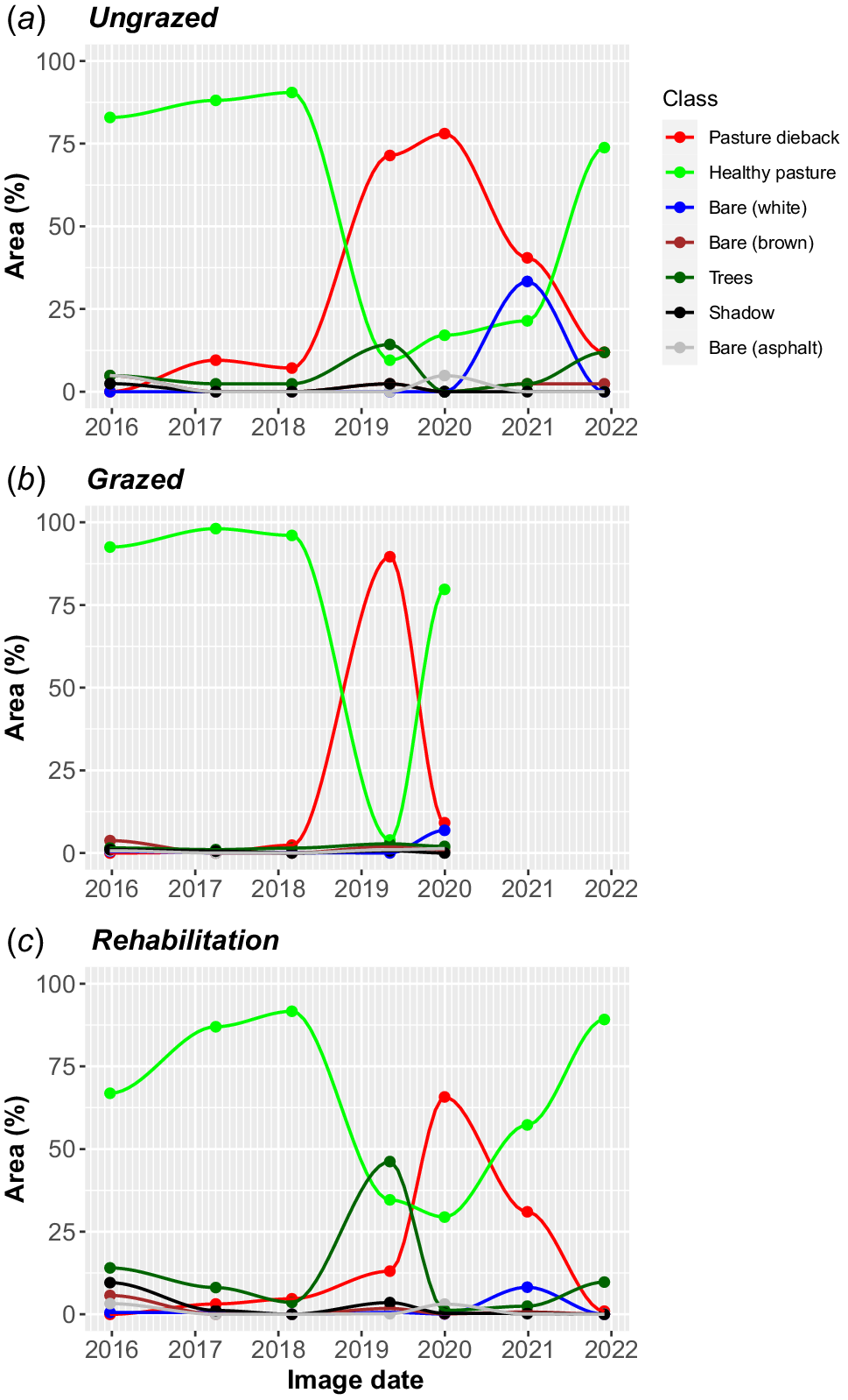
The classification of aerial imagery using the trained RF models revealed notable changes in PD and healthy vegetation class areas across seven image dates (Fig. 4). In May 2019, the maximum extent of PD occurred in the grazed polygon, reaching 90% coverage, whereas for ungrazed and rehabilitation sites, the peak coverage occurred in December 2019 at 78% and 66% respectively (Fig. 4). The rate of spread of PD was fastest in ungrazed areas at 1.88 ha month−1 (4.5% of polygon area per month) compared with rehabilitation and grazed at 0.54 ha month−1 (6.7%) and 0.19 ha month−1 (3.8%) respectively (Table 2). Interestingly, PD cover declined earlier and more rapidly in grazed areas (−0.31 ha month−1) over an 8 month period, in contrast to ungrazed and rehabilitated areas, which took almost 2 years to return to predisturbance levels (Table 2). Fig. 4 also highlighted some of the RF spectral errors and class confusion noted in the error matrices. For example, RF model confusion between trees and healthy pasture classes in the May 2019 classification is most apparent in ungrazed and rehabilitation impacted polygons.
Timelines of percent land cover classes as defined by random forest classifications for: (a) ungrazed impacted, (b) grazed impacted, and (c) rehabilitation impacted study areas. Note the longer residual of PD on ungrazed and rehabilitated areas compared with grazed.
| Date comparison | Change (months) | Ungrazed | Grazed | Rehabilitation | ||||||||
|---|---|---|---|---|---|---|---|---|---|---|---|---|
| Change (ha) | ha month−1 | % polygon month−1 | Change (ha) | ha month−1 | % polygon month−1 | Change (ha) | ha month−1 | % polygon month−1 | ||||
| Pasture dieback | December 2015 to April 2017 | 15.47 | 4 | 0.26 | 0.62 | 0.007 | 0.0005 | 0.0091 | 0.25 | 0.02 | 0.21 | |
| April 2017 to March 2018 | 11.13 | −1 | −0.09 | −0.21 | 0.063 | 0.01 | 0.11 | 0.13 | 0.01 | 0.14 | ||
| March 2018 to May 2019 | 14.33 | 27 | 1.88 | 4.49 | 2.706 | 0.19 | 3.78 | 0.68 | 0.05 | 0.59 | ||
| May 2019 to December 2019 | 8.00 | 2 | 0.25 | 0.60 | −2.493 | −0.31 | −6.23 | 4.28 | 0.54 | 6.69 | ||
| December 2019 to December 2020 | 12.10 | −15 | −1.24 | −2.95 | – | – | – | −2.82 | −0.23 | −2.91 | ||
| December 2020 to December 2021 | 11.27 | −12 | −1.07 | −2.54 | – | – | – | −2.44 | −0.22 | −2.71 | ||
| Green pasture | December 2015 to April 2017 | 15.47 | 3 | 0.19 | 0.46 | 0.17 | 0.01 | 0.22 | −0.48 | −0.03 | −0.39 | |
| April 2017 to March 2018 | 11.13 | 1 | 0.09 | 0.21 | −3.04 | −0.27 | −5.45 | −0.36 | −0.03 | −0.41 | ||
| March 2018 to May 2019 | 14.33 | −34 | −2.37 | −5.65 | 0.12 | 0.01 | 0.17 | 3.46 | 0.24 | 3.02 | ||
| May 2019 to December 2019 | 8.00 | 3 | 0.38 | 0.89 | 2.34 | 0.29 | 5.86 | −3.66 | −0.46 | −5.72 | ||
| December 2019 to December 2020 | 12.10 | 2 | 0.17 | 0.39 | – | – | – | 0.11 | 0.01 | 0.11 | ||
| December 2020 to December 2021 | 11.27 | 22 | 1.95 | 4.65 | – | – | – | 0.59 | 0.05 | 0.66 | ||
Highlighted grey cells represent peak changes in PD occurrence.
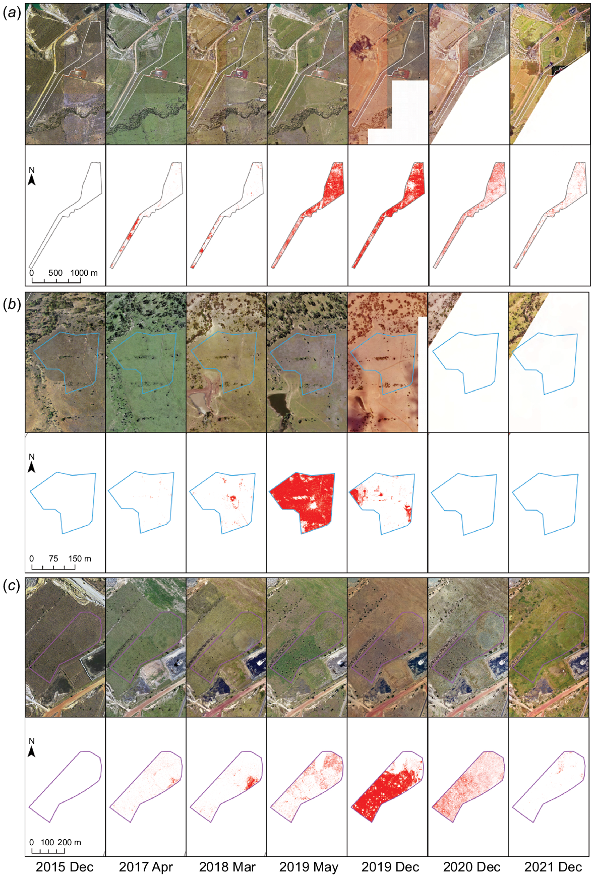
Fig. 5 visually illustrates the intricate spread patterns of PD within the affected polygons of ungrazed, grazed, and rehabilitated land use areas. The onset of PD infection traces back to April 2017, and its rapid expansion unfolds over time, with the ungrazed polygon displaying a more prolonged symptomatic period compared to the grazed and rehabilitation areas.
Timeline of aerial imagery and corresponding PD emergence and spread in impacted areas including (a) ungrazed (42 ha), (b) grazed (5 ha) (Note that there was no image coverage in 2020 and 2021), and (c) rehabilitation (8 ha).
The results support our hypothesis that remote sensing techniques have the capacity to measure PD emergence, spread and recovery in pasture systems in central Queensland. A range of sensors including aerial imagery using the GLI was able to demonstrate a decline in pasture greenness associated with PD emergence and spread and this imagery was successfully classified to measure rate of PD spread and pasture regreening.
Weather
Fig. 6 shows the trends for mean monthly rainfall, and temperature variables derived from the Mine Site weather station, and the BOM weather station located in Emerald, Qld. A number of key observations were apparent when the weather data were compared to long-term means. Firstly, the July 2016 (winter) monthly rainfall totals increased by 400% and 600% compared to the long-term averages for the mine site and BOM station respectively. This amounts to an increase of 2.8 and 3.7 standard deviations from the long-term mean (Fig. 6a). Secondly, the mean minimum monthly temperatures for winter increased relative to long-term means by 25% in 2016 and 30% in 2017. Minimum temperatures increased to a higher extent compared to maximum temperatures (Fig. 6b). Thirdly, the lowest monthly temperatures surpassed their long-term means by up to 100% for winter months, noticeably higher than the highest monthly temperature (Fig. 6c) and finally, the distinctive pattern of warmer night-time temperatures extends throughout 2016–2021 with notably higher than average winter night-time temperatures (Fig. 6b, c).
Percent change in monthly values compared to long-term monthly averages for (a) monthly rainfall totals taken from the mine site and Emerald BOM stations. July 2016 represents 2.8 and 3.8 standard deviations from the long-term mean respectively, (b) mine site weather station mean maximum and mean minimum and (c) mine site weather station highest and lowest monthly temperature. PD occurrence was first observed in the imagery in 2017 and spread throughout the sites. See Figs S5 and S6 for monthly temperature records for the Emerald and Blackwater BOM stations.
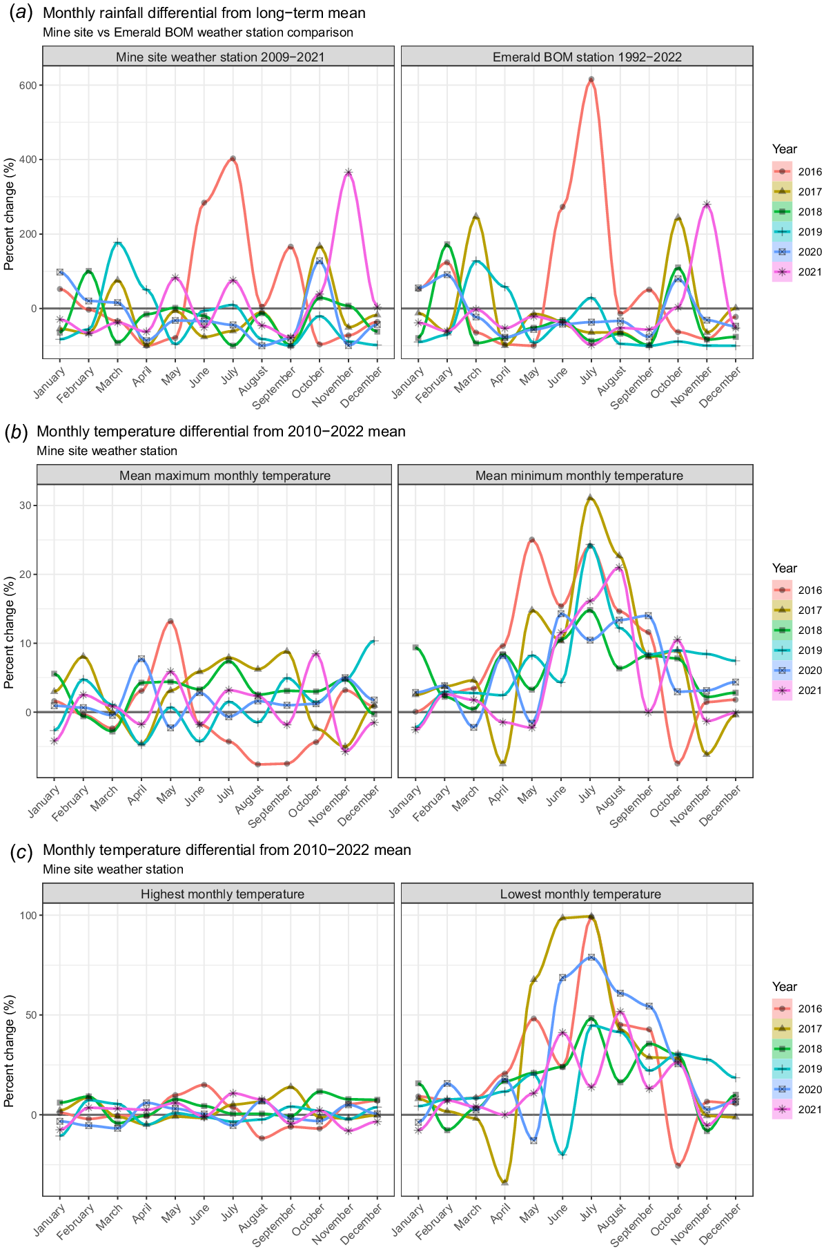
Fig. S4 presents the timeline of the mine weather station dataset from 2010 and highlights a shift into warmer winter temperatures in 2016 that continued throughout the period when PD was active. The BOM stations in Emerald and Blackwater further corroborate these temperature trends, exhibiting significant increases in winter night-time temperatures in 2016 and 2017. However, although the night-time temperatures showed considerably more variation compared to daytime temperatures, a number of winter months were colder; particularly 2018 winter night-time temperatures, which were colder than average at the Emerald and Blackwater BOM sites, suggesting that the mine weather station trend may be localised (Figs S5 and S6).
Ground surveys
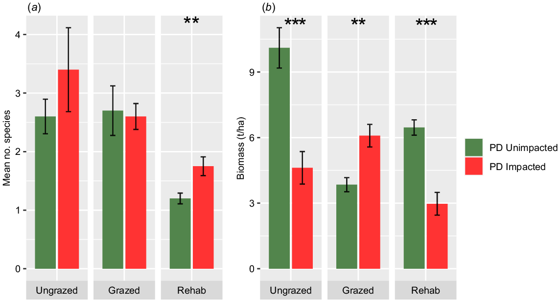
The results of the ground survey indicated that the average number of species per square metre was greater in quadrats affected by PD for ungrazed and rehabilitated land uses (P < 0.05) at 3.4 and 1.75 species m−2 respectively, compared to unimpacted control sites, which recorded 2.6 and 1.2 species m−2 respectively. For grazed quadrats, the results were similar for both unimpacted and impacted sites at 2.7 and 2.6 species m−2 respectively (Fig. 7a). In terms of understory biomass dry matter weights, the mean values for grass and forbs were higher in unimpacted control quadrats for ungrazed and rehabilitated locations (P < 0.001) at 10.1 and 6.5 t ha−1, respectively, compared to 4.6 and 3 t ha−1 in impacted sites. In contrast, the biomass was higher in impacted grazed areas (P < 0.01) compared to unimpacted controls, with a mean of 6.1 and 3.8, respectively (Fig. 7b).
(a) Species richness means ± s.e. and (b) mean ± s.e. dry-weight biomass for areas with and without PD under each land use. *P < 0.05, **P < 0.01, ***P < 0.001.
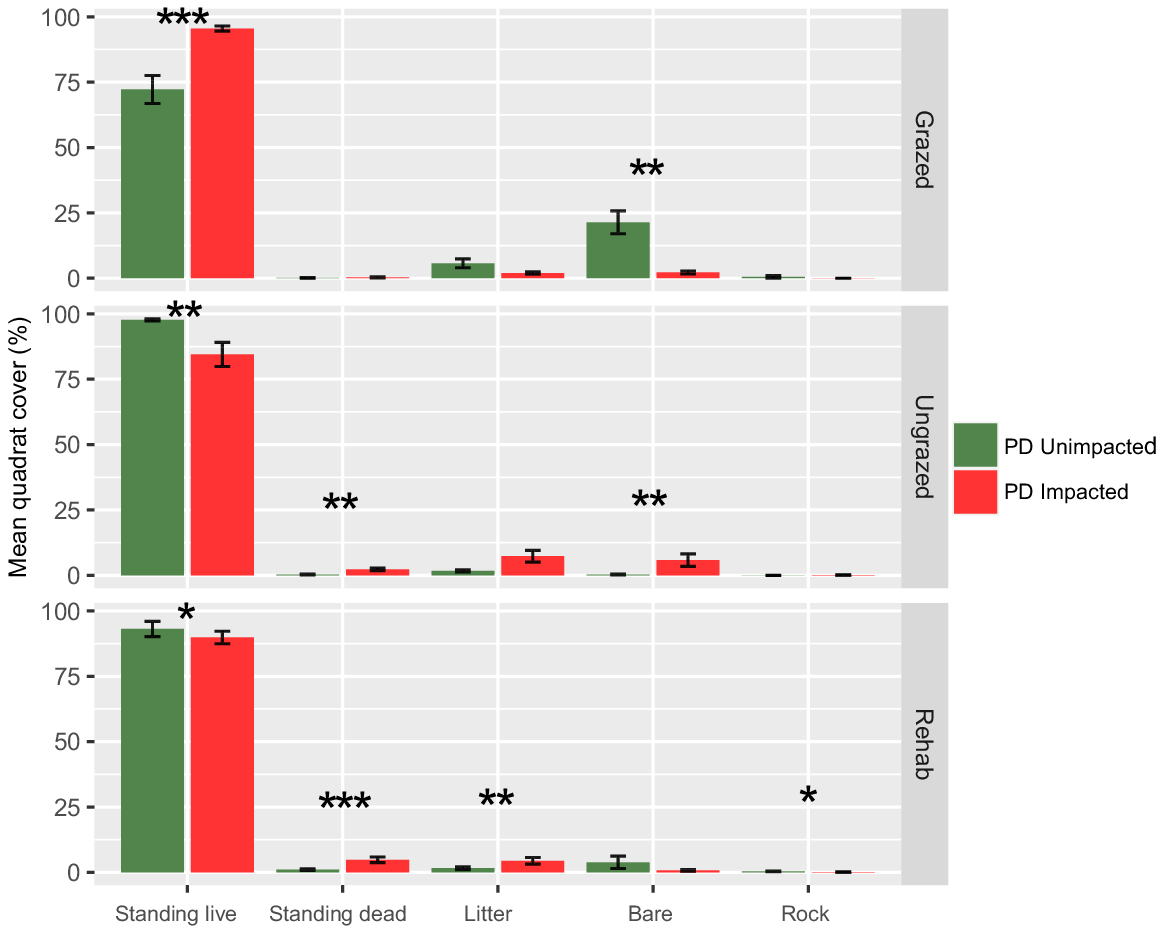
Multiple differences between the control and impacted sites are apparent when comparing the mean quadrat cover estimates (Fig. 8). Standing live cover in grazed locations was significantly higher in impacted quadrats (P < 0.001) with a mean cover of 96% compared to 72% in unimpacted control quadrats. Interestingly, bare area was higher in unimpacted controls at 21% compared to 2% in impacted quadrats (P < 0.01) in the grazed areas. Both ungrazed (P < 0.01) and rehabilitation (P < 0.05) showed similar cover trends for live vegetation cover, with unimpacted control quadrats recording significantly higher mean values compared to impacted quadrats.
Mean quadrat cover ± s.e. for grazed, ungrazed and rehabilitation areas *P < 0.05, **P < 0.01, ***P < 0.001.
Statistical summary tables are located in Tables S10–S12 and significance test results are located in Tables S13–S15.
Ordination plots show the ecological differences between PD impacted and unimpacted quadrats for species presence/absence (Fig. 9a–c).
nMDS ordination plots based on species presence/absence using Bray–Curtis similarity for ungrazed quadrats (a), grazed quadrats (b) and rehabilitation quadrats (c). Species vectors indicate those that are significantly contributing to the observed patterns. PD effects were was significant for all plots (P < 0.001).
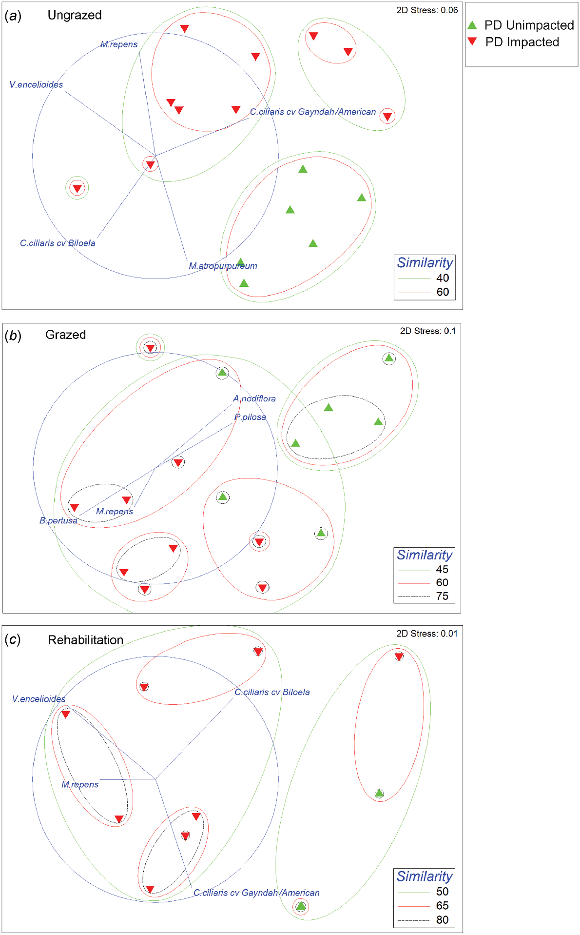
In general, all graphs showed that impacted sites recorded a significantly different species composition to unimpacted control sites (Table 3 and 4). In all land uses, species such as Verbesina encelioides (Cav.) Benth. & Hook. f. ex A. Gray (Crownbeard) and Melinis repens (Willd.) Zizka (Red Natal Grass) were recorded in the impacted quadrats but absent from the control sites (Table S16).
| Land use | PD | r2 | Pr(>r) | Significance | |
|---|---|---|---|---|---|
| Ungrazed | Impact vs unimpacted controls | 0.444 | 0.001 | *** | |
| Grazed | Impact vs unimpacted controls | 0.436 | 0.001 | *** | |
| Rehabilitation | Impact vs unimpacted controls | 0.601 | 0.001 | *** |
| Land use area | Species | nMDS1 | nMDS2 | r2 | Pr(>r) | Significance | |
|---|---|---|---|---|---|---|---|
| Ungrazed | C. ciliaris cv. Biloela | −0.860 | −0.509 | 0.672 | 0.001 | *** | |
| C. ciliaris cvv. Gayndah/American | 0.451 | 0.892 | 0.663 | 0.001 | *** | ||
| M. atropurpureum | −0.892 | 0.451 | 0.796 | 0.001 | *** | ||
| M. repens | 0.949 | −0.313 | 0.747 | 0.001 | *** | ||
| V. encelioides | 0.428 | −0.903 | 0.826 | 0.001 | *** | ||
| Grazed | A. nodiflora | 0.987 | 0.158 | 0.692 | 0.002 | ** | |
| B. pertusa | −0.998 | 0.058 | 0.557 | 0.004 | ** | ||
| C. cuneata | −0.352 | 0.935 | 0.393 | 0.009 | ** | ||
| P. pilosa | 0.993 | −0.110 | 0.554 | 0.001 | *** | ||
| S. spinosa | 0.100 | 0.994 | 0.469 | 0.006 | ** | ||
| V. encelioides | 0.027 | 0.999 | 0.341 | 0.046 | * | ||
| Rehabilitation | C. ciliaris cv. Biloela | 0.160 | 0.987 | 0.832 | 0.001 | *** | |
| C. ciliaris cvv. Gayndah/American | −0.938 | −0.346 | 0.866 | 0.001 | *** | ||
| M. repens | 0.354 | −0.935 | 0.202 | 0.017 | * | ||
| V. encelioides | 0.883 | −0.468 | 0.878 | 0.001 | *** |
Ungrazed impacted quadrats were significantly dissimilar to control quadrats (P < 0.001) and this difference was driven by the presence of a number of species at impacted sites, including Verbesina encelioides, Melinis repens, Desmodium campylocaulon (F.Muell. ex Benth.) H.Ohashi & K.Ohashi, Rhynchosia minima (L.) DC., Minuria leptophylla DC. and Alternanthera nodiflora R.Br. By contrast, the unimpacted control quadrats were largely dominated by Cenchrus ciliaris cv. Biloela and Macroptilium atropurpureum (DC.) Urban (Table 4, Fig. 9a).
Grazed impacted sites were significantly dissimilar to unimpacted controls (P < 0.001) due to the increasing presence and cover of Bothriochloa pertusa (L.) A. Camus, whereas unimpacted controls were dominated by Cenchrus ciliaris cvv. Gayndah/American, Portulaca pilosa L. and Alternanthera nodiflora (Table 4, Fig. 9b). Although the grazed quadrats showed a different species mix for control and impacted sites, the cover contribution was largely defined by two species: C. ciliaris cvv. Gayndah/American and B. pertusa (Fig. S9B).
Rehabilitated impacted sites were significantly dissimilar to control sites (P < 0.001), with Verbesina encelioides contributing to the presence and the cover in the impacted sites. C. ciliaris cvv. Gayndah/American and C. ciliaris cv. Biloela were significant in the unimpacted control quadrats (Table 4, Fig. 9c).
The results support our hypothesis that there are significant differences within each land use, between impacted sites and controls. Differences were observed between impacted and unimpacted quadrats for species richness, biomass, cover and composition; suggesting that a significant floristic shift occurs in buffel grass pastures following symptoms of PD.
Discussion
Pasture Dieback (PD) is predominately impacting exotic grasses throughout eastern Queensland. The long-term implications for the occurrence of PD at the property scale are not well understood, and although vegetation recovery on impacted sites across the state has occurred, the rates of recovery and changes in species composition are understudied (Buck et al. 2022a). This study showed the spatial, temporal and ecological dynamics of PD at a local scale in terms of spread patterns and subsequent recovery. We used remote sensing techniques to calculate the GLI and then classified areas of PD and healthy vegetation. To our knowledge this is the first study to quantify the rate of spread of PD in a number of land use areas. The remote sensing component was supported by ground validation and demonstrated that vegetation richness, biomass, cover and composition in PD impacted areas were significantly different to vegetation in unimpacted control areas.
This study demonstrated the utility of high spatial resolution remote sensing to map and monitor PD and illustrates the potential future mapping of pasture health using a range of remotely sensed products, including the GLI. In general, PD was distinguishable using manual API and random forest classifiers when healthy grass tussocks were green and actively growing (e.g. 2019 image), rather than when pastures were hayed off and mature (e.g. 2015 image). The colour contrast between healthy vegetation versus that affected by PD was greatest in May 2019, which was when the GLI trajectories showed maximum deviation between control and impacted mean values. Interestingly, this also corresponds with a shift to rainfall excess following a period of rainfall deficit (Fig. S10). Buffel grass pastures are valued for their drought and grazing tolerance (Hodgkinson et al. 1989; Williams and Baruch 2000) and in the local area the species has been described colloquially as a ‘resurrection plant’ – one that can remain alive during extreme dry conditions. It is not unusual for entire landscapes to show extensive haying off, but the colour is often golden-brown (e.g. December 2015 image) compared to the grey colour of PD-affected tussocks (e.g. May 2019 image) (Buck 2021). In contrast to hayed off grass, PD is characteristically patchy in its spatial distribution and has been observed affecting selected areas while other areas or paddocks remain green and healthy (MLA 2020). This is observed in the 2019 images where the ungrazed roadsides showed a clear delineation between impacted and healthy pasture (Fig. S11).
Although PD was first observed by mine staff in 2018, the high-resolution aerial imagery classifications showed that PD was first present in April 2017 in the ungrazed roadside areas and was visibly identifiable in the pasture by a unique dark, red colour (Figs 5a and S11). PD was shown to spread throughout ungrazed roadside areas in a patchy manner, turning the pasture a characteristic grey colour as it progressed along a fenceline as buffel grass tussocks died. By the time of the May 2019 image capture, PD was observed to be widespread throughout the ungrazed areas, while grazed pasture directly adjacent to (other side of the fenceline) appeared to be unaffected. In the years following, an increase in bare area was recorded prior to vegetation reestablishment as noted in the 2021 capture and image classification (Fig. 4a, c). Although PD was detected in all three land-use areas in the December 2018 image, there was a time delay of approximately 7 months for peak impact in the rehabilitated study area compared to the ungrazed and grazed paddocks.
Interestingly, the timing of the initial 2017 detection of PD follows a period of increased winter night-time temperatures and higher winter rainfall in 2016 and corresponds with a 200% increase in March 2017 rainfall at the mine site. The 2016 year was a period where one of the strongest El Niño events in Australia dissipated and conditions for high rainfall resulted in the wettest May to September on record (BOM 2017). If the increase in winter night-time temperatures along with higher than average winter rainfall patterns have played a role in the establishment and spread of PD at this site, it is possible to speculate that PD may have been caused by either (1) an increase in plant stress due to disrupted night-time biochemical processes, (2) an increase in populations of plant pests or pathogens (e.g. mealybugs) due to favourable breeding and feeding conditions or (3) a combination of both. A recently-published study has shown an increase in Rubber Leaf Fall Disease was linked with increasing trends in mean temperatures in Southeast Asia (Azizan et al. 2023), which could support this hypothesis. However, our warmer winter night-time temperature theory would need to hold across a regional scale; and although a recent remote sensing study found an increasing 2015–2020 temperature trend across 187 PD study sites in Queensland and NSW, these changes were not statistically significant (Nguyen and Grace 2021). Whereas the BOM sites in Emerald and Blackwater showed increased variation in night-time temperatures, the mine site winter temperatures were all notably warmer, suggesting that a localised affect might have occurred.
This study supports previous knowledge that pastures with low (or no) utilisation by cattle are commonly affected by pasture dieback (Brazier and Buck 2021). The most striking example of this was the ungrazed impacted site that was rapidly and severely impacted by PD, while the grazed paddock just metres away appeared to be unimpacted. The rehabilitated pastures also support this finding, since the unimpacted controls experienced grazing and controlled burning in the years prior to the PD occurrence, whereas the impacted rehabilitation experienced minimal disturbance.
Our results demonstrate the importance of ground validation surveys in remote sensing studies (Nagai et al. 2020). Although remote sensing metrics showed regreening (suggesting vegetation recovery) following the 2017–2019 symptoms, the quadrats at the impacted sites recorded significant differences in species richness, biomass, cover and composition compared to the quadrats on the unimpacted control sites (Fig. S12). Pasture recovery may be from the few surviving tussocks, or if pastures completely die, from germinating seeds within the soil seedbank. Given that the ungrazed and rehabilitation impacted sites recorded higher mean species richness and lower mean biomass it is likely that these sites recovered mostly from the soil seedbank.
Management implications
Although previous studies have tested and demonstrated the resilience of rehabilitation established after mining to fire disturbance (McKenna et al. 2019), there have been no peer-reviewed studies on the challenges to rehabilitated estates from biotic disorders such as pasture dieback. This study demonstrated a level of recovery following PD, but also shows the potential for ecological shifts in community composition following disease that has the potential to alter rehabilitation trajectories (Grant 2006). The recent legislative reforms in Queensland require mine sites to account for their residual risk, which is defined as the probability that remedial action will be required following rehabilitation completion (Environmental Protection Act). The Queensland Government recently released an interim guideline for the assessment of residual risks (DES 2020), however, the credible risk events have a clear focus on engineering risks (e.g. geotechnical, geochemical risks etc.) rather than environmental and ecological risks. Interestingly, the 2004 and 2006 rehabilitation that was impacted by PD is now dominated by Clitoria ternatea (Butterfly Pea), Macroptilium atropurpureum (Siratro), Verbesina encelioides and other forbs (Figs 2 and S12), whereas unimpacted controls are buffel grass dominated. Although these results suggest a level of residual risk to future landholders, the risks are not exclusively related to the rehabilitation, since unmined pastures and analogue areas are also impacted by PD to a similar level. Given that PD-impacted sites show vegetation recovery over 2 years, should this trend continue, it is expected that rehabilitation can still meet its agreed end land use, including the completion criteria for minimum ground cover, therefore satisfying regulators who are responsible for Environmental Authority surrender and lease relinquishment.
This study suggests that the management of roadside verges and unused pasture areas is important to protect the broader region from PD effects. It is possible that PD emergence was simultaneous across multiple areas, but our analysis suggests that the first emergence was in an area of ungrazed roadside pasture. This area also contains a low density of shrubs including Acacia salicina Lindl., Santalum sp., Terminalia oblongata F.Muell. and Bauhinia sp. which would be difficult to slash and would require selective grazing or low intensity burning to manage fuel loads and maintain tussock vigour.
Limitations
Several limitations in this study are worth describing to provide context for the results. Firstly, without preimpact (baseline) ground surveys, we assume that the control sites represent a similar vegetation assemblage to the impacted sites before the PD occurrence. This also includes the assumption that the vegetation at the control sites has not changed significantly for the duration of the study. Traditionally a study such as this would aim to use the before-after-control-impact (BACI) study design (Elzinga et al. 1998). Although we can use a baseline and BACI with the remote sensing data, we do not have preimpact ground data to compare vegetation changes. Historical monitoring reports were available for rehabilitated areas and indicated that the impacted block was dominated by buffel grass (unspecified cultivar) and Siratro, but the grazed and ungrazed areas do not have any preimpact ground floristic data. Of particular note, the selection of ungrazed controls were limited due to the lack of unimpacted and ungrazed areas within the study site. As a result, the ungrazed controls along the roadsides were dominated by Cenchrus ciliaris cv. Biloela, which may not represent the predisturbance assemblage of the ungrazed impacted sites and may have been a factor in the protection of these areas from the PD onset. The impacted ungrazed areas were dominated by C. ciliaris cvv. American/Gayndah, with a mix of other species including C. ciliaris cv. Biloela.
Secondly, due to time limitations, we were constrained by the number of quadrats used in the ground sampling assessment. Ten quadrats in control and ten in impacted sites for grazed and ungrazed areas and twenty quadrats for the rehabilitation areas provided enough replicates for a statistical comparison, but statistical power could be improved with a greater number of replicates in future studies.
Thirdly, a limited land area was available for particular combinations of land use and PD impact. This restricted comparison among land use areas as well as the comparison across PD status (control vs impacted). The ungrazed control areas selected from road verges were the only areas that could reliably be selected as ungrazed and unimpacted. In a region dominated by cattle grazing, ungrazed control areas were spatially restricted. We exerted effort to locate accessible sites, but the road verges were the only areas that could reliably be selected as ungrazed and unimpacted.
The classification algorithms such as random forests can be fine-tuned to improve the classification results (Abdi 2020). Although the class accuracies were high, there were a number of false positives that the algorithm produced during the classification process (Fig. S11). This is partly a function of the RGB limitations and can be noted by the confusion of asphalt with PD, based purely on visible colour, rather than the traditional use of longer wavelengths and reflectance spectra of near-infrared or short-wave infrared, which produce higher reflectance values based on plant cell walls and water content in plant leaves (Jensen 2014). We didn’t include any manual filtering or postprocessing of the classification outputs since we were only interrogating small parcels of land and clipped classified polygons to each area. Future remote sensing projects could conduct additional cleaning and filtering to generate a more accurate classified data set.
Finally, it is possible over a 7-year period that all the sites were impacted with unknown interventions including slashing, different grazing intensities, fire and herbicide applications, which could influence the susceptibility to PD and vegetation recovery. We were limited to what could be viewed in the imagery and site knowledge. Understanding these influences would require a different study with an expanded scope and increased temporal coverage of the sites, which is not currently available.
Conclusion
The use of high spatial and temporal aerial imagery has resulted in the initial detection and mapping of pasture dieback spread and subsequent vegetation in our study site in central Queensland. We demonstrated that the green leaf index can be used to detect pasture changes either through aerial imagery or broader spatial scale satellites from Planet, Sentinel-2 or Landsat. Classification of RGB imagery resulted in high overall map accuracies and class accuracies for PD and a trained random forest model using aggregated API training points suggests that the RF model can be used effectively across a range of phenological, and seasonal grass curing conditions. Although remote sensing indices indicated pasture recovery, field validation showed that impacted pastures shifted from buffel grass-dominated, to forb-dominated communities with significantly different species mix, biomass and cover conditions.
Declaration of funding
Phillip McKenna received a grant from the Australian Coal Industry’s Research Program (ACARP) grant number C33045.
References
Abdi AM (2020) Land cover and land use classification performance of machine learning algorithms in a boreal landscape using Sentinel-2 data. GIScience and Remote Sensing 57, 1-20.
| Crossref | Google Scholar |
Amarasingam N, Gonzalez F, Salgadoe ASA, Sandino J, Powell K (2022) Detection of white leaf disease in sugarcane crops using UAV-derived RGB imagery with existing deep learning models. Remote Sensing 14, 6137.
| Crossref | Google Scholar |
Azizan FA, Astuti IS, Young A, Abdul Aziz A (2023) Rubber leaf fall phenomenon linked to increased temperature. Agriculture, Ecosystems & Environment 352, 108531.
| Crossref | Google Scholar |
BOM (2017) Annual climate statement 2016. Bureau of Meteorology, Australian Government. Available at http://www.bom.gov.au/climate/current/annual/aus/2016/
BOM (2021) Climate statistics for Australian locations. Bureau of Meteorology, Australian Government. Available at http://www.bom.gov.au/climate/averages/tables/cw_034038.shtml
BOM (2022) Climate classification maps. Bureau of Meteorology, Australian Government. Available at http://www.bom.gov.au/jsp/ncc/climate_averages/climate-classifications/index.jsp?maptype=kpngrp#maps
Boschma S (2020) What is pasture dieback? NSW Department of Primary Industries. Online Webinar May 2020. Available at https://www.youtube.com/watch?v=K8KPZWBde6g
Brazier N, Buck S (2021) Characterising pasture dieback: analysis of the current situation in northern Australia. In ‘Proceedings of the 33rd Biennial Conference of the Australian Association of Animal Sciences. Vol. 33’. (Ed. D Mayberry) (Australian Association of Animal Sciences) Available at https://futurebeef.com.au/wp-content/uploads/2023/10/Characterising-pasture-dieback-analysis-of-the-current-situation-in-northern-Australia_Brazier_2021.pdf
Breiman L (2001) Random forests. Machine Learning 45, 5-32.
| Crossref | Google Scholar |
Buck S (2017) Pasture dieback: past activities and current situation across Queensland (2017). Project Report. (Department of Agriculture and Fisheries: Brisbane, Qld) Available at http://era.daf.qld.gov.au/id/eprint/6521/1/Pasture-dieback-past-activities-and-current-situation-across-Queensland-2017.pdf
Buck S (2020) Pasture dieback in Queensland. NSW Department of Primary Industries, Qld Department of Agriculture and Fisheries. Online Webinar May 2020. Available at https://www.youtube.com/watch?v=RAL4-AS0K3M
Buck S, Hopkins K, Brazier N, Thomas K, Moravek T, Landsberg L, Fletcher J, Stockwell P, Jones P (2022a) Grazier engagement to increase knowledge, skills and ability to combat pasture dieback. (Meat & Livestock Australia: Sydney, NSW) Available at https://www.mla.com.au/research-and-development/reports/2023/b.pas.0511---grazier-engagement-to-increase-knowledge-skills-and-ability-to-combat-pasture-dieback/
Buck S, Ouwerkerk D, Gilbert R, Miles M, Grice K, Giblin F, Crew K (2022b) Comprehensive diagnostic analysis of pastures affected by dieback. (Meat & Livestock Australia: Sydney, NSW) Available at https://www.mla.com.au/contentassets/0695b89ef0694aa9ba623924da4f3a1c/b.pas.0509-ms-6-final-report_.pdf
DAF (2023a) Pasture dieback – signs and symptoms. Queensland Department of Agriculture and Fisheries. Available at https://futurebeef.com.au/resources/pasture-dieback-signs-and-symptoms/
DAF (2023b) Pasture dieback or pasture rundown? Queensland Department of Agriculture and Fisheries. Available at https://futurebeef.com.au/resources/pasture-dieback-or-pasture-rundown/
DES (2020) Residual risk assessment guideline – interim. (Queensland Department of Environment, Science and Innovation: Brisbane) Available at https://environment.des.qld.gov.au/__data/assets/pdf_file/0019/214354/era-gl-residual-risk-assessment.pdf
Government of Queensland (2018) Managing residual risks in Queensland. Discussion Paper. Part of the financial assurance framework reform package. (Government of Queensland: Brisbane) Available at https://environment.des.qld.gov.au/__data/assets/pdf_file/0036/88857/managing-residual-risks-discussion-paper.pdf
Graham G, Conway M (1998) Some sick Buffel. TGS News and Views. Tropical Grassland Society of Australia 14, 6.
| Google Scholar |
Grant CD (2006) State-and-transition successional model for bauxite mining rehabilitation in the Jarrah forest of Western Australia. Restoration Ecology 14, 28-37.
| Crossref | Google Scholar |
Gunn RH (1967) Lands of the Isaac-Comet Area, Queensland, Part VII Soils of the Isaac-Comet Area. Available at https://medium.com/@arifwicaksanaa/pengertian-use-case-a7e576e1b6bf
Hauxwell C (2022) B.PAS.0004. Final report. Biology of pasture mealybug and identification of natural enemies. (Meat and Livestock Australia: Sydney, NSW) Available at https://eprints.qut.edu.au/233434/1/B.PAS.0004_Final_report_MLA.pdf
Hauxwell C, Buck S, Driver F (2022) Monitor for mealybugs now. Feedback Magazine. Meat & Livestock Australia 24. Available at https://www.flipsnack.com/mlafeedback/meat-livestock-australia-feedback-magazine-spring-2022/full-view.html
Haydock KP, Shaw NH (1975) The comparative yield method for estimating dry matter yield of pasture. Australian Journal of Experimental Agriculture and Animal Husbandry 15, 663-670.
| Crossref | Google Scholar |
Hernandez-Santin L, Rudge ML, Bartolo RE, Erskine PD (2019) Identifying species and monitoring understorey from UAS-derived data: a literature review and future directions. Drones 3, 9.
| Crossref | Google Scholar |
Hijmans R (2024) raster: Geographic Data Analysis and Modeling. R package version 3.6-28, https://rspatial.org/raster.
Hodgkinson KC, Ludlow MM, Mott JJ, Baruch Z (1989) Comparative responses of the Savanna grasses Cenchrus ciliaris and Themeda triandra to defoliation. Oecologia 79, 45-52.
| Crossref | Google Scholar | PubMed |
Kassambara A (2023) rstatix: pipe-friendly framework for basic statistical tests. R package version 0.7.2. 105. Available at https://cran.r-project.org/web/packages/rstatix/rstatix.pdf
Kuhn M (2021) caret: classification and regression training. R package version 6.0-90. Available at https://doi.org/10.1201/b17172-15
Larrinaga AR, Brotons L (2019) Greenness indices from a low-cost UAV imagery as tools for monitoring post-fire forest recovery. Drones 3, 6.
| Crossref | Google Scholar |
Lechner AM, Foody GM, Boyd DS (2020) Applications in remote sensing to forest ecology and management. One Earth 2, 405-412.
| Crossref | Google Scholar |
Liaw A, Wiener M (2002) “Classification and Regression by randomForest.”. R News 2(3), 18-22 Available at https://CRAN.R-project.org/doc/Rnews/.
| Google Scholar |
Louhaichi M, Borman MM, Johnson DE (2001) Spatially located platform and aerial photography for documentation of grazing impacts on wheat. Geocarto International 16, 65-70.
| Crossref | Google Scholar |
Makiela S, Harrower KM (2008) Overview of the current status of buffel grass dieback. Australasian Plant Disease Notes 3, 12-16.
| Crossref | Google Scholar |
McKenna PB (2018) Measuring rehabilitation responses to fire using transects and remote sensing. Master of Philosophy Thesis, The University of Queensland, Australia. Available at https://doi.org/10.14264/uql.2018.859
McKenna P, Glenn V, Erskine PD, Doley D, Sturgess A (2017) Fire behaviour on engineered landforms stabilised with high biomass buffel grass. Ecological Engineering 101, 237-246.
| Crossref | Google Scholar |
McKenna PB, Erskine PD, Glenn V, Doley D (2019) Response of open woodland and grassland mine site rehabilitation to fire disturbance on engineered landforms. Ecological Engineering 133, 98-108.
| Crossref | Google Scholar |
McKenna PB, Lechner AM, Hernandez Santin L, Phinn S, Erskine PD (2022) Measuring and monitoring restored ecosystems: can remote sensing be applied to the ecological recovery wheel to inform restoration success? Restoration Ecology 31, e13724.
| Crossref | Google Scholar |
Minchin PR (1987) An evaluation of the relative robustness of techniques for ecological ordination. Vegetatio 69, 89-107.
| Crossref | Google Scholar |
MLA (2020) Pasture dieback: a management guide for producers and agronomists. (Meat & Livestock Australia: Sydney, NSW) Available at https://www.mla.com.au/globalassets/mla-corporate/research-and-development/documents/mla-pasture-dieback-manual.pdf
MLA (2023) How do I … select grass varieties tolerant to pasture dieback? (Meat & Livestock Australia: Sydney, NSW) Available at https://www.mla.com.au/globalassets/mla-corporate/research-and-development/documents/select-grass-varieties-factsheet-final-approved.pdf
Nagai S, Nasahara KN, Akitsu TK, Saitoh TM, Muraoka H (2020) Importance of the collection of abundant ground-truth data for accurate detection of spatial and temporal variability of vegetation by satellite remote sensing. In ‘Biogeochemical cycles: ecological drivers and environmental impact. pp. 223–244. (Wiley) doi:10.1002/9781119413332.ch11
Oksanen J, Simpson GL, Blanchet FG, Kindt R, Legendre P, Peter M, O’Hara RB, Solymos P, Henry M, Stevens H, Szoecs E, Wagner H, Barbour M, Bedward M, Bolker B, Borcard D, Carvalho G, Chirico M, Caceres M De, Durand S, Beatriz H, Evangelista A (2022) Vegan: community ecology package. R package version 2.5–7. Available at https://cran.r-project.org/web/packages/vegan/vegan.pdf [Accessed 17 April 2022]
PlanetLabs (2022) Planet imagery product specifications. Planet Labs Inc. pp. 1–100. Available at https://www.planet.com/products/satellite-imagery/files/Planet_Imagery_Product_Specs.pdf
PlanetLabs (2023) Real-time satellite monitoring with planet. Available at https://www.planet.com/products/monitoring/
R Core Team (2020) ‘R: a language and environment for statistical computing.’ (R Foundation for Statistical Computing: Vienna, Austria) Available at https://www.r-project.org/
Summerville WAT (1928) Mealy bug attacking Paspalum grass in the Cooroy district. Queensland Agricultural Journal 30, 201-209.
| Google Scholar |
Tamiminia H, Salehi B, Mahdianpari M, Quackenbush L, Adeli S, Brisco B (2020) Google Earth Engine for geo-big data applications: a meta-analysis and systematic review. ISPRS Journal of Photogrammetry and Remote Sensing 164, 152-170.
| Crossref | Google Scholar |
Thomson M (2019) Hidden Gems: an epidemiological investigation into the association of ground pearls with pasture dieback. Honours Thesis, The University of Queensland, Gatton, Qld, Australia. Available at https://doi.org/10.13140/RG.2.2.34427.13606
Thomson MB, Campbell SD, Young AJ (2021) Ground pearls (Hemiptera: Margarodidae) in crops and pastures: biology and options for management. Crop & Pasture Science 72, 762-771.
| Crossref | Google Scholar |
Ustin SL, Middleton EM (2021) Current and near-term advances in earth observation for ecological applications. Ecological Processes 10, 1.
| Crossref | Google Scholar | PubMed |
Wickham H (2016) ggplot2 – elegant graphics for data analysis (2nd Edition). Journal of Statistical Software 77, 1-3.
| Crossref | Google Scholar |
Williams DG, Baruch Z (2000) African grass invasion in the Americas: Ecosystem consequences and the role of ecophysiology. Biological Invasions 2, 123-140.
| Crossref | Google Scholar |