

Vegetation classification in south-western Australia’s Mediterranean jarrah forest: new data, old units, and a conservation conundrum
Sarah Luxton A E , Grant Wardell-Johnson A , Ashley Sparrow B , Todd Robinson C , Lewis Trotter C and Andrew Grigg D
A School of Molecular and Life Sciences, Curtin University, GPO Box U1987, Perth, WA 6845, Australia.
B Biodiversity Division, Environment and Climate Change Group, Department of Environment, Land, Water and Planning, PO Box 137, Heidelberg, Vic. 3084, Australia.
C School of Earth and Planetary Sciences, Curtin University, GPO Box U1987, Perth, 6845 WA, Australia.
D Department of Environmental Research, Alcoa of Australia Ltd, PO Box 172, Pinjarra, WA 6208, Australia.
E Corresponding author. Email: sarahjluxton@outlook.com
Australian Journal of Botany 69(7) 436-449 https://doi.org/10.1071/BT20172
Submitted: 6 January 2021 Accepted: 30 May 2021 Published: 28 July 2021
Journal Compilation © CSIRO 2021 Open Access CC BY
Abstract
Conservation reserve selection is guided by vegetation classification and mapping. New survey data and improvements in the availability of archived data through online data-sharing platforms enable updated classifications and the critique of existing conservation criteria. In the Northern Jarrah Forest Region of south-western Australia, percentage-based targets using ‘forest ecosystem units’ (15% of each unit) and the systematic conservation planning principles of ‘comprehensiveness, adequacy and representativeness’ underpin the State’s reserve network. To assess the degree of community-level heterogeneity within the forest ecosystem units, new survey data for the forest (30 000 plots) were classified using a non-hierarchical clustering algorithm. Results were assigned to the National Vegetation Information System, and community groups defined at the Association level (Level V). Significant community level heterogeneity was found, including 15 communities in the dominant ‘jarrah woodland’ unit, and 13 in the ‘shrub, herb and sedgelands’ unit. Overall, this research highlights limitations in the current reserve system, including the influence of scale on percentage-based targets and ‘representativeness’. A multi-scale approach to reserve selection, based on a quantitative, floristic, hierarchical classification system, would improve the level of scientific rigour underlying decision-making.
Introduction
A primary goal of natural resource management is to balance development with conservation. In Australia and internationally, conservation reserve networks are key to achieving this (Cabeza and Moilanen 2001; Rondinini and Chiozza 2010; Kullberg and Moilanen 2014; Morelli et al. 2020; Stralberg et al. 2020). Vegetation classification and mapping underpin networks and provide a scientific basis for decision making. However, challenges remain. Baseline data are missing because of poor survey coverage, whereas incomplete and inconsistent classifications prevent assessment at suitable scales (McKenzie et al. 1996; Jennings et al. 2009; Franklin 2013; Peet and Roberts 2013). New data and the centralisation of datasets provide platforms for improvement and are occurring internationally (VegBank, BIEN, sPlot), nationally (TERN Aekos) and at State and Territory levels (e.g. BioNET (New South Wales), COREVeg (Queensland), NatureMap (Western Australia), the Vegetation Site Database (Northern Territory); Benson 2008; Wiser and De Cáceres 2013; Chytrý et al. 2016; Faber-Langendoen et al. 2018; Gellie et al. 2018; Gibson 2018; Addicott and Laurance 2019; Bruelheide et al. 2019). Using these products to improve conservation assessment at multiple scales is key to improving decision-making.
Conservation decisions require targets (Bakker 2013). In Australia, this includes a continent-wide target of 17% of terrestrial ecosystems to be reserved, on the basis of the 2020 Convention on Biological Diversity’s Aichi Target 11 (www.cbd.int/aichi-targets/target/11). More specifically, the National Reserve Strategy’s (NRS) aim is a ‘comprehensive, adequate and representative’ (CAR) reserve system at the bioregional scale (JANIS 1997; Commonwealth of Australia 2010). The Interim Biogeographic Regionalisation for Australia (IBRA) and regional ecosystem units are the basis for CAR targets (Commonwealth of Australia 2010). This includes the pre-1750 extent of vegetation and examples of at least 80% of the number of regional ecosystems in each IBRA region (comprehensiveness) or subregion (representativeness).
Although IBRA and regional ecosystem units provide a general framework for setting CAR targets, limitations are evident, particularly for defining and measuring representativeness. Representativeness is ‘comprehensiveness considered at a finer scale’ (Commonwealth of Australia 2010, p. 10); however, how IBRA subregions (rather than regions) are used to determine representativeness and detect finer-scale heterogeneity is not clear. The definition of regional ecosystems is also generic, with scale being a critical factor:
Ecosystems, or a unique unit such as a vegetation community mapped at appropriate scales, comprising a recognisable floristic composition in combination with a substrate (lithology, geology layers) and position in the landscape, and including their component biota [Commonwealth of Australia 2010, p. 65].
Work that tests how data collection and analysis methods affect the quantification of heterogeneity and representativeness will improve the scientific underpinning of the NRS.
State and Territory land and vegetation databases and map products provide the basis for this work. New South Wales BioNet collection includes over 800 maps of varying resolution, coverage and currency (Benson 2008). Queensland has 20 years of Regional Ecosystem Mapping (Neldner et al. 2019) and scale is recognised as important for detecting true floristic heterogeneity (Wardell-Johnson et al. 2007). Victoria’s ecological vegetation classes (EVC) provide a range of units including mosaics, complexes, aggregates and generic wetland mapping units, which, in combination with bioregions, provide a bioregional conservation status (BRS) (databased in NatureKit 2.0). In Western Australia, state-wide mapping is at a 1 : 3 000 000 scale (Beard 1990; Shepherd et al. 2002; Beard et al. 2013). Broad floristic formations (forest ecosystem units) underpin the conservation reserve system, Regional Forest Agreement and Forest Management Plan (2014–2023; Department of Agriculture, Water and Environment 2019) (JANIS 1997; Commonwealth of Australia 1998; Government of Western Australia and the Commonwealth of Australia 1999; Conservation Commission of Western Australia 2013). Community-level mapping (1 : 5000–1 : 100 000) is available in some regions (Wardell-Johnson et al. 1989; Wardell-Johnson and Williams 1996; Mattiske and Havel 1997, 1998). This finer-scale mapping is used in development assessment, for determining offset targets, and informal reserve definition, but has not been fully incorporated into assessments of CAR for the conservation reserve system (JANIS 1997; Ecoscape 2002).
The Northern Jarrah Forest (NJF) region of south-western Australia provides a case study for investigating how community-scale data may influence CAR targets, including representativeness. A Mediterranean forest, the area has important commercial and conservation values, including as a major water catchment area for Perth (Petrone et al. 2010; Hughes et al. 2012; Wardell-Johnson et al. 2015). Alcoa of Australia Ltd (Alcoa) have collected 30 000 plots of floristic data since the 1990s (see Trotter et al. 2018 for full details). The dataset covers a restricted area at high resolution, enabling community mapping and comparison to the broad floristic formations currently used to set CAR conservation targets in the forest.
Here, we use the dataset to assess how an updated classification informs mapping and conservation targets across scales in the NJF. Our aim is to describe and understand vegetation heterogeneity and its implications for decision-making. To do this, we perform the following:
-
Classify the data at three scales and use remotely sensed environmental attributes and modelled climate data to describe results. Landscape position (upland and plateau v. valley floors) is predicted to drive vegetation differences at broad scales, with finer patterns driven by local topography and soil.
-
Assign groups to the hierarchical National Vegetation Information System (NVIS).
-
Compare the groups derived from this analysis to the units currently used for mapping and decision-making, and assess how results inform the representativeness of the reserve system in the NJF.
Materials and methods
Study site
The NJF has a Mediterranean climate, with an average annual rainfall of 1300 mm in the west, dropping to 600 mm inland and to the east (Havel 1975b; Gentilli 1989). A dry-sclerophyll system, it ranges from low woodlands in the north to open forests in the south (McKenzie 2008). The forest is significant globally, as Mediterranean ecosystems house a fifth of known vascular plant species in only 2% of the world’s land area. They are also one of the biomes predicted to experience the greatest biodiversity change over the next 80 years, through both climate and human land-use pressures (Sala et al. 2000; Klausmeyer and Shaw 2009; Cox and Underwood 2011; Moreira et al. 2019). The NJF also occurs in the South-western Australia Global Biodiversity Hotspot (Myers et al. 2000; Hopper et al. 2016). Vegetation patterns are characterised by subdued topography, rainfall and regular fire incidence (Burrows et al. 2019). The forest also has a history of logging and mining (1834–current) that has considerably affected structure (Calver and Wardell-Johnston 2004; Wardell-Johnson et al. 2015). Floristically, the forest overstorey is largely dominated by two tree species, namely, Eucalyptus marginata (jarrah) and Corymbia calophylla (marri), but it has a complex and diverse understorey (3096 taxa; Dell et al. 1989; see https://florabase.dpaw.wa.gov.au). Understorey vegetation has been described as a multidimensional continuum with semi-discrete community types (Havel 1975a).
The climatic and hydrological regimes of the forest are shifting in response to global warming; rainfall has decreased by 16% and temperature increased 0.4°C since the mid-1970s (Bates et al. 2008; CSIRO, State of the Climate 2020, see csiro.au/state-of-the-climate). This has led to decreased surface run-off (20–100%), falling water-tables and shifts from perennial to ephemeral streams (Petrone et al. 2010; Hughes et al. 2012; Zhang et al. 2016). High summer evapotranspiration offsets winter rainfall, which is predicted to further decrease under continuing climate change (CSIRO, State of the Climate 2020, see csiro.au/state-of-the-climate).
Floristic data
To meet statutory requirements, Alcoa has been collecting floristic data in the NJF for almost 30 years (1991–ongoing). Vegetation mapping now spans 432 km2 with 31 000 plots on a 120-m2 grid that follows ore exploration (Fig. 1). At each grid point, tree species were recorded in a 20-m radius and understory taxa in a 5-m radius. Cover-abundance (1–5) and stress (1–5) were scored (Mattiske 2012). Collected plant specimens were dried, fumigated and identified in accordance with the requirements of the Western Australian Herbarium (Mattiske 2012; see https://florabase.dpaw.wa.gov.au) and the conservation status of taxa were checked using current Government Gazette lists (see https://florabase.dpaw.wa.gov.au). Each plot in the dataset was also assigned a site vegetation type, which is the community-scale unit used for mapping in the forest (Havel 1975a, 1975b). Eleven types were described across the study area.

|
Environmental data
Environmental variables were collected at each plot, and included soil type, topography, outcrop type and amount, dieback (Phytophthora cinnamomi) presence or absence and impact, years since fire, log debris and number of tree stumps. Additional environmental variables were generated in the System for Automated Geoscientific Analyses (SAGA, ver. 2.1.2; Conrad et al. 2015) using NASA’s one arc-second (30 m) Shuttle Radar Topography Mission (SRTM) hydraulically enforced digital elevation model (DEM; Geoscience Australia 2011).
Topographic variables include distance to channel base network, which is calculated from an inverted DEM and negatively correlated with elevation (high valley-depth values indicate a larger distance from ridge lines, or lower valley position). Distance to valley depth is an inverted ridge-top distance. Curvature and convexity both measure the roundness or hollowness of a surface, with convexity indicating the number of convex shapes within a set radius, whereas curvature measures the convex or concavity of a slope. The SAGA wetness index (SWI) was used to represent flow across the study area. SWI is similar to the topographic wetness index (TWI; Beven and Kirkby 1979), but is based on a modified catchment-area calculation, which does not conceptualise flow as a thin film (Böhner et al. 2002).
Aspect in degrees was transformed to radians for further analysis (Roberts 1986). Northness (derived from cos(aspect)) has values close to 1 if the aspect is northward (or –1 if southward). Alternatively, eastness is a function of sin(aspect), with values close to 1 representing east-facing slopes. Environmental data were tested for collinearity using the package corrplot (Wei et al. 2017). Where correlation was more than 0.5 (positive or negative), one variable from the pair was removed (Fig. S1 of the Supplementary material). Removal was based on previous research and expert opinion regarding which environmental driver would be the most valuable when interpreting vegetation patterns (e.g. Havel 2000).
Data cleaning
A floristic information management system was developed to prevent data corruption and data-entry error, and to ensure that future data additions fit system requirements (Trotter et al. 2018). This included automating name updates through Max (the Western Australian Herbarium platform for sharing plant name updates, see https://www.dpaw.wa.gov.au/about-us/science-and-research/publications-resources/113-max-a-species-database-helper-for-windows). In addition to the technical data-cleaning process, 337 species were excluded from the original Alcoa species list because of data-entry errors, subspecies updates and incorrect species identification. Singletons (a single species record) and doubletons (only two species records) were also removed from the dataset for this analysis (186 species). Annuals, biennials, deciduous taxa such as most geophytes, and alien taxa were removed because surveys were not conducted consistently in the flowering season. In total, 435 species remained in the modified dataset for this analysis. Floristic data were summarised in R (ver. 3.4.2, see https://cran.r-project.org/bin/windows/base/old/3.4.2/) and species richness and Shannon diversity were calculated.
Algorithm choice
Cluster analysis was performed using the non-hierarchical algorithm ALOC in PATN (ver. 3.12, see https://patn.org/; Belbin 1984, 1987; Belbin and McDonald 1993). Non-hierarchical algorithms have benefits over hierarchical ones, because they ‘produce a single partition that optimises within-group homogeneity, instead of a hierarchical series of partitions optimizing the hierarchical attribution of objects to clusters’ (Legendre and Legendre 2012, p. 349). The goal is to obtain a direct representation of the relationships among objects, rather than a summary of the hierarchal relationships that optimise fusions (Belbin 1987; Legendre and Legendre 2012). The potential to re-allocate objects to any group in the partition at each iteration is another advantage of non-hierarchical models, and computing memory requirements can be lower, as an object–group, rather than object–object resemblance matrix is calculated (Legendre and Legendre 2012). Negatives include that users must pre-define the number of groups to be clustered and that the relationship between objects (usually shown by a dendrogram) can be difficult to visualise.
By calculating object–group, rather than object–object associations, the non-hierarchical algorithm ALOC is effective in clustering large datasets. The number of groups is pre-defined by the user and the number of iterations n–1 (n = sample size). The algorithm begins by allocating objects to a (suboptimal) set of seeds, starting with the first object in the dataset (although prior groups can also be used). It proceeds by taking each object, calculating the closest group and reallocating it to a closer group if more a homogenous option is found, until an overall optimal solution is reached (Belbin 1987). Overall, the algorithm is reasonably insensitive to seeds, and has been tested against hierarchical methods and shown to have a good recovery of clusters (Belbin and McDonald 1993).
Alternative non-hierarchical clustering algorithms that were investigated, but not selected for analysis, include k-means, partitioning around meoids (PAM), clustering large applications (CLARA), OPTPART and OPTSIL (MacQueen 1967; Kaufman and Rousseeuw 2009; Roberts 2015; Kassambara 2017). K-means is a commonly used unsupervised machine learning algorithm (Kassambara 2017). It classifies objects so that within cluster, similarity is maximised, and between-clusters it is minimised. There are several k-means algorithms; however, the standard one (Wong and Hartigan 1979) uses Euclidean distance, which is sensitive to outliers and not appropriate in data with many zeros, as is the case for many ecological datasets.
PAM (or k-medoids clustering) is less sensitive than is k-means to outliers and more likely to converge at a similar solution from different starting medoids (Kaufman and Rousseeuw 2009). However, PAM is considered suitable for at most 2000–3000 plots (R help file). CLARA is the recommended non-hierarchical alternative in R for larger datasets, but also uses Euclidean (or Manhattan) distance. Roberts (2015) stated an updated case for the use of non-hierarchical clustering with his algorithms OPTPART and OPTSIL. However, OPTSIL took 50 h of CPU time for 209 species and 424 sites (Intel I7 processor). Because this dataset has over 400 species and 30 000 sites, the computing time would have been large. Although high-performance computing provides solutions to this, fast desktop alternatives such as PATN (one simulation took an average of 20 min to complete) are a practical and effective alternative.
Cluster analysis and evaluation
For this study, a site by species matrix (31 087 sites; 435 species) was imported into PATN and the Data > Analysis option was selected. The pre-set menu of PATN splits analysis options by columns and rows. For rows, no association measure was selected, with non-hierarchical clustering (constant 2) and 99 final groups. Ninety-nine groups were selected to ensure that adequate community variation was captured, relative to the number of communities previously described for the study area (11). For columns, a two-step association measure was selected, with 21 groups, to display site by species relationships (constant 2). All evaluations were selected (details below). The analysis was run, and results were exported to Excel for further processing.
PATN has a range of summary statistics that can be exported from the cluster analysis and used to visualise the results. This includes row (sites) and column (species) group statistics. Column summary data show the mean value of a species association to a group centroid, with the most frequent species having the highest values, whereas row data capture the group and distance to centroid that a site belongs to. Row statistics were used to produce an object–group dendrogram, to show how groups are related to one another, whereas species scores (column statistics) were used in non-metric multidimensional scaling (nMDS) to display species–group relationships. Visual assessment of the dendrogram was used to determine the number of clusters (groups) for further interpretation and evaluation.
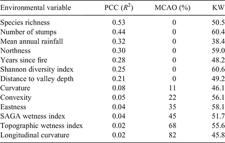
Cluster evaluation was performed using the inbuilt evaluation tools of PATN (Belbin 1993; L. Belbin, unbpul. data). These include the Kruskal–Wallis statistic, principal-component correlation (PCC) and Monte-Carlo attributes in an ordination (MCAO). Kruskal–Wallis is a non-parametric (rank-based) test. In PATN, environmental variables were used to determine a significant difference among groups, with higher values being the most discriminating (Kruskal and Wallis 1952). PCC fits environmental variables to the cluster solution in ordination space, using multiple linear regressions (each variable is fitted independently) and provides an R2 value for interpretation (Belbin 1993). MCAO tests the robustness of the PCC results. Using MCAO, environmental variables are re-allocated among objects (sites), the PCC linear regressions re-run 100 times and results compared with the true R2 value. Results show the number of R2 values that exceeded the true R2 value (percentage permuted R2 > actual R2), with values higher than 5 of 100 indicating that a significant correlation is unlikely (PATN help file). Because of the limitations in PATN for the visualisation of non-hierarchical results in ordination space, the results of the clustering (species group statistics) were exported and displayed using nMDS (with the Bray–Curtis index) in R using the package vegan (ver. 2.3.1, J. Oksanen, F. G. Blanchet, M. Friendly, R. Kindt, P. Legendre, D. McGlinn, P. R. Minchin, R. B. O’Hara, G. L. Simpson, P. Solymos, M. H. H. Stevens, E. Szoecs, and H. Wagner, see https://cran.r-project.org/web/packages/vegan/index.html).
Typology and comparison to previous classifications
Following visual interpretation and cluster evaluation, 2, 11, 30 and 77 groups were selected for further analysis. The 30-group partition was chosen to represent community-level patterns, based on expert interpretation. Because no synoptic table or fidelity measure options are available in PATN, species frequency per group was calculated to show the dominant (indicator) species for each group (Table S1). A NVIS-style description was developed for each community group (McKenzie 2008; NVIS Technical Working Group 2017). Several attributes required for a NVIS description were inferred, because data were not collected in the field (stratum cover, dominant growth form and average height). Cover was based on species frequency per group, whereas the dominant growth form was assigned using FloraBase (see https://florabase.dpaw.wa.gov.au/) species descriptions. Strata were assigned on the basis of growth form, including upper layer (U): trees; mid-layer (M): shrubs, small trees and monocots; and ground layer (G): small shrubs, grasses, sedges, ferns, cycads and herbs. Boxplots and nMDS with the Bray–Curtis index were used to visualise species–group and environmental associations for the 2- and 30-group partitions in R. Summary statistics from the cluster analysis for the 30-group partition (mean distance from group centroids for each species) were used as input for the nMDS ordination.
An analysis of the difference between previously mapped units and the current results was performed using a confusion matrix of the frequency of site occurrence between the two typologies (see the R script file in the Supplementary material). Because 11 community types had been previously described across the study area, an 11-group partition of the classification was used for the comparison. Finally, confusion statistics (commission, omission and overall accuracy) were calculated for the updated typology.
Results
Classification
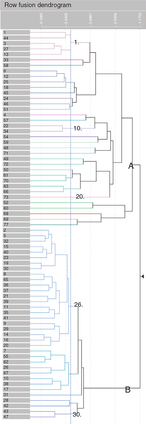
Overall, the classification identified two supergroups, representing the upland and riparian flora of the NJF (A and B, Fig. 2). These supergroups are heavily skewed; Supergroup B contains the majority of sites (95%) and species, with the largest subgroup (26) containing 404 species and 24 253 sites (Fig. 2, Table S1). Upland species dominate this supergroup (Table 1), reflecting their high abundance in the dataset (jarrah, marri and Macrozamia riedleii, interspersed with Xanthorrhoea preissii, Bossiaea aquifolium, Allocasuarina fraseriana, Persoonia longifolia and Pteridium esculentum). Species unique to the riparian supergroup (A, 1421 sites, Fig. 2) include Eucalyptus patens, Taxandria linearifolia, Banksia littoralis and Hypocalymma angustifolium, which are associated with valleys, stream banks and seasonally wet areas (see https://florabase.dpaw.wa.gov.au/). Key dominant species occur across both supergroups, notably jarrah, marri, X. preissii, M. riedleii and P. esculentum (Table 1, Table S3). Aspect, valley depth and convexity varied between the two supergroups, with riparian sites (A) being found lower in the landscape on less convex, north-east-facing slopes (Fig. 3). Species richness and the number of stumps (a measure of historic logging intensity) was also lower (Fig. 3).
|

|

|
At the community level (30 groups) Eucalyptus patens, E. rudis and E. megacarpa co-occur with the forest-wide dominants jarrah and marri in the upper stratum of riparian communities (Fig. S2, Table S3 of the Supplementary material). Mid-stratum species Trymalium ledifolium and X. preissii co-occur widely with both upland and riparian taxa. The major communities (26–30) were not well separated in ordination space, but 16 small groups (<20 sites) and uncommon taxa occurred as outliers, associated with restricted or distinct topographic features (Fig. 4). Kunzea micrantha (KUNMIC) and Aotus cordifolia (AOTCOR) are shrubs found in peaty soil, marshes and swamps, and K. micrantha forms a community with other riparian taxa including Melaleuca preissiana, E. megacarpa and Lepidosperma squamatum. The outlier Philydrella drummondii (PHDRU) is a perennial herb of freshwater swamps. Community 23 contains species associated with granite outcrops including the fern Cheilanthes austrotenuifolia (CHEAUS), Neurachne alopecuroidea (NEUALO) and Hakea petiolaris (HAKPET; FloraBase, see https://florabase.dpaw.wa.gov.au/). Several other outlier species are likely because of low records numbers or data-cleaning errors (e.g. E. microcorys and Stylidium calcaratum, an alien and annual species respectively; Fig. 4).

|
Overall, there were significant differences (MCAO < 5%) among the community groups in species richness, the number of stumps (a measure of logging disturbance), mean annual rainfall and aspect (northness; Table 2). Mean annual rainfall explained the most variation among groups (R2 = 0.32, MCAO = 0%), whereas northness (R2 = 0.3, MCAO = 0%) and years since fire (R2 = 0.28, MCAO = 0%) were also significant (Table 2). At the supergroup level, Supergroup B was associated with higher wetness and valley depth values (a negative corollary of elevation) on reduced slopes (Fig. 3, Table S2). Both eastness and northness were positive for Supergroup A (0.32, 0.35; indicating north-east-facing slopes) and were slightly negative in Supergroup B (–0.04, –0.03; indicating a very slight south-west-facing tendency; Fig. 3, Table S2).
|
Comparison to current mapping in the forest
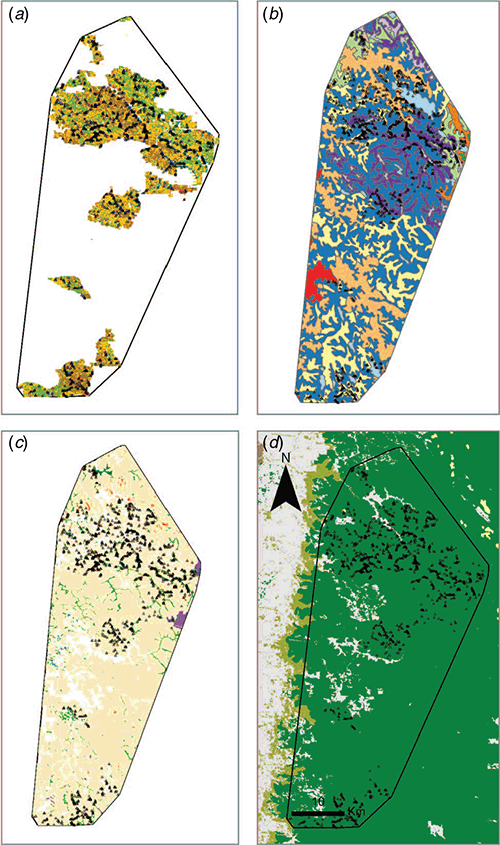
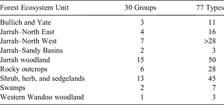
Nine forest ecosystem units have been mapped for the study area (Fig. 5c). Broadly, they are comparable to the supergroups, there being geographic overlap between Supergroup A and the non-dominant forest ecosystem units (e.g. shrub, herb and sedgelands), whereas Supergroup B corresponds to the jarrah–north-west unit (Fig. 5c). The community (30 group) and 77 type classifications showed additional heterogeneity not captured by the forest ecosystem units (Table 3). For example, jarrah woodlands contains 15 communities and 50 types, whereas the shrub, herb and sedgelands unit incorporates 13 communities and 45 types (Table 3). Alternatively, the western wandoo woodland unit corresponds with a single community and only two swamp communities were described for the larger swamp unit.
|
|
At the community scale, previous mapping for the forest has been conducted using site vegetation types (SVT), with 11 being described in the study area (Table 4, Fig. 5a). There is some overlap between previous mapping and an 11-group cut of the current classification, with the majority of historic types (SVT) clustering into one major and two minor groups (overall accuracy = 45%, Table 4). Over half of the SVTs are found in the S and T groups (64% of plots); however, the current 11-group classification is even more unbalanced, with 95% of plots falling into Group 11 and seven groups having <10 quadrats each (Table 4). Group 1 contains the largest proportion of historic types associated with wet and riparian conditions (A, C, W; Table 4).

|
Discussion
Reserve systems are a key societal tool for balancing development with conservation (Pressey et al. 2007; Volenec and Dobson 2020). Reserve selection in Australia is based on systematic conservation planning (with the goal of being CAR), and a percentage area, regional approach is used to define comprehensiveness and representativeness (Commonwealth of Australia 2010; Kukkala and Moilanen 2013). This study used the classification of a large floristic database (~30 000 sites) to define vegetation types at several scales and test the representativeness of current units. Overall, two large supergroups (upland v. riparian) and 30 communities were described. The community classification includes rarer types that occur in topographically distinct (e.g. granite outcrops) or riparian areas, within a matrix of commonly occurring species across the uplands and plateaus. Tests of representativeness found that up to 15 communities occur within the regional-level units currently used for decision-making. Results demonstrated that community-level heterogeneity is not adequately captured by the conservation reserve system. Although it currently meets national CAR targets, additions are required to meet the criteria of representative at the community scale.
Explaining heterogeneity
The drivers of broad floristic patterns in the NJF are topography and climate, and the strong differences found between the riparian and upland supergroups in this study were to be expected on the basis of previous work (Havel 1975a, 1975b, 2000). Whereas key dominants occur across the full gradients of the forest, a distinct suit of species has been described for the valleys and creeks. Fire is also important, but its influence on community composition is less understood (Havel 2000; Burrows and Wardell-Johnson 2003; Williams et al. 2009; Enright et al. 2011, 2014; Wardell-Johnson et al. 2017; Burrows et al. 2019).
Additional factors that may influence patterns, but were not well investigated in this study, include soil pH, stochastic or random effects and biotic interactions. Laliberté et al. (2014) found that variation in plant species richness was almost entirely explained by soil pH, acting as an environmental filter between regional and local species pools (although this is not likely to be a driver in the NJF; Havel 1975a). In the kwongan heathlands of south-western Australia, multiple environmental factors did not explain differences among restored sites, with unmeasured stochastic or random effects being important (Riviera 2019). Finally, biotic interactions (e.g. below-ground facilitative relationships) may be important and are being incorporated into models where traditional variables cannot fully explain observations (Araújo and Luoto 2007; Wisz et al. 2013; le Roux et al. 2014; Pausas and Bond 2019).
Methodological challenges
Defining clear groups at the community scale was difficult (Fig. 4). This was likely to be due to the nature of vegetation patterns and a lack of environmental gradients, exacerbated by the survey method (rapid sampling focused on upland areas of interest to mining). Previous work in the forest by J. Havel described the vegetation as a multidimensional continuum with semi-continuous patterns (Havel 1975a, 1975b). Havel also did not find clear community groups, despite surveying across larger environmental gradients than did this study and collecting site-based attributes (soil pH, N, K) for semi-supervised classification. Because patterns are not discrete, regression and other forms of gradient analysis may be more useful than the community concept for understanding vegetation in this system (Whittaker 1967; Ferrier et al. 2007; Austin 2013).
One type of regression that is well tested in ecological data is generalised dissimilarity modelling (GDM). GDM is a multivariate regression method that has been applied widely in conservation planning and biodiversity assessment (Mokany and Ferrier 2011; House et al. 2012; Molloy et al. 2016; Ferrier et al. 2020; Mokany et al. 2020). Abiotic variables are used to model patterns in species turn-over at the community level and the following three methods are possible: predict then assemble, assemble then predict, or predict and assemble simultaneously (Ferrier 2002; Ferrier and Guisan 2006). Combining remotely sensed and modelled data (e.g. Sentienal-2, Landsat, the soil and landscape grid of Australia) with floristic information in GDM may enable community groups to be better separated across the upland and plateau areas of the NJF. Conversely, given the historic difficulties in defining vegetation communities in this system and findings from work in other Australian systems with gradual environmental gradients, supervised classification may not improve cluster separation (Havel 1975a, 1975b; Addicott and Laurance 2019).
Finally, decisions made during the definition of vegetation communities, including survey design and the type of field data collected (i.e. intuitive mapping v. full floristic plots), with the data analysis approach used, influence how community patterns are delineated (McKenzie 2008; Kent 2011). In systems such as the NJF, with many widespread, co-occurring species, subtle changes in less common species will be hard to detect using rapid-survey methods. Because these species are necessary to detect site differences (indicators species), unique community types will be difficult to describe (De Cáceres and Legendre 2009). These factors are likely to have had an impact on the results of this study and precipitate the creation of large units that do not accurately represent the complexity of a system.
A conservation conundrum
This study has highlighted the following two issues with the conservation reserve system in the NJF: (1) that the forest ecosystem units are not sufficient for the conservation of community-level heterogeneity; and (2) the limitations of a percentage-area approach.
Forest ecosystem units are the basis of a CAR reserve system in the NJF, despite being based largely on structural attributes and overlooking significant floristic heterogeneity (Table 3, Fig. 5c; JANIS 1997; Ecoscape 2002). Although work has been undertaken in the forest to account for community-scale patterns in decision-making (vegetation complexes, Fig. 5b), it is not legislated (Mattiske and Havel 1997, 1998). This study has provided additional evidence that vegetation heterogeneity is not sufficiently captured by the forest ecosystem units (Table 3, Fig. 5c). More broadly, heterogeneity is acknowledged as not being dealt with well in the conservation planning literature (Possingham et al. 2005; Kukkala and Moilanen 2013). Adaptive conservation management and policy is needed, with the flexibility to incorporate scientific developments (Reside et al. 2018). To ensure our reserve systems are CAR, data products and assessments at the community scale are required.
This study has also highlighted the limitations of using percentage-area targets for reserve system design. In addition to not sufficiently capturing fine-scale ecological heterogeneity, percentage targets can overlook ecological processes, climate change and other threats (Woinarski et al. 2007; Carwardine et al. 2009; Klein et al. 2009). These limits are being recognised and efforts made to improve the realism of conservation prioritisation models (Carwardine et al. 2009; Runge et al. 2016; Woodley et al. 2019). In the NJF, minimum reserve requirements have been met (15% of pre-1975 extent is reserved), but the impacts of climate change are measurable (16% decrease in average rainfall since 1970). Modelling the impacts of drying and changing fire regimes to identify refugia and incorporating these areas into the reserve network would provide a bridge from percentage-area targets to an adaptive management approach (Klein et al. 2009; Keppel et al. 2012, 2015; Kukkala and Moilanen 2013; McLaughlin et al. 2017; Morelli et al. 2020; Stralberg et al. 2020).
Conclusions
This study has highlighted that representativeness (a measure of heterogeneity at fine scales) is not well accounted for by the forest ecosystem units currently used for reserve selection in the NJF. On average, six community groups occur within each unit, with 13 being described in the shrub, herb and sedgelands unit and 15 in the jarrah woodland. The current reserve system of the NJF, although meeting its target of 15%, is not likely to capture an equal portion of each community group within these areas.
There are several means to improve measures of representativeness in both the NJF and national reserve systems. One is the incorporation of high-quality survey data collected at the optimal time of year (full floristics) to capture non-dominant species, which may be important indicators of unique community types. The second is the re-analysis of existing datasets to develop and test measures of representativeness. Critiquing current systems and defining limitations will provide a basis for adaptive management and prioritising improvements in reserve selection. The third is improvements in the pipeline from data collection and analysis to policymaking. Decisions made during the definition of vegetation communities, including survey design and the type of field data collected (i.e. intuitive mapping v. full floristic plots), with the data analysis approach used, influence how community patterns are delineated. Finally, a multi-scale approach to reserve selection, based on a quantitative, floristic, hierarchical classification system will improve the scientific rigour underlying decision-making. Although defined targets are practical for administration purposes, better incorporation of complexity will bring us closer to truly comprehensive, adequate and representative reserve systems.
Conflicts of interest
Sarah Luxton and Grant Wardell-Johnson are Associate Editors for Australian Journal of Botany. Despite this relationship, they did not at any stage have editor-level access to this manuscript while in peer review, as is the standard practice when handling manuscripts submitted by an editor to this journal. Australian Journal of Botany encourages its editors to publish in the journal and they are kept totally separate from the decision-making process for their manuscripts. The authors have no further conflicts of interest to declare.
Declaration of funding
This research was undertaken with the support of the Australian Government through a Research Training Scheme grant and funding support from Alcoa of Australia Ltd
Acknowledgements
We acknowledge Alcoa for supplying the floristic and environmental data that underpins the study and the WA Department of Biodiversity, Conservation and Attractions for permission to publish information related to the forest ecosystem units and helpful suggestions regarding the manuscript. Our thanks go to Helena Mills and two anonymous reviewers for their comments on an earlier draft of the manuscript and to Dr Donna Lewis at the NT Herbarium for insights into the importance of uncommon species in determining a classification and other comments on the manuscript.
References
Addicott E, Laurance SG (2019) Supervised versus un‐supervised classification: a quantitative comparison of plant communities in savanna vegetation. Applied Vegetation Science 22, 373–382.| Supervised versus un‐supervised classification: a quantitative comparison of plant communities in savanna vegetation.Crossref | GoogleScholarGoogle Scholar |
Araújo MB, Luoto M (2007) The importance of biotic interactions for modelling species distributions under climate change. Global Ecology and Biogeography 16, 743–753.
| The importance of biotic interactions for modelling species distributions under climate change.Crossref | GoogleScholarGoogle Scholar |
Austin MP (2013) Vegetation and environment: discontinuities and continuities. In ‘Vegetation Ecology‘, 2nd edn. (Eds E van der Maarel, J Franklin) pp. 71–106. (Wiley-Blackwell: Hoboken, NJ, USA)
Bakker JP (2013) Vegetation conservation, management and restoration. In ‘Vegetation Ecology’, 2nd edn. (Eds E van der Maarel, J Franklin) pp. 425–454. (Wiley-Blackwell: Hoboken, NJ, USA)
Bates BC, Hope P, Ryan B, Smith I, Charles S (2008) Key findings from the Indian Ocean Climate Initiative and their impact on policy development in Australia. Climatic Change 89, 339–354.
| Key findings from the Indian Ocean Climate Initiative and their impact on policy development in Australia.Crossref | GoogleScholarGoogle Scholar |
Beard JS (1990) ‘Plant Life of Western Australia.’ (Kangaroo Press: Sydney, NSW, Australia)
Beard J, Beeston G, Harvey J, Hopkins A, Shepherd D Beard J, Beeston G, Harvey J, Hopkins A, Shepherd D (2013) The vegetation of Western Australia at the 1:3 000 000 scale. Explanatory memoir. Conservation Science Western Australia 9, 1–152.
Belbin L (1984) ‘Some algorithms contained in the numerical taxonomy package NTP.’ (CSIRO, Institute of Biological Resources, Division of Water and Land Resources)
Belbin L (1987) The use of non-hierarchical allocation methods for clustering large sets of data. Australian Computer Journal 19, 32–41.
Belbin L (1993) PATN technical reference. CSIRO Division of Wildlife and Ecology, Canberra, ACT, Australia.
Belbin L, McDonald C (1993) Comparing three classification strategies for use in ecology. Journal of Vegetation Science 4, 341–348.
| Comparing three classification strategies for use in ecology.Crossref | GoogleScholarGoogle Scholar |
Benson J (2008) New South Wales Vegetation Classification and assessment: Part 2 plant communities of the NSW South-western slopes bioregion and update of NSW Western Plains plant communities, version 2 of the NSWVCA database. Cunninghamia 10, 599–673.
Beven KJ, Kirkby MJ (1979) A physically based, variable contributing area model of basin hydrology. Hydrological Sciences Bulletin 24, 43–69.
| A physically based, variable contributing area model of basin hydrology.Crossref | GoogleScholarGoogle Scholar |
Böhner J, Köther R, Conrad O, Gross J, Ringeler A, Selige T (2002) Soil regionalisation by means of terrain analysis and process parameterisation. Research report number 7. (European Soil Bureau: Luxembourg). Available at https://esdac.jrc.ec.europa.eu/ESDB_Archive/eusoils_docs/esb_rr/n07_ESBResRep07/601Bohner.pdf
Bruelheide H, Dengler J, Jiménez‐Alfaro B, Purschke O, Hennekens SM, Chytrý M, Pillar VD, Jansen F, Kattge J, Sandel B, Aubin I (2019) sPlot – a new tool for global vegetation analyses. Journal of Vegetation Science 30, 161–186.
| sPlot – a new tool for global vegetation analyses.Crossref | GoogleScholarGoogle Scholar |
Burrows N, Wardell-Johnson G (2003) Fire and plant interactions in forested ecosystems of south-west Western Australia. In ‘Fire in ecosystems of south-west Western Australia: impacts and management’. (Eds I Abbott, ND Burrows) pp. Vol. 2, 225–268. (Backhuys Publishers)
Burrows N, Ward B, Wills A, Williams M, Cranfield R (2019) Fine-scale temporal turnover of jarrah forest understory vegetation assemblages is independent of fire regime. Fire Ecology 15, 10
| Fine-scale temporal turnover of jarrah forest understory vegetation assemblages is independent of fire regime.Crossref | GoogleScholarGoogle Scholar |
Cabeza M, Moilanen A (2001) Design of reserve networks and the persistence of biodiversity. Trends in Ecology & Evolution 16, 242–248.
| Design of reserve networks and the persistence of biodiversity.Crossref | GoogleScholarGoogle Scholar |
Cáceres MD, Legendre P (2009) Associations between species and groups of sites: indices and statistical inference. Ecology 90, 3566–3574.
| Associations between species and groups of sites: indices and statistical inference.Crossref | GoogleScholarGoogle Scholar |
Calver M, Wardell-Johnston G (2004) Sustained unsustainability? An evaluation of evidence for a history of overcutting in the jarrah forests of Western Australia and its consequences for fauna conservation. In ‘Conservation of Australia’s Forest Fauna’, 2nd edn. (Ed. D Lunney) pp. 94–114. (Royal Zoological Society of New South Wales: Sydney, NSW, Australia)
Carwardine J, Klein CJ, Wilson KA, Pressey RL, Possingham HP (2009) Hitting the target and missing the point: target-based conservation planning in context. Conservation Letters 2, 4–11.
| Hitting the target and missing the point: target-based conservation planning in context.Crossref | GoogleScholarGoogle Scholar |
Chytrý M, Hennekens SM, Jiménez‐Alfaro B, Knollová I, Dengler J, Jansen F, Landucci F, Schaminée JH, Aćić S, Agrillo E, Ambarlı D (2016) European Vegetation Archive (EVA): an integrated database of European vegetation plots. Applied Vegetation Science 19, 173–180.
| European Vegetation Archive (EVA): an integrated database of European vegetation plots.Crossref | GoogleScholarGoogle Scholar |
Commonwealth of Australia (1998) A Regional Forest Agreement for Western Australia: comprehensive regional assessment / prepared by officials to support the Western Australian South-West Forest Regional Forest Agreement process. Joint Commonwealth and Western Australian Regional Forest Agreement Steering Committee, Perth, WA, Australia.
Commonwealth of Australia (2010) ‘Australia’s Strategy for the National Reserve System 2009–2030.’ (Australian Government)
Conrad O, Bechtel B, Bock M, Dietrich H, Fischer E, Gerlitz L, Wehberg J, Wichmann V, Böhner J (2015) System for Automated Geoscientific Analyses (SAGA) v. 2.1.4. Geoscientific Model Development 8, 1991–2007.
| System for Automated Geoscientific Analyses (SAGA) v. 2.1.4.Crossref | GoogleScholarGoogle Scholar |
Conservation Commission of Western Australia (2013) ‘Forest Management Plan 2014–2023.’ (Conservation Commission of Western Australia: Perth, WA, Australia)
Cox RL, Underwood EC (2011) The importance of conserving biodiversity outside of protected areas in mediterranean ecosystems. PLoS One 6, e14508
| The importance of conserving biodiversity outside of protected areas in mediterranean ecosystems.Crossref | GoogleScholarGoogle Scholar |
Dell B, Havel J, Malajczuk N (1989) ‘The jarrah forest: a complex Mediterranean ecosystem.’ (Springer Science & Business Media)
Department of Agriculture, Water and Environment (2019) Western Australian regional forest agreement – deed of variation. (Department of Agriculture, Water and Environment) Available at https://www.agriculture.gov.au/forestry/policies/rfa/regions/wa
Ecoscape APL (2002) ‘A Review of High Conservation Values in Western Australia’s South-West Forests.’ (Ecoscape APL: Perth, WA, Australia)
Enright N, Fontaine J, Westcott V, Lade J, Miller B (2011) Fire interval effects on persistence of resprouter species in Mediterranean-type shrublands. Plant Ecology 212, 2071–2083.
| Fire interval effects on persistence of resprouter species in Mediterranean-type shrublands.Crossref | GoogleScholarGoogle Scholar |
Enright NJ, Fontaine JB, Lamont BB, Miller BP, Westcott VC (2014) Resistance and resilience to changing climate and fire regime depend on plant functional traits. Journal of Ecology 102, 1572–1581.
| Resistance and resilience to changing climate and fire regime depend on plant functional traits.Crossref | GoogleScholarGoogle Scholar |
Faber-Langendoen D, Baldwin K, Peet RK, Meidinger D, Muldavin E, Keeler-Wolf T, Josse C (2018) The EcoVeg approach in the Americas: US, Canadian and international vegetation classifications. Phytocoenologia 48, 215–237.
| The EcoVeg approach in the Americas: US, Canadian and international vegetation classifications.Crossref | GoogleScholarGoogle Scholar |
Ferrier S (2002) Mapping spatial pattern in biodiversity for regional conservation planning: where to from here? Systematic Biology 51, 331–363.
| Mapping spatial pattern in biodiversity for regional conservation planning: where to from here?Crossref | GoogleScholarGoogle Scholar |
Ferrier S, Guisan A (2006) Spatial modelling of biodiversity at the community level. Journal of Applied Ecology 43, 393–404.
| Spatial modelling of biodiversity at the community level.Crossref | GoogleScholarGoogle Scholar |
Ferrier S, Manion G, Elith J, Richardson K (2007) Using generalized dissimilarity modelling to analyse and predict patterns of beta diversity in regional biodiversity assessment. Diversity & Distributions 13, 252–264.
| Using generalized dissimilarity modelling to analyse and predict patterns of beta diversity in regional biodiversity assessment.Crossref | GoogleScholarGoogle Scholar |
Ferrier S, Harwood TD, Ware C, Hoskins AJ (2020) A globally applicable indicator of the capacity of terrestrial ecosystems to retain biological diversity under climate change: the bioclimatic ecosystem resilience index. Ecological Indicators 117, 106554
| A globally applicable indicator of the capacity of terrestrial ecosystems to retain biological diversity under climate change: the bioclimatic ecosystem resilience index.Crossref | GoogleScholarGoogle Scholar |
Franklin J (2013) Mapping Vegetation from Landscape to Regional Scales. In ‘Vegetation Ecology’. pp. 486–508. (Wiley)
Gellie NJH, Hunter JT, Benson JS, Kirkpatrick JB, Cheal DC, McCreery K, Brocklehurst P (2018) Overview of plot-based vegetation classification approaches within Australia. Phytocoenologia 48, 251–272.
| Overview of plot-based vegetation classification approaches within Australia.Crossref | GoogleScholarGoogle Scholar |
Gentilli J (1989) Climate of the jarrah forest. In ‘The Jarrah Forest. A Complex Mediterranean Ecosystem’. (Eds B Dell, JJ Havel, N Malajczuk) pp. 23–40. (Kluwer Academic Publishers: Dordrecht, Netherlands)
Geoscience Australia (2011) One second Shuttle Radar Topography Mission (SRTM) Hydrologically Enforced Digital Elevation Model (DEM-H), 1.0 edn. (GeoSciences Australia, Elevation Information System, ELVIS) Available at https://elevation.fsdf.org.au/ [Verified 1 June 2016]
Gibson N (2018) Availability of vegetation plot data in Western Australia – a reply to Gellie et al. Phytocoenologia 48, 321–324.
| Availability of vegetation plot data in Western Australia – a reply to Gellie et al.Crossref | GoogleScholarGoogle Scholar |
Havel J (1975a) Site vegetation mapping in the northern jarrah forest (Darling Range): I. Definition of site-vegetation types. Bulletin number 86. Forest Department Western Australia.
Havel J (1975b) Site vegetation mapping in the northern jarrah forest (Darling Range): II. Location and mapping of site-vegetation types. Bulletin number 87. Forest Department Western Australia.
Havel JJ (2000) Ecology of the forests of south western Australia in relation to climate and landforms. PhD dissertation, Murdoch University, Perth, WA, Australia.
Hopper SD, Silveira FA, Fiedler PL (2016) Biodiversity hotspots and Ocbil theory. Plant and Soil 403, 167–216.
| Biodiversity hotspots and Ocbil theory.Crossref | GoogleScholarGoogle Scholar |
House A, Hilbert D, Ferrier S, Martin T, Dunlop M, Harwood T, Williams KJ, Fletcher CS, Murphy H, Gobbett D (2012) The implications of climate change for biodiversity conservation and the National Reserve System: sclerophyll forests of southeastern Australia. Working Paper, CSIRO Climate Adaptation Flagship.
Hughes J, Petrone K, Silberstein R (2012) Drought, groundwater storage and stream flow decline in southwestern Australia. Geophysical Research Letters 39, L03408
| Drought, groundwater storage and stream flow decline in southwestern Australia.Crossref | GoogleScholarGoogle Scholar |
JANIS (1997) Nationally agreed criteria for the establishment of a comprehensive, adequate and representative reserve system for forests in Australia. A Joint ANZECC/MCFFA National Forest Policy Statement Implementation Sub-committee (JANIS) report.
Jennings MD, Faber-Langendoen D, Loucks OL, Peet RK, Roberts D (2009) Standards for associations and alliances of the US National Vegetation Classification. Ecological Monographs 79, 173–199.
| Standards for associations and alliances of the US National Vegetation Classification.Crossref | GoogleScholarGoogle Scholar |
Kassambara A (2017) ‘Practical guide to cluster analysis in R: Unsupervised machine learning.’ (Sthda)
Kaufman L, Rousseeuw PJ (2009) ‘Finding groups in data: an introduction to cluster analysis.’ (Wiley)
Kent M (2011) ‘Vegetation Description and Data Analysis: a Practical Approach.’ (Wiley)
Keppel G, Van Niel KP, Wardell‐Johnson GW, Yates CJ, Byrne M, Mucina L, Schut AG, Hopper SD, Franklin SE (2012) Refugia: identifying and understanding safe havens for biodiversity under climate change. Global Ecology and Biogeography 21, 393–404.
| Refugia: identifying and understanding safe havens for biodiversity under climate change.Crossref | GoogleScholarGoogle Scholar |
Keppel G, Mokany K, Wardell-Johnson GW, Phillips BL, Welbergen JA, Reside AE (2015) The capacity of refugia for conservation planning under climate change. Frontiers in Ecology and the Environment 13, 106–112.
| The capacity of refugia for conservation planning under climate change.Crossref | GoogleScholarGoogle Scholar |
Klausmeyer KR, Shaw MR (2009) Climate change, habitat loss, protected areas and the climate adaptation potential of species in Mediterranean ecosystems worldwide (Mediterranean climate change). PLoS One 4, e6392
| Climate change, habitat loss, protected areas and the climate adaptation potential of species in Mediterranean ecosystems worldwide (Mediterranean climate change).Crossref | GoogleScholarGoogle Scholar |
Klein C, Wilson K, Watts M, Stein J, Berry S, Carwardine J, Smith MS, Mackey B, Possingham H (2009) Incorporating ecological and evolutionary processes into continental-scale conservation planning. Ecological Applications 19, 206–217.
| Incorporating ecological and evolutionary processes into continental-scale conservation planning.Crossref | GoogleScholarGoogle Scholar |
Kruskal WH, Wallis WA (1952) Use of ranks in one-criterion variance analysis. Journal of the American Statistical Association 47, 583–621.
| Use of ranks in one-criterion variance analysis.Crossref | GoogleScholarGoogle Scholar |
Kukkala AS, Moilanen A (2013) Core concepts of spatial prioritisation in systematic conservation planning. Biological Reviews of the Cambridge Philosophical Society 88, 443–464.
| Core concepts of spatial prioritisation in systematic conservation planning.Crossref | GoogleScholarGoogle Scholar |
Kullberg P, Moilanen A (2014) How do recent spatial biodiversity analyses support the convention on biological diversity in the expansion of the global conservation area network? Natureza & Conservação 12, 3–10.
| How do recent spatial biodiversity analyses support the convention on biological diversity in the expansion of the global conservation area network?Crossref | GoogleScholarGoogle Scholar |
Laliberté E, Zemunik G, Turner BL (2014) Environmental filtering explains variation in plant diversity along resource gradients. Science 345, 1602–1605.
| Environmental filtering explains variation in plant diversity along resource gradients.Crossref | GoogleScholarGoogle Scholar |
le Roux PC, Pellissier L, Wisz MS, Luoto M (2014) Incorporating dominant species as proxies for biotic interactions strengthens plant community models. Journal of Ecology 102, 767–775.
| Incorporating dominant species as proxies for biotic interactions strengthens plant community models.Crossref | GoogleScholarGoogle Scholar |
Legendre P, Legendre L (2012) Chapter 8 – Cluster analysis. In ‘Developments in Environmental Modelling‘. (Eds L Pierre, L Louis) Vol. 24, pp. 337–424. (Elsevier)
MacQueen J (1967) Some methods for classification and analysis of multivariate observations. In ‘Proceedings of the Fifth Berkeley Symposium on Mathematical Statistics and Probability’, 21 June 1967, Los Angeles, CA, USA. Vol. 1. pp. 281–297. (University of California)
Mattiske E (2012) Flora and vegetation assessment of Keats. A report prepared for Alcoa of Australia Limited. Botanical survey report, report number ALC1202/25/12, Mattiske Consulting Pty Ltd, Perth, WA, Australia.
Mattiske E, Havel J (1997) Review and integration of floristic classifications in the south-west forest region of Western Australia: a report to the Commonwealth and Western Australian Governments for the Western Australian Regional Forest Agreement. Mattiske Consulting Pty Ltd, Perth, WA, Australia.
Mattiske EM, Havel JJ (1998) Vegetation mapping in the south west of Western Australia and Regional Forest Agreement vegetation complexes. Map sheets for Pemberton, Collie, Pinjarra, Busselton- Margaret River, Mt Barker, and Perth, Western Australia. Scale 1:250,000. Department of Conservation and Land Management, Perth, WA, Australia.
McKenzie N (2008) ‘Guidelines for Surveying Soil and Land Resources’, 2nd edn. (CSIRO Publishing: Melbourne, Vic., Australia)
McKenzie N, Hopper S, Wardell-Johnson G, Gibson N (1996) Assessing the conservation reserve system in the Jarrah Forest Bioregion. Journal of the Royal Society of Western Australia 79, 241–248.
McLaughlin BC, Ackerly DD, Klos PZ, Natali J, Dawson TE, Thompson SE (2017) Hydrologic refugia, plants, and climate change. Global Change Biology 23, 2941–2961.
| Hydrologic refugia, plants, and climate change.Crossref | GoogleScholarGoogle Scholar |
Mokany K, Ferrier S (2011) Predicting impacts of climate change on biodiversity: a role for semi-mechanistic community-level modelling. Diversity & Distributions 17, 374–380.
| Predicting impacts of climate change on biodiversity: a role for semi-mechanistic community-level modelling.Crossref | GoogleScholarGoogle Scholar |
Mokany K, Ferrier S, Harwood TD, Ware C, Di Marco M, Grantham HS, Venter O, Hoskins AJ, Watson JE (2020) Reconciling global priorities for conserving biodiversity habitat. Proceedings of the National Academy of Sciences of the United States of America 117, 9906–9911.
| Reconciling global priorities for conserving biodiversity habitat.Crossref | GoogleScholarGoogle Scholar |
Molloy SW, Davis RA, Van Etten EJ (2016) An evaluation and comparison of spatial modelling applications for the management of biodiversity: a case study on the fragmented landscapes of south-western Australia. Pacific Conservation Biology 22, 338–349.
| An evaluation and comparison of spatial modelling applications for the management of biodiversity: a case study on the fragmented landscapes of south-western Australia.Crossref | GoogleScholarGoogle Scholar |
Moreira F, Allsopp N, Esler KJ, Wardell‐Johnson G, Ancillotto L, Arianoutsou M, Clary J, Brotons L, Clavero M, Dimitrakopoulos PG, Fagoaga R (2019) Priority questions for biodiversity conservation in the Mediterranean biome: heterogeneous perspectives across continents and stakeholders. Conservation Science and Practice 1, e118
| Priority questions for biodiversity conservation in the Mediterranean biome: heterogeneous perspectives across continents and stakeholders.Crossref | GoogleScholarGoogle Scholar |
Morelli TL, Barrows CW, Ramirez AR, Cartwright JM, Ackerly DD, Eaves TD, Ebersole JL, Krawchuk MA, Letcher BH, Mahalovich MF, Meigs GW (2020) Climate-change refugia: biodiversity in the slow lane. Frontiers in Ecology and the Environment 18, 228–234.
| Climate-change refugia: biodiversity in the slow lane.Crossref | GoogleScholarGoogle Scholar |
Myers N, Mittermeier RA, Mittermeier CG, Da Fonseca GA, Kent J (2000) Biodiversity hotspots for conservation priorities. Nature 403, 853–858.
| Biodiversity hotspots for conservation priorities.Crossref | GoogleScholarGoogle Scholar |
Neldner V, Butler D, Guymer GP, Fensham RJ, Holman JE, Cogger HG, Ford H, Johnson C, Holman JE, Butler DW (2019) ‘Queensland’s regional ecosystems: building and maintaining a biodiversity inventory, planning framework and information system for Queensland.’ (Queensland Herbarium, Queensland Department of Science, Information Technology and Innovation: Brisbane, Qld, Australia)
NVIS Technical Working Group (2017) ‘Australian Vegetation Attribute Manual: National Vegetation Information System’, Version 7.0. (Eds MP Bolton, C deLacey, KB Bossard) (Department of the Environment and Energy: Canberra, ACT, Australia)
Pausas JG, Bond WJ (2019) Humboldt and the reinvention of nature. Journal of Ecology 107, 1031–1037.
| Humboldt and the reinvention of nature.Crossref | GoogleScholarGoogle Scholar |
Peet RK, Roberts DW (2013) Classification of Natural and Semi-natural Vegetation. In ‘Vegetation Ecology’. pp. 28–70. (Wiley)
Petrone KC, Hughes JD, Van Niel TG, Silberstein RP (2010) Streamflow decline in southwestern Australia, 1950–2008. Geophysical Research Letters 37, 11401
| Streamflow decline in southwestern Australia, 1950–2008.Crossref | GoogleScholarGoogle Scholar |
Possingham HP, Franklin J, Wilson K, Regan TJ (2005) The roles of spatial heterogeneity and ecological processes in conservation planning. In ‘Ecosystem Function in Heterogeneous Landscapes’. pp. 389–406. (Springer: New York, NY, USA)
Pressey RL, Cabeza M, Watts ME, Cowling RM, Wilson KA (2007) Conservation planning in a changing world. Trends in Ecology & Evolution 22, 583–592.
| Conservation planning in a changing world.Crossref | GoogleScholarGoogle Scholar |
Reside AE, Butt N, Adams VM (2018) Adapting systematic conservation planning for climate change. Biodiversity and Conservation 27, 1–29.
| Adapting systematic conservation planning for climate change.Crossref | GoogleScholarGoogle Scholar |
Riviera F (2019) Patterns and drivers of kwongan vegetation restored after mining: a multifaceted approach. PhD thesis, University of Western Australia, Perth, WA, Australia.
Roberts DW (1986) Ordination on the basis of fuzzy set theory. Vegetatio 66, 123–131.
| Ordination on the basis of fuzzy set theory.Crossref | GoogleScholarGoogle Scholar |
Roberts DW (2015) Vegetation classification by two new iterative reallocation optimization algorithms. Plant Ecology 216, 741–758.
| Vegetation classification by two new iterative reallocation optimization algorithms.Crossref | GoogleScholarGoogle Scholar |
Rondinini C, Chiozza F (2010) Quantitative methods for defining percentage area targets for habitat types in conservation planning. Biological Conservation 143, 1646–1653.
| Quantitative methods for defining percentage area targets for habitat types in conservation planning.Crossref | GoogleScholarGoogle Scholar |
Runge CA, Tulloch AIT, Possingham HP, Tulloch VJD, Fuller RA (2016) Incorporating dynamic distributions into spatial prioritization. Diversity & Distributions 22, 332–343.
| Incorporating dynamic distributions into spatial prioritization.Crossref | GoogleScholarGoogle Scholar |
Sala OE, Chapin FS, Armesto JJ, Berlow E, Bloomfield J, Dirzo R, Huber-Sanwald E, Huenneke LF, Jackson RB, Kinzig A, Leemans R (2000) Global biodiversity scenarios for the year 2100. Science 287, 1770–1774.
| Global biodiversity scenarios for the year 2100.Crossref | GoogleScholarGoogle Scholar |
Shepherd DP, Beeston G, Hopkins A (2002) Native vegetation in Western Australia: extent, type and status. Report 249. (Department of Agriculture and Food, Western Australia: Perth, WA, Australia) Available at https://researchlibrary.agric.wa.gov.au/rmtr/235/
Stralberg D, Carroll C, Nielsen SE (2020) Toward a climate-informed North American protected areas network: incorporating climate-change refugia and corridors in conservation planning. Conservation Letters 13, e12712
| Toward a climate-informed North American protected areas network: incorporating climate-change refugia and corridors in conservation planning.Crossref | GoogleScholarGoogle Scholar |
Government of Western Australia and the Commonwealth of Australia (1999) The Regional Forest Agreement for the South-West Forest Region of Western Australia. (Western Australia Department of Conservation and Land Management, Bentley, Western Australia; Forests Taskforce, Department of the Prime Minister and Cabinet, Barton, ACT. Australia) Available at https://www.agriculture.gov.au/forestry/policies/rfa/regions/wa
Trotter L, Robinson T, Wardell-Johnson G, Grigg A, Luxton S (2018) FIMS: a free and open-source spatial database system for plant observation and mobile data collection. Phytocoenologia 48, 393–405.
| FIMS: a free and open-source spatial database system for plant observation and mobile data collection.Crossref | GoogleScholarGoogle Scholar |
Volenec ZM, Dobson AP (2020) Conservation value of small reserves. Conservation Biology 34, 66–79.
| Conservation value of small reserves.Crossref | GoogleScholarGoogle Scholar |
Wardell-Johnson G, Williams M (1996) A floristic survey of the Tingle Mosaic, south-western Australia: applications in land use planning and management. Journal of the Royal Society of Western Australia 79, 249–276.
Wardell-Johnson G, Inions G, Annels A (1989) A floristic classification of the Walpole–Nornalup national park, Western Australia. Forest Ecology and Management 28, 259–279.
| A floristic classification of the Walpole–Nornalup national park, Western Australia.Crossref | GoogleScholarGoogle Scholar |
Wardell-Johnson G, Lawson BE, Coutts RH (2007) Are regional ecosystems compatible with floristic heterogeneity? A case study from Toohey Forest, south-east Queensland, Australia. Pacific Conservation Biology 13, 47–59.
| Are regional ecosystems compatible with floristic heterogeneity? A case study from Toohey Forest, south-east Queensland, Australia.Crossref | GoogleScholarGoogle Scholar |
Wardell-Johnson G, Calver M, Burrows N, Di Virgilio G (2015) Integrating rehabilitation, restoration and conservation for a sustainable jarrah forest future during climate disruption. Pacific Conservation Biology 21, 175–185.
| Integrating rehabilitation, restoration and conservation for a sustainable jarrah forest future during climate disruption.Crossref | GoogleScholarGoogle Scholar |
Wardell-Johnson G, Luxton S, Craig K, Brown V, Evans N, Kennedy S (2017) Implications of floristic patterns, and changes in stand structure following a large-scale, intense fire across forested ecosystems in south-western Australia’s high-rainfall zone. Pacific Conservation Biology 23, 399–412.
| Implications of floristic patterns, and changes in stand structure following a large-scale, intense fire across forested ecosystems in south-western Australia’s high-rainfall zone.Crossref | GoogleScholarGoogle Scholar |
Wei T, Simko V, Levy M, Xie Y, Jin Y, Zemla J (2017) Package ‘corrplot’. The Statistician 56, 316–324.
Whittaker RH (1967) Gradient analysis of vegetation. Biological Reviews of the Cambridge Philosophical Society 42, 207–264.
| Gradient analysis of vegetation.Crossref | GoogleScholarGoogle Scholar |
Williams RJ, Bradstock RA, Cary GJ, Enright NJ, Gill AM, Leidloff AC, Lucas C, Whelan RJ, Andersen AN, Bowman DJ, Clarke PJ (2009) ‘Interactions between climate change, fire regimes and biodiversity in Australia: a preliminary assessment.’ (Department of Climate Change and Department of the Environment, Heritage and the Arts: Canberra, ACT, Australia)
Wiser SK, De Cáceres M (2013) Updating vegetation classifications: an example with New Zealand’s woody vegetation. Journal of Vegetation Science 24, 80–93.
| Updating vegetation classifications: an example with New Zealand’s woody vegetation.Crossref | GoogleScholarGoogle Scholar |
Wisz MS, Pottier J, Kissling WD, Pellissier L, Lenoir J, Damgaard CF, Dormann CF, Forchhammer MC, Grytnes JA, Guisan A, Heikkinen RK (2013) The role of biotic interactions in shaping distributions and realised assemblages of species: implications for species distribution modelling. Biological Reviews of the Cambridge Philosophical Society 88, 15–30.
| The role of biotic interactions in shaping distributions and realised assemblages of species: implications for species distribution modelling.Crossref | GoogleScholarGoogle Scholar |
Woinarski J, Mackey B, Nix H, Traill B (2007) ‘The Nature of Northern Australia: its Natural Values, Ecological Processes and Future Prospects.’ (ANU Press)
Wong HJ, Hartigan J (1979) Algorithm AS 136: a k-means clustering algorithm. Journal of the Royal Statistical Society. Series C, Applied Statistics 28, 100–108.
Woodley S, Baillie JE, Dudley N, Hockings M, Kingston N, Laffoley D, Locke H, Lubchenco J, MacKinnon K, Meliane I, Sala E (2019) A bold successor to Aichi Target 11. Science 365, 649–650.
| A bold successor to Aichi Target 11.Crossref | GoogleScholarGoogle Scholar |
Zhang XS, Amirthanathan GE, Bari MA, Laugesen RM, Shin D, Kent DM, MacDonald AM, Turner ME, Tuteja NK (2016) How streamflow has changed across Australia since the 1950s: evidence from the network of hydrologic reference stations. Hydrology and Earth System Sciences 20, 3947–3965.
| How streamflow has changed across Australia since the 1950s: evidence from the network of hydrologic reference stations.Crossref | GoogleScholarGoogle Scholar |