Development of the Meat Standards Australia (MSA) prediction model for beef palatability
R. Watson A D , R. Polkinghorne B and J. M. Thompson CA Department of Mathematics and Statistics, University of Melbourne, Parkville, Vic. 3010, Australia.
B Marrinya Agricultural Enterprises, 70 Vigilantis Road, Wuk Wuk, Vic. 3875, Australia.
C Cooperative Research Centre for Beef Genetic Technologies, School of Environmental and Rural Sciences, University of New England, Armidale, NSW 2351, Australia.
D Corresponding author. Email: rayw@ms.unimelb.edu.au
Australian Journal of Experimental Agriculture 48(11) 1368-1379 https://doi.org/10.1071/EA07184
Submitted: 21 June 2007 Accepted: 18 July 2008 Published: 16 October 2008
Abstract
In this paper, the statistical aspects of the methodology that led to the Meat Standards Australia (MSA) prediction model for beef palatability are explained and described. The model proposed here is descriptive: its intention is to describe the large amounts of data collected by MSA. The model is constrained to accord with accepted meat science principles. The combined dataset used in development of the prediction model reported is around 32 000 rows × 140 columns. Each row represents a sample tasted by 10 consumers; each column specifies a variable relating to the sample tested. The developed model represents the interface between experimental data, scientific evaluation and commercial application. The model is used commercially to predict consumer satisfaction, in the form of a score out of 100, which in turn determines a grade outcome. An important improvement of the MSA model relative to other beef grading systems is that it assigns an individual consumer-based grade result to specific muscle portions cooked by designated methods; it does not assign a single grade to a carcass.
Additional keywords: Bos indicus content, carcass suspension and carcass weight cooking methods, consumer sensory testing, hormonal growth implants, ossification and marbling scores.
Introduction
Previous papers (Ferguson et al. 1999; Polkinghorne et al. 1999; Thompson et al. 1999; Thompson 2002) and papers in this special issue (Polkinghorne et al. 2008a; Watson et al. 2008a) have described the development of the Meat Standards Australia (MSA) beef grading system as a useful tool for the assessment of beef palatability in a commercial environment. These papers have described the gradual development of the MSA system from an idea to a practical tool, currently being used in Australia to grade the eating quality of beef. In this paper, some of the statistical aspects employed in the development of the current MSA grading model are described. The MSA grading model is dynamic and further corrections, modifications and improvements are anticipated as more data becomes available, or as better ways of describing the present dataset are found.
The model aims to use animal and carcass processing factors to describe the large amounts of palatability data collected by the MSA consumer panels. The data represents consumer test results obtained under standard test conditions (see Watson et al. 2008a for more detail) related to a large number of variables pertinent to the source muscle, animal, production and processing practices and the cooking methods employed. The model was constrained to accord with accepted meat science principles.
The dataset was for the most part collected from unrelated experiments. The combined dataset used in the development of the prediction model was around 32 000 rows × 140 columns. Each row represented a sample tasted by 10 consumers; each column specified a variable relating to the sample tested. The regression procedures employed identified several available and practically useable input variables for use in the model and discarded those which did not assist.
Early MSA research trials sought to establish consumer benchmarks to use in evaluating the impact of known or proposed critical control points from breeding to consumption and to determine the predictive value of both traditional and potential grading inputs (Polkinghorne et al. 2008b). In this paper, the principal indicators of palatability used in the MSA grading model are reported and their inclusion in the model is discussed.
An important distinction in relation to previous and alternative commercial beef grading systems is that the MSA grading scheme assigns a grade to a specific piece of beef cooked by a designated method; it does not assign a single grade to an entire carcass. This is in contrast to the United States Department of Agriculture (USDA 1989), Japanese (JMGA 1988), Canadian (Canadian Beef Grading Agency 1997) and Korean (Kim and Lee 2003) quality grading systems, which assign a quality grade to the carcass after considering a limited number of traits available at the time of grading the chilled carcass. Polkinghorne (2005) used the MSA prediction model to conclude that a single carcass grade was not capable of accurately describing palatability when carcasses were produced from a variety of production systems.
Significance testing was not the criteria upon which the model was built. Rather, significance testing was a separate exercise based on the individual controlled experiments, which are reported elsewhere. The results of the model were of course in accordance with these results, in the sense that the parameter values used generally conformed to confidence intervals based on the experimental results. The full dataset, is for the most part collected from unrelated standard experiments, and so must be regarded as observational data. Thus, the model building process was a large meta-analysis of data from a series of small experiments. As these different experiments were conducted using different abattoirs this obviously increased the variance but it also provided an indication of transportability, which was important for a model that was intended to be used throughout the Australian industry. The objective was to derive a plausible and smooth model that described the data well. This is not to say that the data could not be described at least as well by some other model. But what is true, is that the MSA grading model does provide a reasonable description of the data, which does appear to be useful in prediction.
Available data – muscle samples and cooking methods
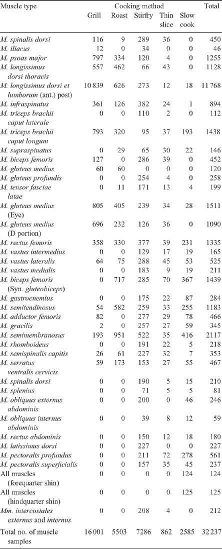
Numbers of muscle samples for each cooking method in the MSA model development database are shown in Table 1. The database, collection history and methodology were described in detail by Polkinghorne et al. (2008a). Not all cooking methods were tested on all muscles. Some high connective tissue cuts were not grilled; and most low connective tissue cuts were not slow cooked. The protocols used in testing for each cooking method are described in Gee et al. (2005) and summarised in Watson et al. (2008a). Most of the data was collected on the striploin (M. longissimus dorsi et lumborum) comprising 68% of all grilled muscles and 34% of all muscles tested by all cooking methods. This reflects the early stages of the MSA consumer testing program where the focus was on striploin testing. Also, to a lesser degree, the commercial importance of the striploin has meant that it was often the common link between experiments which involved a combination of cuts × cooking techniques. Of the five different cooking methods, grilling represented 50% of the samples tested. Stir-frying and roasting were the next most common cooking methods tested, with the thin slice method having the least number of samples tested.
|
Developing a model
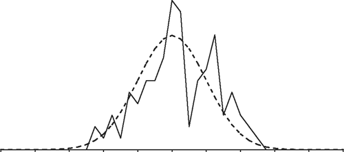
The aim of the modelling procedure was to try to find an overall smooth pattern which aligned with known meat science. To use a diagrammatic analogy: the final model was like the smooth, dotted curve shown in Fig. 1; the jagged curve relates to the effects found in the various analyses.
|
The model production process was a robust procedure in the sense that a common model was established. Effects were retained if they commonly appeared in a range of analyses at a similar level. Analyses that did not fit the common pattern were investigated to ascertain why, and included or discounted. In many cases, the questions raised by the model-fitting led to further experimentation and investigation.
Datasets analysed included the following:
-
Individual experiments;
-
Meta-analysis by combining results from individual experiments;
-
Animal effect analyses;
-
Cut-by-cut analyses; and analyses by cut groups (e.g. very high connective tissue cuts, high connective tissue cuts, low connective tissue cuts, and very low connective tissue cuts); and
-
Subsets of all of the above – both random subsets and non-random subsets (for example, categorised by variable).
Methods used included (Polkinghorne et al. 2008b):
-
Descriptive statistics – dot plots, cross-tabulations, scatter plots, etc.;
-
Regression models and general linear model fits; and
-
Validation – both statistical validation and meat scientific validation.
A commonly used tool in the model development was regression modelling, i.e. a model of the form:

The consumer variation can be averaged out (by averaging over lots of consumers). The initial intention was to try to divide the MQ formula into separate components corresponding to the meat production process:

Variables were needed to describe each of these components; and then a way found to put them together. However, these independent parts were found to be anything but independent. Furthermore, even within the parts, many of the quantities involved were interdependent.
This finding has influenced the commercial implementation of the MSA program, requiring education and reinforcement that all industry sectors interact in determining the eating quality of beef delivered to the ultimate consumer. It has also been important in dispelling various ‘silver bullet’ solutions to beef quality variously advanced and including particular breeds, attributes such as marbling or processes such as aging (Polkinghorne et al. 2008a).
Selection of variables
The 140 database columns record a large number of variables in addition to identification relating to animal groups, ear tag and slaughter body numbers and unique sample codes. These variables include breed, age and feed regime, processing inputs (including carcass suspension and electrical stimulation), conventional chiller assessment measures such as marbling, fat depth and pH, individual muscle detail (including position of the sample within muscle) and days aged. The consumer data comprised cooking method and tenderness (tn), juiciness (ju), like flavour (fl) and overall liking (ov) scores recorded in consumer testing. The MQ score was formed by weighting the four sensory scores, MQ = 0.4 × tn + 0.1 × ju + 0.2 × fl + 0.3 × ov, obtained using optimum linear discriminating function (Watson et al. 2008a). The model development process, as discussed in the following sections, sought to identify and quantify variables, which assisted in describing the consumer tested outcomes.
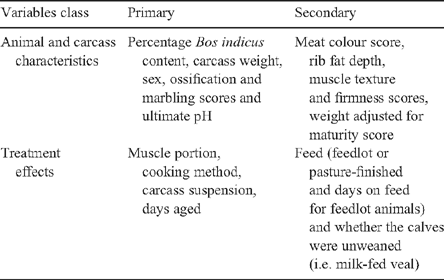
Variables which consistently added to predictive ability were retained in the model whereas those which demonstrated no relationship, or were inconsistent, were discarded. An example of this were texture and firmness scores, which despite repeated analysis, failed to predict eating quality either as single variables, or in combination with others. In some instances, a selection needed to be made between alternative variables which essentially described different aspects of the same characteristic in the carcass. Examples of this were the different measures for fatness which generally were positively correlated within any of the datasets, e.g. P8 and rib fat depths and USDA and AUS-MEAT marbling scores were all positively correlated. In cases like this, trade-offs between reliability, availability, sensibility and transparency had to be made. After considerable discussion, statistical input and debate, the variables presented in Table 2 were considered as candidates for modelling.
|
The primary variables were included as they all had significant predictive value for MQ; whereas the secondary variables were subject to further investigation. Ultimately, the feed variables (such as feed, days on feed) were deleted as the effect of feedlotting on palatability was found to be adequately covered by carcass weight, ossification and marbling score effects. The further addition of feed or days on feed was found to have little consistent additional effect.
The weight adjusted for maturity score variable was calculated as a ratio of estimated liveweight (i.e. carcass weight/0.56) relative to age (estimated by ossification score) in an attempt to describe the lifetime growth rate of the animal. However, as reported by Thompson et al. (1999), the use of this ratio to predict the MQ score had some statistical complications. Examination of the interaction between ossification score and carcass weight was found to provide a better model to describe the relationships with the MQ score. A gradual change in the slope of carcass weight to the MQ score, within ossification score provided a model which allowed a meat science interpretation to be proposed.
Although the effect of ultimate pH (pHu) below 5.7 on the MQ score was found to be minimal, pHu was retained as a predictor variable as it was the basis of a cut-off criterion. In the presence of pHu both AUS-MEAT and USDA meat colour scores added little to the prediction of the MQ score. Rib fat was also used as a censoring variable, but since it was found to have some impact for several muscle portions it was retained in the model in preference to other fat measures.
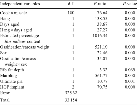
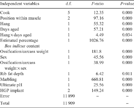
To indicate some of the effects of the model, an ANOVA is presented in Table 3. The model fitted for the common ANOVA is as follows:
|

where cook is cooking method, hang is tenderstretch or Achilles hung, dagd is days aged post-mortem, osswt is ossification carcass weight score, sex is heifer or steer, umb is USDA marbling score, rbf is rib fat depth and hgp is hormonal growth implant indicator. In this model, ‘hang|dagd’ represents hang effect + aging effect + hang × aging interaction, which indicates the difference in aging effect for different methods of hanging. Similarly, for ‘osswt|sex’ represents osswt + sex + osswt × sex. The latter term indicates the difference in the carcass weight/ossification effects between males and females. The estimated percentage Bos indicus content was represented by epbi and treatment using hormone growth promotant implants by HGP.
This ANOVA is too simple in the sense that it does not allow for a range of effects. Essentially, everything interacts with cook × muscle; and there are interactions between several of the other variables, which are also ignored in this analysis. However, it provides an indication that each of these variables had some effect.
This model also ignored animal effects; as do most of the model analyses: the model was intended to replace the animal effects by observable variables such as epbi, ossification score, carcass weight, sex, rib fat depth, marbling and so on, which can be used for prediction. In most instances, when the model is fitted, it is fitted for each cut separately, so that there is generally only one cut from each animal included in such an analysis.
The ANOVA obtained for the striploin (M. longissimus dorsi et lumborum) data is given in Table 4.
|
Again, each of the parameters is shown to have some effect indicating the significant variation found within this muscle. The striploin has been used extensively in beef research and there are many reports of variation and sensitivity to animal and processing effects (e.g. Dransfield 1977; Shorthose and Harris 1990; Shackelford et al. 1995). The appropriateness of using the striploin as an indicator cut for other carcass muscles has also been discussed and challenged by Shorthose (1996) who suggested the eye round (M. semitendinosus) as an alternative less subject to processing variation. Koohmaraie et al. (1998) and Rhee et al. (2004) also found the correlation between meat quality measurements (both sensory and objective) for the striploin and other muscles in the carcass to be weak.
ANOVA for each individual muscle (data not shown) produced varying rankings of importance, as measured by F-ratios, for the principal variables further indicating that the palatability of each muscle would be best estimated individually rather than from a common indicator muscle. This presented a challenge to the traditional approach of grading a carcass as a unit v. its individual muscles. Polkinghorne (2005) used the MSA model prediction of palatability for a range of muscles from carcasses from different production systems subjected to a range of processing conditions. Polkinghorne concluded that it is not possible to provide meaningful estimates of palatability for a range of cuts from a simple striploin relationship.
Input variable analysis
Epbi
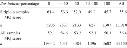
The epbi is among the most consistent animal-based indicators identified in the modelling process, appearing as significant in most analyses. Table 5 gives the raw mean MQ score by epbi split into five categories; for striploin data, and for all data. This table is simply an indicator of the negative relationship that exists between consumer scores and the epbi. Clearly, many other factors are involved. Here it is assumed that with the large numbers of samples involved the other factors are averaging out. Negative eating quality effects with Bos indicus cattle have also been widely reported by others including Koch et al. (1976), Sherbeck et al. (1996) and Koohmaraie et al. (1998).
|
Epbi relationship to carcass hump height
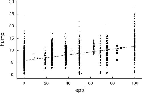
The epbi of research cattle groups was known, but for commercial cattle, the epbi was based on the producer’s report. As grading results and producer payment were related to the epbi declared it was also felt there could be some uncertainty in its veracity. Furthermore, in some cases, an average value for a group of cattle was given, and there was clear variation within the group. A check was devised to provide an objective assessment by considering the carcass hump height in relation to carcass weight. The relationship between carcass hump height and epbi is indicated in Fig. 2.
|
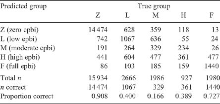
A discriminant analysis for the epbi (categorised into five groups) on hump height and carcass weight yielded the best discriminant function: hump (mm) – 0.1 × carcass weight (kg). With this discriminator the results presented in Table 6 were obtained.
|
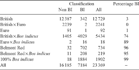
The percentage Bos indicus group cut-offs used in the analysis above were 37, 52, 60 and 84. Using hwd <40 as the epbi = 0 indicator (to be conservative and reduce the risk of misclassifying too many Bos taurus animals), the results presented in Table 7 were produced from a comparison of the proposed hump-based Bos indicus estimate in relation to breed type as recorded in the dataset.
|
Apart from the Belmont Reds, very few zero (reported) epbi were misclassified and most of any part Bos indicus animals were correctly classified. The hump-estimated percentage Bos indicus adjustment upgraded epbi to a higher level if hump was significantly greater than the equivalent for the reported epbi.
As a result of this analysis, a hump and carcass weight-based adjustment was incorporated into the model. Carcasses which fell outside the established relationship were reassigned to a more appropriate percentage Bos indicus level. In addition to providing a cross check against the declared epbi of carcasses presented for grading, this also provided a means to grade carcasses on-line without a producer declaration. While there is some risk that the calculated epbi may be greater than the true percentage, this procedure can be commercially useful where slaughter groups vary widely in epbi. The alternative was to draft animals into epbi categories before slaughter, which would have generally subjected the animals to stress before trucking or lairage and, therefore, potentially reduced glycogen content.
The above adjustment based on hump height and carcass weight, rated Belmont Reds, a tropically adapted Bos taurus and Africander-derived breed, as if they were part Bos indicus. An analysis of the Belmont Red animals indicated that their meat palatability rated close to that of animals with epbi = 50. In other words, they were similar to 50% epbi animals, in palatability as well as in their hump height. This was generally consistent with relationships of tenderness in Brahman-based cattle to phenotype reported by Sherbeck et al. (1996). Thus, a further adjustment to the epbi conversion for Belmont Reds was not required.
Ossification score and carcass weight
Ossification is an assessment of the calcification of the cartilage in the sacral and dorsal vertebrae. Other workers have examined the relationship between tenderness and skeletal maturity scores with some studies showing a negative relationship between maturity and tenderness scores (Smith et al. 1982, 1988; Hilton et al. 1998; Park et al. 2008), whereas others have failed to find any relationship (Romans et al. 1965; Carroll et al. 1976; Field et al. 1997). The USDA grading system utilises ossification score in conjunction with meat colour to create a maturity score, which is in turn associated with marbling to assign a quality grade. It was identified as a potential modelling input due to its USDA system inclusion, so carcass ossification was recorded from the first MSA trials. The score assigned by MSA graders is a numeric presentation of the USDA scale in increments of 10 where A0 = 100, B0 = 200, C0 = 300 out to E90 = 590 (Romans et al. 1965).
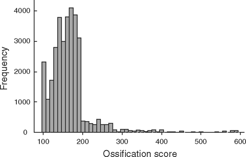
Figure 3 presents the distribution of ossification values in the model development dataset. The majority of the data are in the 100–200 ossification range. The early MSA pathways and initial models limited ossification to a maximum of 200, reflecting opinion from the USDA B0 cut-off, and there was a lack of data beyond this threshold: the early testing was primarily of young cattle destined for the Australian domestic market. Although this constraint was subsequently removed, the skewed distribution is a legacy of the earlier grading constraints.
|
A majority of the 100 ossification scores relate to cuts derived from milk-fed vealers (i.e. they were unweaned calves still suckling the cow when transported for slaughter and coded MFV in the database). While the data encompassed a considerable range in ossification score, this number varied by muscle. There were far fewer samples with high ossification scores and for some muscles there were very few ossification scores at the high end of the range. MSA is testing further samples with high ossification scores in order to better support the model for ossification scores greater than 300.
The dataset shows a general downward effect on the MQ score with increasing ossification score, and this is especially evident with lower ossification scores. As expected, younger animals tend to be associated with higher MQ scores.
Modelling carcass weight is not so straightforward. Ignoring other factors, the regression of MQ score on weight is curvilinear. The MQ score is high when it is small and when the weight is large, with a minimum at around 300 kg.
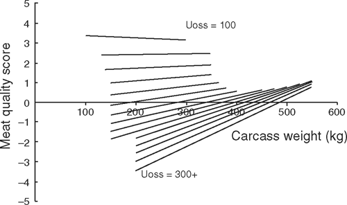
The following ossification/carcass weight model allowed a differential effect of carcass weight within each ossification score category subject to the criteria that: ‘MQ increased with carcass weight within each ossification category’ and ‘for any given carcass weight, the lower ossification score (younger animal) was more palatable’. The relationships between carcass weight and palatability within ossification score category were assumed to be linear and are shown in Fig. 4. At low ossification scores the slope between carcass weight and palatability was close to zero, but it increased gradually as the ossification scores increased.
|
This model was fitted by using a weighted average of the separate fits for each of the muscles. For many of the muscles in which there were reasonable numbers of observations and a wide range in ossification score (e.g. the striploin) the result needed some adjustment to ensure that the slopes of the lines were not negative and did not intersect within the range of likely carcass weights. Although all slopes were positive, the fitted line for ossification score 100 had a slightly negative gradient. This was retained in the model as it was felt that, for this ossification category, smaller weight may reflect lesser age and, therefore, for the MFV, may be associated with increased palatability.
For muscles in which the datasets were more sparse, the intercept and slope values for carcass weight within ossification score were erratic. However, even with these reduced datasets, the same general trends were evident. Instead of fitting ossification score as a fixed effect in the interaction with carcass weight, it was fitted as a covariate to obtain a smoothed function for the slope and intercept for different muscles. The variability of the coefficients for the muscle × ossification/carcass weight interaction was modelled as follows:

where g(oss,cwt) denotes the ossification/carcass weight score defined by Fig. 4, and the multiplier k (muscle) is allowed to vary from muscle to muscle. If the ossification/carcass weight is important for a muscle then k (muscle) is large, but if it is not important then k (muscle) is small: the average of the k-values was around 1. Again, the results appear to have a plausible meat science interpretation in that high k-values tend to occur for high activity and connective tissue muscles. For the ossification categories for which there were MFV animals (i.e. ossification score ≤140) there was an additional positive MFV effect of 4 MQ points on average.
Carcass suspension and aging
Carcass suspension and aging effects are discussed together due to their interaction, as highlighted by early analysis of the MSA database. This substantially increased the sample collection program as data for each carcass suspension method needed to be over a range of days aged for each of the muscles examined.
Carcass suspension
The model development database contained palatability results from several carcass suspension treatments. These included carcasses suspended by the Achilles tendon (AT), suspended from the obturator foramen (TX), suspended from the sacral ligament (TL) and carcasses which were prepared using the tendercut procedure (TC) described by Wang et al. (1994).
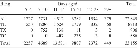
The majority (68%) of the dataset were AT hung, with a substantial minority (27%) TL hung, with relatively few TX and TC samples (3 and 2%, respectively), and not enough to allow incorporation of these methods in the model (Table 8). Work continues to extend the modelling range for the TX method.
|
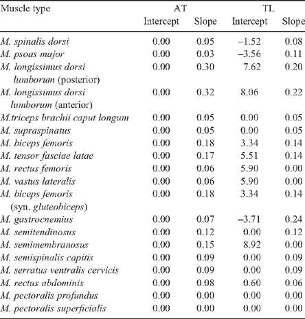
Not surprisingly, it is found that the effect of carcass suspension method on palatability (MQ score) interacted with muscle. The effect of the TL carcass suspension method (at 5 days aging) is indicated in Table 9 by the TL intercept column, with the AT intercept column set to zero. The MQ score of M. longissimus dorsi lumborum, M. biceps femoris and M. semimembranosus were improved by the TL hanging method, while the M. psoas major and M. spinalis dorsi were negatively affected. In general, forequarter cuts tend not to be affected by the TL method compared with the AT method.
|
Hwang et al. (2002) compared the TX and TL carcass suspension methods against AT using consumer taste panels to evaluate stir-fry samples from 18 hindquarter muscle/muscle portions at 10 days aging. They showed that both tenderstretch (TL and TX) methods resulted in an improvement in hindquarter and loin muscles relative to AT hanging.
The limited TC data was obtained from three separate experiments utilising cattle from three abattoirs. The cattle included unweaned 10-month-old British breed steers, ~30-month-old British breed steers and ~30-month-old British breed, Bos indicus and Piedmontese cross steers. Tenderstretch and Achilles comparisons were made within each group with from 9 to 13 muscles tested under grill, roast and slow cooking methods.
Post-mortem muscle aging period
At an industry level, aging was generally believed to improve eating quality but knowledge of the degree and rate of improvement or of differences between muscles was limited at best. Differences in the aging potential of various muscles have been reported by Bouton and Harris (1972), Dransfield (1994) and others. Bouton and Harris (1972) also reported differences in aging rate between muscles and between the same muscles under different suspension treatments; and further, they reported a decline in aging rate over time. The potential for differential aging effects between muscles and suspension methods dictated a need for considerable data to develop plausible estimates for modelling.
The number of samples available in the model development dataset by aging period, muscle and hanging method is presented in Table 8. All aging was conducted at 1–4°C in a vacuum pack. Initially, the entire primal was aged, whereas later samples were fabricated from the primal and re-vacuumed before freezing at the designated aging days.
While this is a large dataset, the numbers in individual (muscle × days aged × hanging method) cells were often small. All samples were aged for a minimum of 5 days, which was set as an MSA requirement. The majority of the aging data were in the range 7–21 days, with most in the 11–14 days category. There was very little information beyond 28 days aging, resulting in the model predictions being restricted to a 28-day maximum.
In general, aging tends to even things out: when the meat palatability improves with age, it improves at a faster rate for the hanging method that is behind at 5 days. However, within the range of the available data, it never catches up.
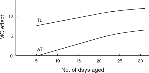
A common result for the effect of days aged on MQ is shown in Fig. 5, for the posterior striploin. Striploins from TL carcasses were substantially more palatable at 5 days than those from AT carcasses. However, the difference reduced with aging time at least up to ~25 days.
|
The three experiments conducted to compare hanging methods TL, AT and TX included 13 muscles derived from a range of cattle types sourced from different abattoirs. While this generated a useful dataset, all carcass muscles were not tested and aging comparisons were limited to a range of 13–20 days. Therefore, it was not possible to independently derive the coefficients for all the muscle × aging combinations. However, the available data show that the TC option is between the AT and the TL method in terms of the effects on palatability of the hindquarter muscles. Figure 5 presents the hang × age effect estimated for the AT and TL striploin data.
Aging effects were derived for all muscle × hang combinations in the dataset, although the available data restricted the reliability for some cells. The fitted effect for each was obtained as a straight line. The value used in the model, for each hang method × muscle, was assumed to be linear up to days aged = 20. The literature would suggest a declining rate of increase in eating quality with aging, so an exponential curve was used for aging times greater than day 20, reflecting caution with prediction for higher aging times by ensuring that no matter what value for days aged was used the benefit could never exceed the fitted linear value at 30 days.
Marbling and fat: umb, amb, rbf, P8
The umb and amb (AUS-MEAT marbling score) are assessments of marbling. In addition rib fat depth (mm) at the quartering point and P8 fat depth (mm) are measurements of carcass fatness, primarily of the subcutaneous fat depot. The range of values, the slightly higher correlation with MQ, and ultimately the predictive value in concert with other model variables led to the choice of umb and rbf as grading model inputs.
The variable umb came to take on the role of a surrogate for at least part of the effects of several other variables and so, with this in mind, it is not that surprising that it appears consistently in the prediction model for all cuts, although with varying relative importance to other input variables.
Rib fat has less effect on the model; but, like pHu, it has a censoring role. Animals with rbf less than 3 mm are rejected. The reasoning for including a minimum rib fat requirement relates to even chilling within the muscle (Polkinghorne et al. 2008a).
HGP implants
Initially, HGP use was not recorded in the database. After several years of data collection it was thought appropriate to add it to the list of variables and, where possible, it was added retrospectively.
The dataset relating to HGP was further boosted by data from several trials conducted to investigate HGP effects on eating quality. The use of HGPs has been studied extensively in the database (Thompson et al. 2008a; Watson 2008; Watson et al. 2008b), and in a range of associated experiments reported elsewhere. The result was an HGP penalty of the order of 3–6 MQ points on meat palatability, depending on the muscle which is further adjusted with aging.
The process of combining the results from several independent HGP experiments and deriving a final application for use in the grading model is further discussed by R. Polkinghorne, J. Thompson and R. Watson, unpubl. data.
Other variables considered for inclusion in the model
In addition to the primary variables selected for use within the prediction model, several others were evaluated at various points. These are briefly discussed below.
Feedlot variables: finishing system and days on feed
Finishing system indicated whether the animals had been finished on a high grain ration or on pasture. Within feedlot finish, the days on feed were also recorded. Both these variables were eventually omitted from the model as variance explained by finishing system was similar to that explained by the increased carcass weight relative to ossification and higher marbling scores associated with feedlot finishing systems. It seemed preferable to model using an outcome variable (carcass weight, ossification and marbling) rather than a treatment variable (feed) and so both finishing system and days on feed were excluded from the model.
pHu, AUS-MEAT meat colour and USDA colour of lean scores
Several attempts were made to incorporate pHu or a colour variable into the model. However, any such effects seemed always to be driven by the extreme values, which would be culled in practice anyway. It was decided to effectively leave these variables out of the model, except in their role as censoring variables and as a minor effect in the case of pHu. If the pH or the colour was too extreme, then the meat was discarded. Any carcass with a pHu beyond 5.7 or an AUS-MEAT meat colour above 3 is excluded from grading.
Establishment of a base cut × cook relationship
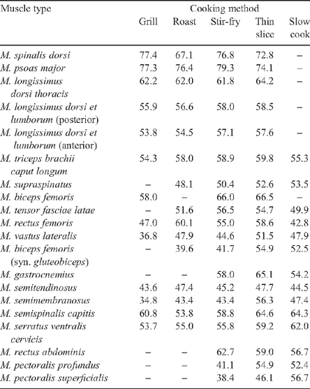
As the core retained variables were identified from muscle by muscle and overall analysis a base muscle × cook table of MQ scores was constructed (Table 10). Essentially, this comprised the data means.
|
In fitting the model based on the variables described in the previous section, it was decided to treat as baseline the ‘standard’ case given by:

Table 10 specifies the model ‘intercept’, i.e. the predicted value with all the variables set at baseline level. Thus, these can be interpreted as the predicted values for the standard animal/treatment.
In applying the model, the predicted values for each muscle × cook combination are calculated as deviations from these standard scores, depending on the deviations of each of the predictor variables from their standard values, specified in Table 10.
Accuracy of the prediction model
An indication of the accuracy of the prediction model was given by applying it to the MSA dataset. For each meat sample, the observed MQ value was compared with the predicted MQ. This was applied to every sample for which a prediction was possible, even those with incomplete or doubtful data, or input values that would have excluded them from the grading process. The results are indicated in Table 11. In most cases, the average difference was less than 1 and in only 5/72 (7%) of the cells does a simple t-test indicate a non-zero mean at the 5% level.
Analysis indicates that the standard error for most of the predicted MQ scores will be less than 1. But these standard errors are based on the assumption that the model is correct, and so must be treated with some caution. It does suggest that, if the model is close to the truth, then the predicted mean scores will mostly be within 2 units of the population mean MQ score. However, predicting a mean MQ is different from predicting where the actual consumers’ MQ scores will be: i.e. actual MQ scores will be distributed around this mean with a standard deviation of the order of 8–10.
The results in Table 11 are consistent with the accuracy of the MSA model presented by Thompson (2002). In his analysis, Thompson (2002) calculated whether the consumer grade in terms of eating quality aligned with the grade assigned by the model. It was shown that the accuracy of the model was of the order of 50–70% and, if there were deviations between the assigned and allocated grades, the deviation was only of the order of one grade.
Based on an independent dataset of three muscles which had been taste-tested by Australian and Korean consumers, Thompson et al. (2008b) showed that accuracy of grade allocation was of the order of 59 and 53% for Korean and Australian consumers, respectively. When the data were examined, on the basis of residuals, the deviations were similar to those reported in this study, with the exception of the M. semimembranosus where deviations were of the order of 2–8 points on the MQ scale.
Model output for commercial application
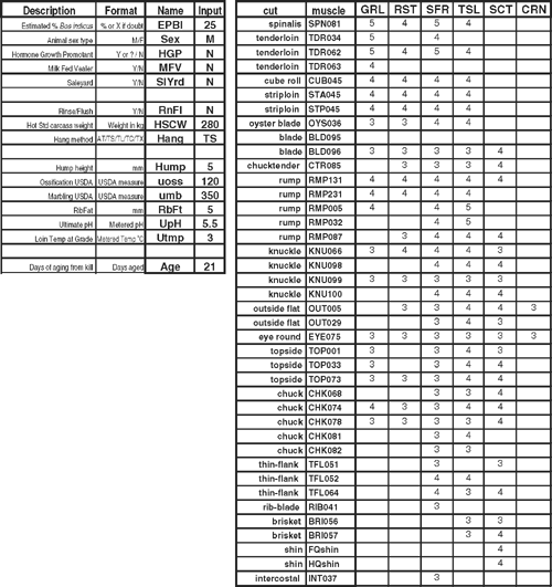
While the primary use of the prediction model is as a grading tool, it is also an integral part of the extension and education efforts of explaining the basis of the MSA system to industry and in demonstrating the predicted eating quality impact of changes to the various input variables. Figure 6 presents a diagrammatic representation of the model predictions for a sample carcass. The input variables are displayed to the left hand top corner. The predicted grade for each muscle × cooking combination at the specified days aged is shown in the right hand portion. The grades displayed are determined from an individual MQ points score for each of the cut × cook combinations.
|
While this form of display is used to demonstrate the model the relevant information is transferred as a data string in commercial grading applications. The data are transferred from the hand-held data capture unit (DCU) and can be uploaded to abattoir management information systems to produce mandatory feedback reporting to suppliers and can be integrated with traceability and management systems to allow eating quality scores to be modified with aging and tracked through inventory. Under current commercial practice, carcasses are most commonly assigned to stratification groups at the point of grading. Stratification groups, based on minimum MQ grade scores for any nominated cuts at specific days aged for specified cooking methods, are defined by the abattoir. The DCU is programmed to check each carcass against the stratification specification and allocate appropriately. This allows carcasses to be marshalled into runs for fabrication. Further discussion of commercial application of the model output is provided by Polkinghorne et al. (2008a).
Conclusions
This paper describes the statistical development of the MSA prediction model for beef palatability. This model is essentially a descriptive model, with the intention of describing the large amounts of data collected by MSA. The model is constrained to accord with accepted meat science principles and smoothness.
A broad range of input variables as discussed above are applied interactively on a muscle by muscle basis to produce a predicted consumer score for each muscle × cooking method combination. This score is used to allocate cuts into three consumer defined acceptable quality grades or an unsatisfactory ungraded category. This prediction for individual muscles is a significant advance from applying a single quality grade to an entire carcass as a basis for grading.
Although we have derived a plausible and smooth model that described the available data well, this is not to say that the dataset could not be described at least as well by some other model. But what is true is that the model does provide a reasonable description of the data, which does appear to be useful in prediction. The words of George Box, Statistician, should be kept in mind here: ‘All models are wrong … but some are useful’ (Box and Draper 1987, p. 424).
Also worth repeating is the point that the model has been developed for active commercial use. While developed from a large number of controlled experiments and additional less controlled commercial collections the average performance of the model over a full range of commercial environments must take precedence to its accuracy on any specific set of experimental data. Additional data and ongoing analysis will enable further improvement and new versions are planned to maintain currency with consumer preference, which may change over time, and to make full use of additional data and analysis.
Bouton PE, Harris PV
(1972) The effects of some post-slaughter treatments on the mechanical properties of bovine and ovine muscle. Journal of Food Science 37, 539–543.
| Crossref | GoogleScholarGoogle Scholar |

Carroll FD,
Ellis KW,
Lang MM, Noyes EV
(1976) Influence of carcass maturity on the palatability of beef. Journal of Animal Science 43(2), 413–417.

Dransfield E
(1977) Intramuscular composition and texture of beef muscles. Journal of the Science of Food and Agriculture 28, 833–842.
| Crossref | GoogleScholarGoogle Scholar |
CAS |

Dransfield E
(1994) Optimisation of tenderisation, ageing and tenderness. Meat Science 36, 105–121.
| Crossref | GoogleScholarGoogle Scholar |

Field R,
McCormick IR,
Balasubramanian V,
Sanson D,
Wise J,
Hixon D,
Riley M, Russell W
(1997) Tenderness variation among loin steaks from A and C maturity carcasses of heifers similar in chronological age. Journal of Animal Science 75, 693–699.
|
CAS |
PubMed |

Hilton GG,
Tatum JD,
Williams SE,
Belk KE,
Williams FL,
Wise JW, Smith GC
(1998) An evaluation of current and alternative systems for grading quality carcasses of mature slaughter cows. Journal of Animal Science 76, 2094–2103.
|
CAS |
PubMed |

Kim CJ, Lee ES
(2003) Effects of quality grade on the chemical, physical and sensory characteristics of Hanwoo (Korean native cattle) beef. Meat Science 63, 397–405.
| Crossref | GoogleScholarGoogle Scholar |

Koch RM,
Dikeman ME,
Allen DM,
May M,
Crouse JD, Campion DR
(1976) Characterization of biological types of cattle. III. Carcass composition, quality and palatability. Journal of Animal Science 43, 48.

Park BY,
Hwang IH,
Cho SH,
Yoo YM,
Kim JH,
Lee JM,
Polkinghorne R, Thompson JM
(2008) Effect of carcass suspension and cooking method on the palatability of three beef muscles as assessed by Korean and Australian consumers. Australian Journal of Experimental Agriculture 48, 1396–1404.

Polkinghorne R,
Philpott J,
Gee A,
Doljanin A, Innes J
(2008a) Development of a commercial system to apply the Meat Standards Australia grading model to optimise the return on eating quality in a beef supply chain. Australian Journal of Experimental Agriculture 48, 1451–1458.

Polkinghorne R,
Thompson JM,
Watson R,
Gee A, Porter M
(2008b) Evolution of the Meat Standards Australia (MSA) beef grading system. Australian Journal of Experimental Agriculture 48, 1351–1359.

Rhee MS,
Wheeler TL,
Shackelford TL, Koohmaraie M
(2004) Variation in palatability and biochemical traits within and among eleven beef muscles. Journal of Animal Science 82, 534–550.
|
CAS |
PubMed |

Romans JR,
Tuma HJ, Tucker WL
(1965) Influence of carcass maturity and marbling on the physical and chemical characteristics of beed. 1. Palatability, fiber diameter and proximate analysis. Journal of Animal Science 24, 681.
|
CAS |
PubMed |

Shackelford SD,
Wheeler TL, Koohmaraie M
(1995) Relationship between shear force and trained sensory panel tenderness ratings of 10 major muscles from Bos indicus and Bos taurus cattle. Journal of Animal Science 73, 3333–3340.
|
CAS |
PubMed |

Sherbeck JA,
Tatum JD,
Field TG,
Morgan JB, Smith GC
(1996) Effect of phenotypic expression of Brahman breeding on marbling and tenderness traits. Journal of Animal Science 74, 304–309.
|
CAS |
PubMed |

Shorthose WR
(1996) A qualitative model of factors influencing beef tenderness. Proceedings of the Australian Society of Animal Protection 21, 143.

Shorthose WR, Harris PV
(1990) Effect of animal age on the tenderness of selected beef muscles. Journal of Food Science 55, 1–8, 14.
| Crossref | GoogleScholarGoogle Scholar |

Smith GC,
Cross HR,
Carpenter ZL,
Murphey CE,
Savell JW,
Abraham HC, Davis GW
(1982) Relationship of USDA maturity groups to palatability of cooked beef. Journal of Food Science 47, 1100–1107, 1118.
| Crossref | GoogleScholarGoogle Scholar |

Smith GC,
Berry BW,
Savell JW, Cross HR
(1988) USDA maturity indices and palatability of beef rib steaks. Journal of Food Quality 11, 1–13.
| Crossref | GoogleScholarGoogle Scholar |

Thompson JM
(2002) Managing meat tenderness. Meat Science 62, 295–308.
| Crossref | GoogleScholarGoogle Scholar |

Thompson JM,
McIntyre BM,
Tudor GD,
Pethick DW,
Polkinghorne R, Watson R
(2008a) Effects of hormonal growth promotants (HGP) on growth, carcass characteristics, the palatability of different muscles in the beef carcass and their interaction with aging. Australian Journal of Experimental Agriculture 48, 1405–1414.
|
CAS |

Thompson JM,
Polkinghorne R,
Hwang IH,
Gee AM,
Cho SH,
Park BY, Lee JM
(2008b) Beef quality grades as determined by Korean and Australian consumers. Australian Journal of Experimental Agriculture 48, 1380–1386.

Thompson JM,
Polkinghorne R,
Porter M,
Burrow HM,
Hunter RA,
McCrabb GJ, Watson R
(2008c) Effect of repeated implants of oestradiol-17β on beef palatability in Brahman and Brahman cross steers finished to different market end points. Australian Journal of Experimental Agriculture 48, 1434–1441.
|
CAS |

Wang H,
Claus JR, Marriott NG
(1994) Selected skeletal alterations to improve tenderness of beef round muscles. Journal of Muscle Foods 5, 137–147.
| Crossref | GoogleScholarGoogle Scholar |

Watson R
(2008) Meta-analysis of the published effects of HGP use on beef palatability in steers as measured by objective and sensory testing. Australian Journal of Experimental Agriculture 48, 1425–1433.
|
CAS |

Watson R,
Gee A,
Polkinghorne R, Porter M
(2008a) Consumer assessment of eating quality – development of protocols for Meat Standards Australia (MSA) testing. Australian Journal of Experimental Agriculture 48, 1360–1367.

Watson R,
Polkinghorne R,
Gee A,
Porter M,
Thompson JM,
Ferguson D,
Pethick D, McIntyre B
(2008b) Effect of hormonal growth promotants on palatability and carcass traits of various muscles from steer and heifer carcasses from a Bos indicus–Bos taurus composite cross. Australian Journal of Experimental Agriculture 48, 1415–1424.
|
CAS |


