

GPS tracking informs nest reserve design for an endangered raptor, the grey goshawk (Tachyspiza novaehollandiae), in hostile anthropogenic landscapes
David A. Young A * and James B. Kirkpatrick A †
A
† Deceased, October 2024. Responsible for Methodology and Supervision.
Handling Editor: Laura Wilson
Abstract
We used GPS telemetry to investigate space use and movements of 15 grey goshawks (Tachyspiza novaehollandiae) in south-east Tasmania, Australia, between 2021 and 2023. The number of nests per territory in 73 active breeding territories was also determined and inter-nest distances were calculated. Mean minimum convex polygon (MCP) non-breeding season home range size of female goshawks was more than twice as large as the mean breeding season home range size. Home range size of males was similar in the breeding and non-breeding seasons and the MCP estimates suggest their home ranges are much larger than that of females. Tracked goshawks were range residents throughout the year with kernel density (KD) core areas centred on nest trees and preferred foraging locations. Movement patterns were highly recursive although some individuals occasionally undertook long range excursions away from their nests. Mean number of nests per goshawk breeding territory was 2.0 (range 1–6). Median distance between nests in breeding territories was 78.0 m (range 1.8–915.0 m). We recommend that prescriptive nest reserves for grey goshawks be implemented based on our 50%, 75% and 95% KD core area estimates for females in the breeding season. We provide a conceptualised example of a nest reserve design.
Keywords: endangered raptor, goshawk, GPS, home range, kernel density, nest reserve.
Introduction
Knowledge of space use, movements and breeding ecology is critical for species conservation (Cadahía et al. 2007; Bosch et al. 2010; van Eeden et al. 2017; Mancinelli et al. 2018). Estimates of home range metrics (i.e. size, shape, core areas) and movement patterns can be used to identify specific areas or important habitats to target for conservation, reservation status or increased management attention (Reynolds et al. 1992; Kennedy and Andersen 1999; Boal et al. 2001; McLeod et al. 2002). These data also allow decision makers or planners to visualise and comprehend the most appropriate spatial scales at which to implement conservation strategies (Dick and Plumpton 1999; Coast Forest Conservation Initiative (CFCI) 2012). Developing a reliable and statistically robust metric consistent across individuals, species and habitats is important (Jacobson et al. 2024). However, such information is usually lacking for threatened or declining species, as they are often rare or challenging to study due to low breeding densities, cryptic behaviour, or they occupy hostile environments (Andersen et al. 2004; Cadahía et al. 2005; Robillard et al. 2018). For example, species that occur in remote and inhospitable areas (i.e. polar regions or deserts) or those with restricted or broad distributions (i.e. habitat specialists and migratory species) are usually data deficient (Butchart and Bird 2010; Therrien et al. 2011; Wiig et al. 2015).
Although estimates of overall home range size are informative and useful for wildlife management, estimating core areas (i.e. breeding locations) based on recursive movements is of greater importance for the conservation of at-risk species, particularly raptorial birds as they are central place foragers when breeding (Orians and Pearson 1979; Bright-Smith and Mannan 1994; McPherson et al. 2019). In recent decades, GPS tracking technology has revolutionised the acquisition of spatial data to perform such tasks (Prince et al. 1992; Cadahía et al. 2007; Blakey et al. 2020; Murgatroyd et al. 2023). GPS telemetry has also played a key role in determining seasonal migration routes (Limiñana et al. 2012), resource selection (Moser and Garton 2019) and ranging behaviour (Garcia-Ripolles et al. 2011) of threatened or data deficient raptors. GPS telemetry is also commonly used now as a risk assessment tool for raptors, especially for the renewable energy and resource extraction sectors (Vignali et al. 2022; Boggie et al. 2023). For example, collision risk modelling (CRM) is routinely undertaken for eagle species and other birds, based on GPS tracking data of flight behaviours, to inform the design and spatial layout of wind farm turbines to minimise collision risk and associated mortalities (May et al. 2011; Murgatroyd et al. 2021).
Describing space use of raptors from GPS telemetry data is increasingly performed with density-based estimators such as kernel density (KD), and brownian bridge movement models (BBMM), in addition to minimum convex polygon or convex hull methods (MCP and CH) (Kie et al. 2010; Kranstauber et al. 2012; McPherson et al. 2019). Density based methods are considered to be superior for conservation management purposes because they identify the location of core areas and provide important quantitative data on relative use of specific areas (i.e. defended territories) or habitats within the home range based on utilisation distributions (UD) and occurrence probabilities (Worton 1989; Seaman and Powell 1996; Horne et al. 2007). Core area metrics and features (i.e. the location, habitats, size) are often used as ‘primary input data’ to inform the design of breeding habitat reservations or core nest reserves for threatened or declining species (Reynolds et al. 1992; Youtz et al. 2008; Bilney et al. 2011; Coast Forest Conservation Initiative (CFCI) 2012).
We studied space use, movements and nesting ecology of the grey goshawk (Tachyspiza novaehollandiae; Gmelin, JF, 1788; Kaup 1844), a medium sized raptor that breeds in wet forests throughout the island state of Tasmania, Australia. The species occurs at low densities throughout its range but can be locally common in well forested, agricultural landscapes. It is currently listed as endangered under Tasmania’s Threatened Species Protection Act 1995 due to its small population size, restricted breeding distribution and ongoing habitat loss (Forest Practices Authority 2002; Threatened Species Section 2022). Other potential threats include persecution, disturbance at nest sites, electrocution from electricity infrastructure, collisions with vehicles, anti-coagulant rodenticides and bioaccumulation of toxic chemicals (Threatened Species Section 2022). Mooney and Holdsworth (1988) estimated the population to be 70–110 breeding pairs; however, the current status is unknown. Although it is listed as endangered under state legislation in Tasmania, it is not listed under the Commonwealth’s Environment Protection and Biodiversity Conservation Act 1999 (EPBC Act 1999) as the Tasmanian population is currently not considered to be a subspecies.
The grey goshawk is widely distributed in Australia, from the Kimberley (WA) region in the north-west, through the north, down the entire east coast into Victoria and across Bass Strait into the island state of Tasmania, where only the white morph occurs (del Hoyo et al. 2014; BirdLife International 2016). They are forest habitat generalists using a variety of forest types and habitats for foraging (Olsen et al. 1990; Burton and Olsen 1997). They prey on small native mammals and birds primarily, although introduced species are common prey items in anthropogenic landscapes (Mooney and Holdsworth 1988; Olsen et al. 1990). Breeding adults appear to be territorial, range residents in Tasmania, with breeding taking place in spring/summer between mid-September and February (Brereton and Mooney 1994; D. Young, S. Harwin, J. B. Kirkpatrick, unpubl. data). Previous studies suggest they prefer to nest in mature, wet forests and breeding pairs have several nests within a territory (Brereton and Mooney 1994; Forest Practices Authority 2010; Tierney 2011; Young and Kirkpatrick 2024; D. Young, S. Harwin, J. B. Kirkpatrick, unpubl. data). Young and Kirkpatrick (2024) reported an average inter-nest distance of 2.4 km between neighbouring pairs, which suggests home range sizes are probably around 1800–3000 ha. A study by Burton and Olsen (2000) on the species in Queensland reported (MCP) home range sizes of 80 ha for males and 11 ha for females in the breeding season, and 105 ha for males and 587 ha for females in the non-breeding season, based on radio-telemetry data. However, no published studies have used GPS telemetry to estimate home range size and core areas in Australia.
The aim of this study is to investigate space use, movements and nesting ecology of GPS tracked grey goshawks in modified landscapes of south-east Tasmania, Australia. The main objectives were: (1) estimate overall home range size (i.e. the habitat extent – 100% MCP) of adult goshawks during the breeding and non-breeding seasons, (2) identify and quantify the size of core areas (50%, 75% and 95% isopleths) using kernel density (KD) estimation, (3) determine the number of nests in goshawk breeding territories and calculate within territory, inter-nest distances, (4) use KD estimates to inform nest reserve design and (5) provide a conceptualised example of a nest reserve design.
Materials and methods
Study area
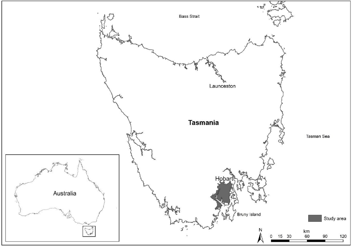
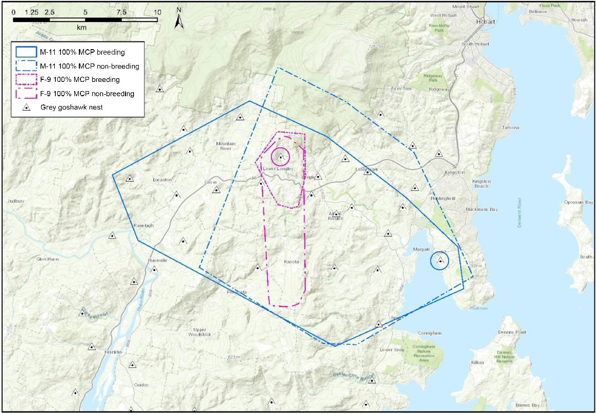
The study area was located in the Huon Valley and D’Entrecasteaux Channel areas, approximately 35 km south-west of the capital city of Hobart (coordinates: 42.98°S, 147.08°E), south-east Tasmania, Australia (Fig. 1). The area comprises a complex mosaic of agricultural, urban and rural areas, interspersed with river valleys and large tracts of native forest. Low lying coastal areas, fertile river mouths and river valleys were cleared of forest and now support a high proportion of human dwellings (Department of Natural Resources and Environment Tasmania 2024). Most of the land is freehold property with complex land use types, zoning and land title structure (Huon Valley Council 2024). Fruit growing, grazing, stock rearing and various other agricultural activities take place. Commercial logging occurs in the surrounding forests. Hardwood and softwood plantations have been established on public and private land to support the logging industry, particularly in lower parts of the Huon Valley and Southern Forests. The human population of the two municipalities (Kingborough and Huon Valley) that encompass the study area was approximately 60,254 in 2023/2024, with most in major towns such as Kingston, Huonville, Margate, Cygnet (Australian Bureau of Statistics 2023; Kingborough Council 2024).
The area experiences a temperate maritime climate with cold winters and warm to hot summers, with high cloud cover throughout the year. Mean minimum daily temperature in June was 2.2°C and mean maximum daily temperature in January was 23.6°C for the 19-year period between 2004 and 2024 in Grove (Bureau of Meteorology 2024). Average annual rainfall in Grove for the 30-year period between 1991 and 2020 was 502–1051 mm (Bureau of Meteorology 2024). Elevation in the study area ranges from sea level to 831 m above sea level (ASL) with Snug Tiers being the major topographic feature. Vegetation is predominantly wet and dry sclerophyll forests (eucalypt forest), non-eucalypt forests, coastal heathland and sedgeland; however, small amounts of temperate rainforest occur in areas that receive relatively high rainfall. (Kitchener and Harris 2013). Rainforest is dominated by myrtle (Nothofagus cunninghamii), sassafras (Atherosperma moschatum) and celery top pine (Phyllocladus aspleniifolius). Eucalypt forests are dominated by stringybark (Eucalyptus obliqua). swamp gum (E. regnans), blue gum (E. globulus), manna gum (E. viminalis), white peppermint (E. pulchella), black peppermint (E. amygdalina) and silver peppermint (E. tenuramis). Non-eucalypt forests are predominantly silver wattle (Acacia dealbata) and blackwood (Acacia melanoxylon) and common midstory forest species are silver wattle (A. dealbata), blackwood (A. melanoxylon), native cherry (Exocarpus cuppressiformis), musk (Olearia argophylla) and dogwood (Pomaderris apetala).
Telemetry
We trapped 13 (11 females, two males) adult grey goshawks during the breeding season in 2022, and two adult females in 2023. They were captured approximately 100–500 m away from known active nest sites during the nestling stage to ensure breeding adults were fitted with transmitters. We used a remote activated bow-net to trap individuals that were enticed/lured to the trap site by (1) roadkill carcases or (2) a combination of call playback (i.e. broadcasting pre-recorded grey goshawk vocalisations through a speaker) and a taxidermy grey goshawk as a visual lure. We fitted 10 g, solar rechargeable GPS transmitters (Model ES 420, Cellular Tracking Technologies, Rio Grande, NJ, USA) to goshawks with backpack style harnesses made of 6 mm Teflon ribbon (total weight < 3% of body mass). Transmitters were programmed on an adaptive duty cycle and recorded location fixes every 60–720 min, depending on battery charge levels, from 1 h before sunrise to 1 h after sunset every day. In general, fixes were obtained every 120 min during the breeding season (i.e. summer months) and between 180 and 720 min in the non-breeding season (i.e. winter months, due to short daylength and low solar intensity). The transmitters ‘checked-in’ once per day and uploaded location fixes (GPS coordinates) automatically to a graphical user interface via the 3G/4G GSM network.
Processing
Trapped goshawks were assessed for body condition based on a pre-defined scoring system developed in consultation with a qualified veterinarian. The scoring system ranged from 0 to 5, with 0 being very poor condition (i.e. emaciated with an exposed keel and minimal breast muscle) and 5 being excellent (keel not exposed, prominent breast muscle and significant fat deposits present). Individuals with a body condition score of 3 or higher were deemed to be in good condition and suitable to be fitted with a transmitter. Birds in poor condition (those with a score of 3 or less) were weighed, leg banded and released without a transmitter attached. We weighed, leg banded, collected morphometric measurements (to the nearest mm) and extracted blood samples from birds in good condition. GPS transmitters were then fitted, and the birds were released at the capture site. Processing time was 40–60 min. All goshawks trapped were banded with Australian Bird and Bat Banding Scheme (ABBBS) stainless steel leg bands around the tarsus. Females were fitted with size 14 bands and males were fitted with size 12 bands, as per ABBBS guidelines (ABBBS 2020).
Blood samples for molecular sex determination were taken from the brachial vein with a 25-gauge butterfly canula. 0.5 mL of blood was collected from field sexed females (n = 13) and 0.3 mL from field sexed males (n = 2). To extract blood, the area around the brachial vein was sterilised with an alcohol swab (100% isopropyl alcohol) and pressure was applied to the area post-extraction with a sterile swab. Blood samples were stored in vials containing 0.25 mL of lysis buffer solution prior to DNA extraction. DNA extraction, PCR and molecular sexing was conducted at the genetics laboratory of the University of Tasmania.
Home range
We used 100% MCP to estimate overall home range size (i.e. the habitat extent) (Burt 1943), of grey goshawks during the breeding and non-breeding season. We used this method as it is commonly used and allows generalised comparisons with other raptor home range studies (Mohr 1947). We used 50%, 75% and 95% fixed-kernel density (KD) to estimate core areas, as this method is well suited for such tasks with GPS telemetry data (Kie et al. 2010; Tétreault and Franke 2017). Fixed-kernel density estimation is particularly sensitive to bandwidth selection, whereas kernel choice (i.e. normal, bi-weight, quadratic etc.) has little influence on density estimates (Hall et al. 1991; Turlach 1993; Altman and Léger 1995). We were more interested in density probabilities (utilisation distributions – UD) (Worton 1989) than overall home size, so we used the default bandwidth (href) based on Silverman’s Rule of Thumb bandwidth estimation formula, as it minimises smoothing (Silverman 1986; Bowman and Azzalini 1997; ESRI Inc. 2020). This is important if the distribution of the data is unknown, as over-smoothed unimodal data will provide relatively large, inaccurate estimates (ESRI Inc. 2020). Moreover, over-smoothing can change multi- or bimodal density distributions to unimodal and remove important information (Wand and Jones 1994; Sheather and Jones 1999). Silverman’s algorithm (href) calculates the search radius for each data set independently based on the number and spatial distribution of input points, and corrects for outliers to minimise the search radius (Silverman 1986). It uses a quartic (biweight) kernel, whereby calculations are applied to the centre of every cell in the output raster layer to estimate the density of points (Silverman 1986). We used the default population field, output cell size of 5, square kilometres as the area unit factor, and planar as the method parameter. All home range analyses were conducted using the Kernel Density tool in ArcMap 10.8.1. (ESRI Inc. 2020).
Prior to conducting home range analyses, we downloaded full data sets for each goshawk from the graphic user interface (GUI) platform and removed erroneous or inaccurate data points (points with horizontal displacement of position (HDOP) values > 3). Location fixes recorded during the first 48 h post-capture/transmitter attachment were also removed to allow the birds to acclimate. Fix locations used in home range analyses were 60–720 min apart, which ensures independence and avoids errors associated with autocorrelation (Dale and Fortin 2002; Silva et al. 2022). To estimate goshawk home range sizes for breeding and non-breeding seasons independently, we defined the breeding season as 1 October−14 February and non-breeding as 1 April−1 September, based on observations of breeding phenology in our study area. For example, most eggs are laid around mid-October and juvenile goshawks have generally dispersed from natal nests by the end of February (Young unpubl. data). Telemetry locations recorded outside of these defined periods were excluded from home range analyses as they were transitional periods, and thus space use and movements could not be assigned reliably to breeding or non-breeding behaviour. We assumed all locations within a 200 m radius of active nest trees during the breeding season to be breeding related activities. All other locations are assumed to be ‘foraging’ although we are aware and acknowledge that some may be associated with other behaviours such as breeding activities, preening, displaying and territory defence.
Number of nests per breeding area and inter-nest distances
To determine the number of nests per goshawk breeding territory and calculate inter-nest distances, we used nest site locations in the study area that were identified previously, as part of a larger study (see Young and Kirkpatrick 2024). All nest locations were mapped, and we then generated 590 m radius buffer zones around each active nest tree using the Buffer Tool in ArcMap 10.8.1 (ESRI Inc. 2020) (see Young and Kirkpatrick 2024 for descriptions of how buffer zone size was determined). We then counted the number of nests recorded within each buffer zone and allocated each with a unique identifier number (UI). Distances between nests within each buffer zone were then measured in metres using the Measure Tool in ArcMap (ESRI Inc. 2020). Several nests outside of the defined buffer zones were also included because they were used for breeding during the study period by resident females (from known territories) whilst they were equipped with GPS transmitters.
Results
Nests
In total, 153 grey goshawk nests were identified in 73 breeding territories. Mean number of nests per breeding territory was 2.0 (s.d. = 1.0, median = 1.0, range = 1.0–6.0). Median distance between nests within breeding territories was 78.0 m (s.d. = 256.4, mean = 186.8, range = 1.8–915.0). Maximum number of nests in a nest stand (defined as a patch of forest within a breeding territory that contains one or more nest trees) was six and the maximum number of nest stands identified in a breeding territory was three. Area (100% MCP) of the largest individual nest stand identified was 0.54 ha (0.005 km2) and contained six nests. The largest area (100% MCP) containing active and alternate nests (n = 6 nests in three forest stands) was 21.18 ha (0.21 km2).
Home range
We calculated home ranges for 15 (13 females, two males) breeding grey goshawks equipped with GPS trackers between December 2021 and October 2023 (Table 1). Home range estimates are based on a mean number of 1080 ± s.d. 472.5 fixes in the breeding season and 667 ± s.d. 381 fixes in the non-breeding season (Table 2). GPS data was collected throughout a full breeding cycle for six females and one male (Table 1).
| Year | 2021 | 2022 | 2023 | |||||||||||||||||||||
|---|---|---|---|---|---|---|---|---|---|---|---|---|---|---|---|---|---|---|---|---|---|---|---|---|
| Dec | Jan | Feb | Mar | Apr | May | Jun | Jul | Aug | Sep | Oct | Nov | Dec | Jan | Feb | Mar | Apr | May | Jun | July | Aug | Sep | Oct | ||
| Sex/ID | ||||||||||||||||||||||||
| F-2 | B | B | B | B | B | B | B | |||||||||||||||||
| F-3 A | B | B | B | B | B | B | ||||||||||||||||||
| F-4 B | B | B | B | B | B | |||||||||||||||||||
| F-5 | B | B | B | B | B | B | B | |||||||||||||||||
| F-6 B | B | B | B | B | B | B | ||||||||||||||||||
| F-7 | B | B | B | B | B | B | ||||||||||||||||||
| F-8 C | B | B | B | B | B | B | ||||||||||||||||||
| F-9 | B | B | B | B | B | B | B | |||||||||||||||||
| F-10 | B | B | B | B | B | B | ||||||||||||||||||
| F-12 B | B | B | B | B | B | B | ||||||||||||||||||
| F-13 | B | B | B | B | B | B | B | |||||||||||||||||
| F-14 | B | B | B | B | B | B | B | |||||||||||||||||
| F-15 B | B | B | B | B | B | B | B | |||||||||||||||||
| M-1 B | B | B | B | B | B | B | B | |||||||||||||||||
| M-11 | B | B | B | B | B | B | B | |||||||||||||||||
Months highlighted in bold italic text indicate the defined breeding periods for this study.
Sex: F, female; M, male; ID, trapping order; B, breeding (incubating or with dependent chick/s or young).
| Study area | Sex/ID | Home-range (km2) | Home-range (km2) | |||||||||
|---|---|---|---|---|---|---|---|---|---|---|---|---|
| Breeding | Non-breeding | |||||||||||
| No. fixes | 50% KD | 75% KD | 95% KD | MCP 100% | No. fixes | 50% KD | 75% KD | 95% KD | MCP 100% | |||
| Dover | F-2 | 1012 | 0.19 | 2.19 | 2.98 | 15.10 | 569 | 0.67 | 2.22 | 13.65 | 58.80 | |
| Port Huon | F-3 | 718 | 0.17 | 1.11 | 3.72 | 5.00 | – | – | – | – | – | |
| Kermandie | F-4 | 897 | 0.18 | 0.43 | 2.01 | 3.96 | 207 | 0.34 | 1.09 | 2.08 | 181.90 | |
| Cairns Bay | F-5 | 2165 | 0.20 | 2.60 | 6.00 | 15.10 | 497 | 1.40 | 2.60 | 7.40 | 27.00 | |
| Geeveston | F-6 | 1201 | 0.38 | 0.44 | 3.89 | 48.20 | 514 | 0.90 | 2.51 | 6.68 | 16.30 | |
| Franklin | F-7 | 594 | 0.20 | 0.57 | 3.10 | 46.90 | 391 | 0.63 | 1.52 | 5.51 | 28.60 | |
| Ranelagh | F-8 | 1460 | 0.20 | 0.50 | 6.90 | 14.90 | 627 | 0.40 | 1.70 | 5.96 | 45.82 | |
| Lower Longley | F-9 | 2384 | 0.20 | 1.61 | 4.16 | 15.10 | 1245 | 0.32 | 0.89 | 6.10 | 30.60 | |
| Cygnet | F-10 | 2507 | 0.32 | 1.67 | 4.04 | 16.00 | 1238 | 0.41 | 1.60 | 5.23 | 10.20 | |
| Lower Longley | F-12 | 486 | 0.21 | 1.33 | 4.32 | 12.70 | – | – | – | – | – | |
| Margate | F-13 | 400 | 0.26 | 3.70 | 4.12 | 14.41 | 382 | 2.30 | 8.30 | 9.70 | 14.40 | |
| Gardners Bay | F-14 | 352 | 0.32 | 0.94 | 2.15 | 29.60 | 127 | 0.82 | 2.71 | 4.10 | 61.10 | |
| Cygnet | F-15 | 507 | 0.42 | 0.97 | 2.77 | 10.40 | – | – | – | – | – | |
| Mean | F | 1129 | 0.25 | 1.39 | 3.86 | 19.03 | 580 | 0.82 | 2.51 | 6.64 | 47.47 | |
| s.d. | F | 770 | 0.08 | 0.97 | 1.39 | 14.06 | 381 | 0.62 | 2.13 | 3.17 | 50.44 | |
| Range min- | F | 352 | 0.17 | 0.43 | 2.01 | 3.96 | 127 | 0.32 | 0.89 | 2.08 | 10.20 | |
| max | 2507 | 0.42 | 3.70 | 6.90 | 48.20 | 1245 | 2.30 | 8.30 | 13.65 | 181.90 | ||
| Surges Bay | M-1 | 1155 | 0.36 | 4.08 | 12.95 | 89.2 | – | – | – | – | – | |
| Howden | M-11 | 908 | 0.21 | 3.15 | 10.44 | 231.8 | 754 | 2.70 | 5.07 | 35.90 | 219.00 | |
| Mean | M | 1032 | 0.29 | 3.62 | 11.70 | 160.50 | 754 | 2.70 | 5.07 | 35.90 | 219.00 | |
| s.d. | M | 175 | 0.11 | 0.66 | 1.77 | 100.83 | 0 | 0.00 | 0.00 | 0.00 | 0.00 | |
| Range min- | M | 908 | 0.21 | 3.15 | 10.44 | 89.20 | 754 | 2.70 | 5.07 | 35.90 | 219.00 | |
| max | 1155 | 0.36 | 4.08 | 12.95 | 231.80 | 754 | 2.70 | 5.07 | 35.90 | 219.00 | ||
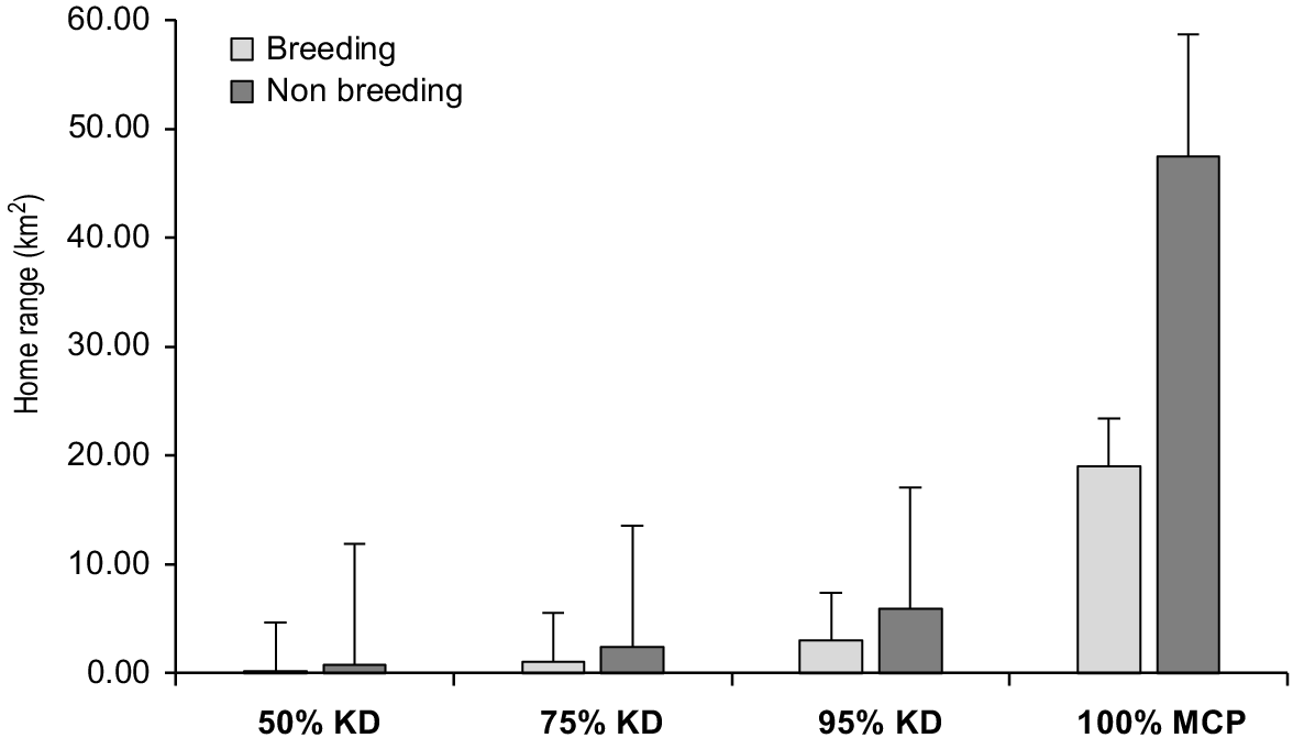
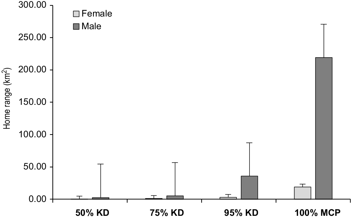
Home range sizes differed between individuals, sex and season (Table 2; Figs 2 and 3). Mean 100% MCP home range size of females during the breeding season was 19.03 ± s.d. 14.06 km2 and 47.47 ± s.d. 50.44 km2 in the non-breeding period. Mean 100% MCP home range size of males was 160.50 ± s.d. 100.83 km2 in the breeding period and 219.00 ± s.d. 0.00 km2 in the non-breeding period (Table 2). KD home range estimates were smaller than MCP estimates. Mean KD core area size of females during the breeding period were (50%, 0.25 ± s.d. 0.08 km2; 75%, 1.39 ± s.d. 0.97 km2; 95%, 3.86 ± s.d. 1.39 km2) and (50%, 0.82 ± s.d. 0.62 km2; 75%, 2.51 ± s.d. 2.13 km2; 95%, 6.64 ± s.d. 3.17 km2) in the non-breeding period (Table 2). Mean KD core area size of males in the breeding period were (50%, 0.29 ± s.d. 0.11 km2; 75%, 3.62 ± s.d. 0.66 km2; 95%, 11.70 ± s.d. 1.77 km2) and (50%, 2.70 ± s.d. 0.00 km2; 75%, 5.07 ± s.d. 0.0 km2; 95%, 35.90 ± s.d. 0.0 km2) in the non-breeding period (Table 2).
Utilisation distributions
KD utilisation distributions (i.e. core areas) of females were unimodal and were centred on the nest tree during the early breeding season (i.e. nestling stages) and transitioned to bimodal in general later in the season in response to shifts in activity centres (Fig. 4). The shifts reflected decreased fidelity to the nest site and young, and increasing distances travelled from the nest to preferred foraging locations. Utilisation distributions of females in the non-breeding period were bimodal initially but progressed to unimodal in the middle of winter and into the pre-breeding season. Male utilisation distributions followed a similar pattern.
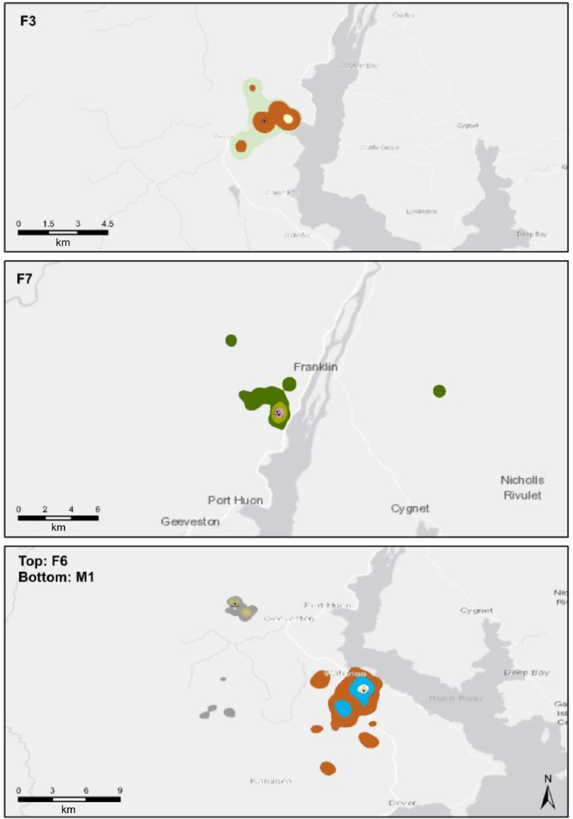
Kernel Density (KD) home-range estimates of four (three female/one male) grey goshawks during the breeding season in south-east Tasmania, Australia. Inner coloured areas represent 50% KD isopleths, central areas 75% and outer areas 95%. Note the larger core areas of the male goshawk (M-1) compared to the females (F-3, F-6, F-7). Also note the bimodal utilisation distribution (i.e. two core 50% KD areas) for F-6, bimodal 75% KD distribution for M-1 and F3. 50% KD core areas were centred on nest sites generally but also on alternate nest sites and preferred foraging areas. For example, the 50% KD core area of F-3 is not centred on the nest, but on a location east of the nest that contained abundant European rabbits (Oryctolagus cuniculus). This location also contained an alternate nest and was a post-fledging area used by juvenile grey goshawks after they left the natal nest area.
Movement patterns and transit distances
Tracked grey goshawks were range residents (i.e. did not migrate) throughout the year and space use (i.e. 50% and 75% KD core areas) was concentrated on important resources such as nest trees, alternate nest trees and preferred foraging locations within a few kilometres of the nest tree. Movement patterns associated with these features were highly recursive. Female goshawks occasionally undertook long range excursions (~5–13 km) away from their nests and nestlings for 1–4 days in the breeding season and others abandoned their nest sites temporarily post-breeding season and undertook long range excursions (~5–54 km from the nest) for a week to several weeks at a time before returning. In contrast, males undertook long range excursions more frequently but for shorter periods of 1–4 days at a time. In the breeding season, the farthest distance travelled from the nest by a female goshawk was 12.9 km (F-6) and the farthest for a male was 11.6 km (M-11). In the non-breeding season, the farthest distance travelled from the nest by a female was 54.0 km (F-4) and the farthest for a male was 17.6 km (M-11). Maximum daily distance travelled by a male was 22.3 km and 57.4 km by a female. Highest elevation recorded for a male was 800 m ASL (mean 797 ± 4.2 m ASL) and the highest for a female was 1138 m ASL (mean 851.6 ± 221.6 m ASL). Ranging behaviour of male goshawks was extensive and generally circular, whereas female movements were highly directional and linear (Fig. 5). Males ranged over small areas near the nest and large areas around the outer edges of their home ranges, whereas female movements were more specific and tended to focus on certain locations within 1 km of the nest tree and remote areas many kilometres away. The tracking data also showed that males often visited nest sites of other grey goshawks in our study area, whereas females strictly avoided them.
Discussion
This study provides the first home range estimates for grey goshawks throughout the species’ range using GPS telemetry. The use of high-resolution GPS technology provides more reliable and accurate estimates of home range sizes for the species than previously reported estimates based on radiotelemetry (Burton and Olsen 2000). Moreover, our results are based on a mean number of 873 locations per bird, our data was collected independently of environmental variables, and a higher number (n = 15) of individuals were tracked (Burton and Olsen 2000). We also tracked goshawks for a longer duration than previous studies (Burton and Olsen 2000). For example, we tracked seven goshawks throughout a full breeding cycle, all of which bred and raised young successfully whilst equipped with transmitters.
Using GPS technology, we documented grey goshawks using large home ranges with movement patterns varying at different times of the year. The results showed that female breeding season home range size (MCP) was 60% smaller than non-breeding season home ranges. Female home range size was 88% smaller than home ranges of males in the breeding season and 78% smaller in the non-breeding season. Although our results for male goshawks over a full breeding cycle (i.e. breeding and non-breeding seasons) are limited to one individual, home range size of both males that we tracked were very large, such that our results are probably representative of male home range size and therefore the differences in home range sizes between the sexes generally. Indeed, the differences in home range sizes we recorded between male and females and between breeding and nonbreeding seasons are consistent with other home range studies on goshawks elsewhere (Boal et al. 2003; Roberson et al. 2004; Kenward 2006; Moser and Garton 2019; Blakey et al. 2020).
Home range estimates we obtained are much larger than those reported for grey goshawks in sub-tropical areas of Australia, where Burton and Olsen (2000) reported mean MCP home range sizes of 80 ha for males and 11 ha for females in the breeding season and 105 ha for males and 587 ha for females in the non-breeding season. Core home range estimates in their study are also much smaller than our estimates. Burton and Olsen (2000) attributed the small home range sizes in their study to the richness of their study area. If this is the case, the large home ranges we obtained implies that our study area (i.e. temperate and maritime) is relatively low quality (i.e. low productivity) habitat for goshawks in comparison to sub-tropical areas. Areas at lower latitudes are known to support relatively high primary productivity so this may be a reason for the observed differences, but it is unlikely. We propose that the differences in home sizes probably reflect the tracking method used (GPS/VHF) and the fact we tracked goshawks for a much longer period and our sample size was larger. It could also reflect the larger size of grey goshawks in Tasmania compared to individuals on the mainland (Baker-Gabb 1984; Burton and Alford 1994) as home range size of raptors is known to increase linearly with body size (Newton 1979; Newton 1986; Peery 2000). Home range estimates we obtained for grey goshawks are larger than estimates for brown goshawks (Accipiter fasciatus) (Burton and Olsen 2000) and smaller than estimates for red goshawks (Erythrotriorchis radiatus) (Aumann and Baker-Gabb 1991) in Australia. Tracking of two adult red goshawks fitted with radiotelemetry established that the breeding home range was approximately 120 km2 and 200 km2 for the female and the male, respectively (Aumann and Baker-Gabb 1991; DCCEEW 2023). Czechura (1996) recorded red goshawks flying 6–10 km to hunting areas, which is similar to what we recorded for grey goshawks. More recent GPS tracking work showed red goshawks travelled more than 1500 km from the nest and flew to heights of > 1000 m ASL (MacColl et al. 2021). The maximum distance grey goshawks travelled from the nest was 54 km and the maximum elevation recorded for a male was 800 m ASL and the highest for a female was 1138 m ASL.
Grey goshawk home ranges that we recorded are smaller than estimates reported for the larger northern goshawk (Accipiter gentilis) in forested areas of the Unites States based on GPS data (Moser and Garton 2019; Blakey et al. 2020). However, northern goshawk home ranges in urban areas were smaller (Rutz 2006) than our estimates for grey goshawks, and smaller than estimates for northern goshawks in more natural areas in the United States (Boal et al. 2003). The relatively small home range size of northern goshawks in urban areas implies food abundance and availability is a major factor affecting home range size (Rutz 2006; Rutz 2008). Indeed, urban areas are recognised as highly productive foraging locations for certain raptors, especially small bird and mammal specialists like goshawks (Boal and Dykstra 2018).
In this study, grey goshawk home range size varied between individuals, between males and females and between breeding and non-breeding periods, as other studies have found (Kenward 2006). Home range sizes also differed significantly between the two estimators, as expected, with KD estimates being much smaller than MCP estimates. We propose that the high level of variance in home range sizes (excluding differences between MCP and KD) can be attributed to several factors, such as the density of GPS fixes (i.e. higher and lower utilisation rates of certain areas), the duration of tracking, breeding phenology and the month that transmitters were attached (see Table 1). Differences in the quality of home range (i.e. primary productivity, proportions of habitat types, prey abundance) and breeding success are also likely to have affected home range size, as other studies on goshawks and raptors in general suggest (Newton 1979; Newton 1986; Kenward 2006). For example, Moser and Garton (2019) showed that northern goshawk home ranges were a function of breeding success and proportion of cover types within the home range. They found that home range sizes of both sexes were larger when breeding was unsuccessful, male home ranges were larger than females, and the sexes selected home ranges with differing proportions of forest types and edge ratios. Interestingly, the larger home range size reported by Moser and Garton (2019) in response to unsuccessful breeding is similar to the rapid increases in home range size we recorded for female grey goshawks at the end of the breeding season.
Our results compare surprisingly well with estimates of inter-nest distances for the species in Tasmania reported in a previous study by Young and Kirkpatrick (2024). For example, they reported a minimum inter-nest distance between active nests of 1079 m (i.e. a radius of 539.5 m around each nest tree), which closely matches the approximate mean radius of the 75% KD estimates (~577 m) around nest trees we obtained. This provides indirect evidence that grey goshawks are indeed territorial, and our mean 75% core area estimate closely represents the area that is defended from conspecifics. Importantly, the 75% core area can therefore be defined as the ‘Breeding Territory’ with confidence in a prescriptive nest reserve system like the ‘Goshawk Management Area’ system that is used in the United States for management and conservation of northern goshawks (Reynolds et al. 1992; Coast Forest Conservation Initiative (CFCI) 2012).
Ranging behaviour
We found that grey goshawk core areas (50% and 75% KD) are centred on active nest trees, alternate nest trees, and preferred foraging locations. Movement patterns of both sexes were highly recursive, indicating these areas are extremely important to breeding adult goshawks, and they have detailed knowledge of their home ranges and prime foraging locations. It also demonstrates that certain locations within their home ranges are superior for foraging compared to other areas, given the specificity and intensity of utilisation. Future studies should focus on characterising these areas. We also recorded goshawks undertaking long range excursions away from their nest sites for days to several weeks. Other studies have reported similar movement patterns and behaviours (Moser and Garton 2019; Blakey et al. 2020). Surprisingly, the temporary abandonment of nest sites by female goshawks and the subsequent long-range excursions for extended periods at the end of the breeding season coincided with the onset of the dispersal stage of juveniles (i.e. 3–4 weeks post-fledging). Indeed, by the time the females returned to their nest sites, juvenile goshawks had dispersed from the natal nest areas and could not be located (confirmed by site visits). This strongly suggests parents initiate and facilitate dispersal of juveniles by abandoning the natal nest area and ceasing food provisions. Moreover, our KD analyses identified some of the areas the goshawks visited frequently during these long-range excursions as 75% core areas. This highlights that they are prime foraging sites and implies long-range excursions are extended foraging trips to exploit rich foraging grounds. Regaining condition after months of provisioning food to their young is probably a major driver of these post-breeding, long range excursions. Moreover, these long-range movements highlight the importance of temporal resolution in home range studies. For example, if these movements weren’t captured within the period we defined as ‘breeding’, home range estimates of females in the breeding season would have been significantly smaller. Future studies should estimate home range size at finer temporal scales in the future.
We observed notable differences in ranging behaviour between male and female goshawks. Males appeared to roam throughout their expansive home ranges and around the outer edges or boundaries, whereas female movements were more directional and focussed on specific locations within a few kilometres of the nest and in very remote areas, as if they were familiar or known to them prior to departing (i.e. they possess a detailed cognitive map of their home range and a much larger area). The tracking data also indicated that males frequently visited nest sites (active and alternate) of other grey goshawk pairs (known to us and mapped) in our study area, some of which were up to 8 km away. Females, on the other hand, strictly avoided nest sites of neighbouring pairs and other nest sites in the study area, including those of brown goshawks (Tachyspiza fasciatus), presumably in response to the aggressiveness of females towards each other. Blakey et al. (2020) reported similar behaviours by GPS tracked northern goshawks and proposed that males may be seeking extra-pair copulations, exploiting resources at nest sites or undertaking reconnaissance.
Nests
This study confirmed that grey goshawks use and maintain multiple nests in multiple nest stands within their territories, which concurs with other studies on goshawks elsewhere (Burton et al. 1994; Penteriani 2002; Andersen et al. 2005; Kenward 2006). Nest stands are easily distinguished from surrounding forest with a trained eye by obvious differences and/or changes in forest structure, especially, proportionately more large trees (i.e. diameter at breast height (dbh) > 70 cm), lower basal area, most trees have high branchless trunk height and high canopy cover (Young and Kirkpatrick 2024). Other features, such as watercourse junctions and concave landforms, are also characteristic of grey goshawk nest stands (Young and Kirkpatrick 2024; D. Young, S. Harwin, J. B. Kirkpatrick, unpubl. data). The maximum distance we recorded between nests in a breeding territory was 915 m and mean distance was 186 m. Consequently, nest searches to identify alternate nests in goshawk breeding territories should be undertaken within a 915 m radius from known nest tree locations. If searches are not feasible within this radius, at a minimum, they should be conducted within a 300 m radius of a known nest tree as the vast majority of nests are within this distance of active nest trees.
Importantly, the largest area (100% MCP) containing active and alternate nests (n = 6 nests in three forest stands) was 21.18 ha (0.21 km2) which is similar to the mean core area size (0.25 km2) estimated from the GPS telemetry data. This indicates that core areas of use correspond to the size or area encompassing all nest trees within a breeding territory. Therefore, the MCP area encompassing all nest trees can be used as an approximation to implement core nest reserves in areas where telemetry data is not available.
This study identified and quantified core areas of adult grey goshawks during the breeding season whilst they were provisioning young. The core area estimates (50%, 75%, 95% isopleths) are based on utilisation distributions of these goshawks and therefore encapsulate essential resources and cater for their spatial requirements. They can therefore be used with confidence as the basis for the design of prescriptive nest reserves for the species.
We propose and recommend a ‘Grey Goshawk Management Area’ system be implemented to assist with conservation and management of the species in the future (see Figs 6 and 7 below). It is a concentric area-based system similar to what has been used for management of northern goshawks in the United States for decades (Coast Forest Conservation Initiative (CFCI) 2012).
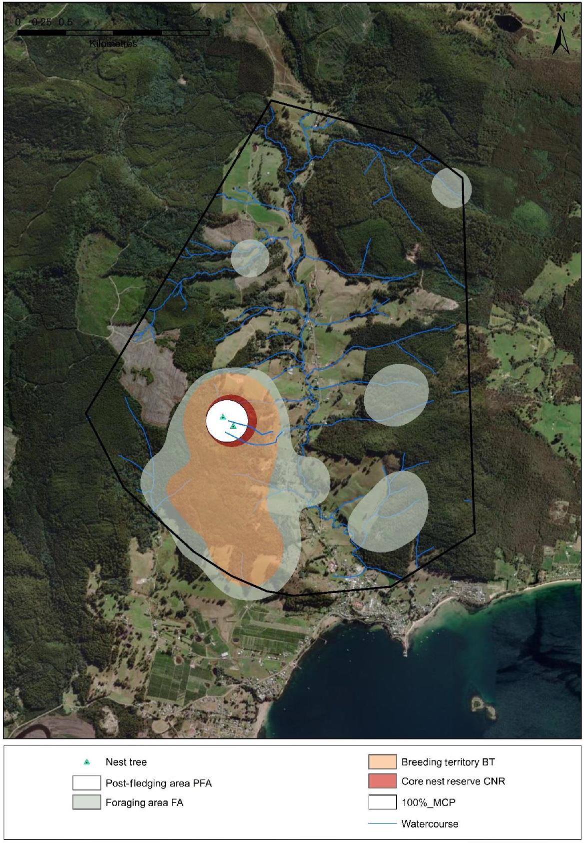
Conceptualised design (not drawn to scale) of a ‘Grey Goshawk Management Area’ (GGMA) system in Tasmania. The size of the post-fledging area was estimated based on direct observations of juvenile grey goshawks at active nest sites (Young unpubl. data) and is supported by McClaren et al. (2005). The design concept was adapted from Coast Forest Conservation Initiative (CFCI) (2012).
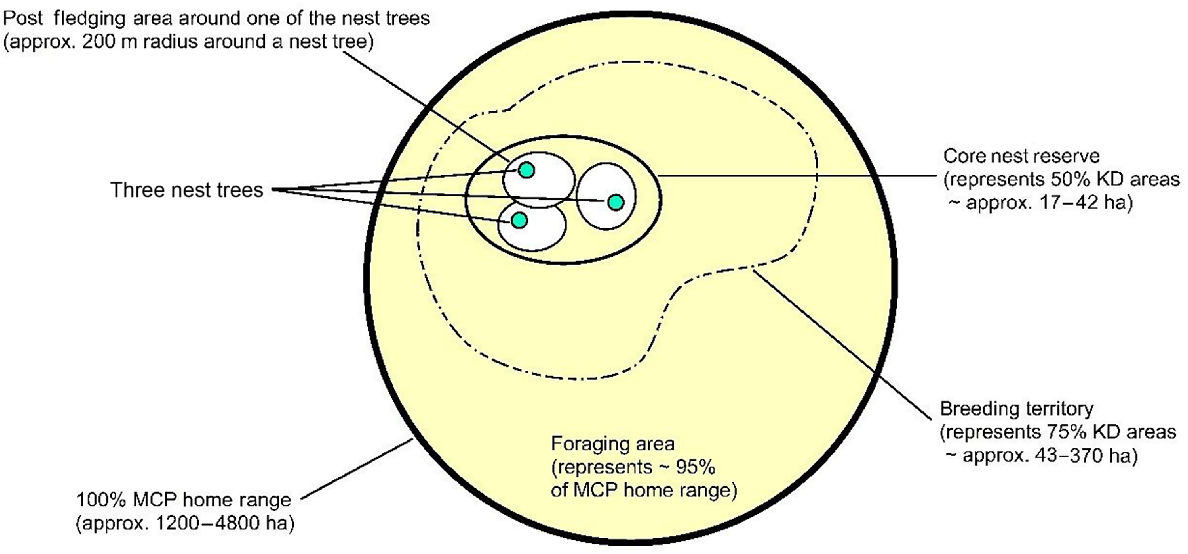
Conceptualised design for a ‘Grey Goshawk Management Area’ (GGMA) in Tasmania based on core area estimates of GPS tracked individuals and known nest trees.
To facilitate a species-specific design for grey goshawks, we recommend the following:
implement ‘Core Nest Reserves’ (CNR) based on 50% KD core area estimates
implement ‘Breeding Territory’ (BT) management zones based on 75% KD core area estimates
implement ‘Foraging Area’ (FA) management zones based on 95% core area estimates.
Recommendations provided above are based on mean KD core area estimates of female grey goshawks during the breeding season (Table 2). Conceptualised examples of a design are provided in Figs 6 and 7 to assist with site specific design and implementation of the proposed management system.
A ‘Grey Goshawk Management Area’ system is likely to be an appropriate conservation management strategy for the species as it is evidence-based and caters for the spatial requirements and essential resources of breeding pairs and juvenile goshawks prior to dispersal from natal nests. It also provides a framework to integrate existing management strategies and implement new ones as new data or information on the species becomes available.
CNR – Core Nest Reserve 50% KD – Core nest reserves encompass the active nest tree, alternate nest trees and post-fledging areas.
BT – Breeding Territory 75% KD – These management zones encompass entire breeding territories (i.e. the area defended from conspecifics), which includes multiple forest stands that each contain several nest trees.
FA – Foraging Area 95% KD – These management zones are areas outside of core nest reserves (CNRs) and breeding territory (BTs) zones.
100% MCP – All of the above areas fall within the 100% MCP home range and thus should be managed as a functioning integrated unit, with a strong focus on protecting goshawk nest sites and nesting habitat, facilitating desired forest conditions and maintaining goshawk food webs (Coast Forest Conservation Initiative (CFCI) 2012).
Two nest trees depicted (mean inter-nest tree spacing = 198 m).
Post fledging Area (PFA) size (200 m radius around each nest tree) = 12.56 ha
Core Nest Reserve (CNR) Area size = 23.0 ha (50% KD)
Breeding Territory (BT) Management Zone size = 191.6 ha (75% KD)
Foraging Area (FA) Management Zone size = 328.4 ha (95% KD)
Goshawk Management Area size = 1510.2 ha (100% MCP)
The GGMA design incorporates logical features such as streams, riparian habitats, mature forest and forested slopes with south-east aspects, which are important to the species.
Note contiguity of forested habitat in the Breeding Territory Management Zone to the south of the core nest reserve.
This GGMA design represents a ‘low to medium risk of abandonment’ scenario as forest harvesting is occurring outside of the Foraging Area Management Zone but anthropogenic disturbance is occurring within Foraging Area Management Zone and the Breeding Territory (BT) Management Zone. Note: a nest 900 m to the north of the current two nest sites was abandoned in 2022, possibly due to disturbance.
Detrimental activities such as removal and alteration of vegetation within core nest reserves should be strictly avoided. Direct disturbance should be strictly avoided within post-fledging areas (i.e. within a 200 m radius of nest trees).
Data availability
Data sharing is not applicable. Raw data is not available due to sensitivities in relation to locations of an endangered species.
Conflicts of interest
The primary author declares that there are no known conflicts of interest, financial or personal, that influenced the work presented in this manuscript. Co-author deceased; no conflicts of interest available.
Declaration of funding
Funding was generously provided by Timberlands Pacific, Sustainable Timber Tasmania, Birdlife Australia Stuart Leslie Award, SFM Environmental Solutions, Tasmanian Forest Practices Authority, Tassal Limited, Birds Australia Raptor Research Group (BARG) and the Robinson Holdsworth Foundation.
Acknowledgements
This study was conducted under University of Tasmania animal ethics permit No. 23886 and Department of Natural Resources and Environment Scientific Permits TFA 21202 and TFA 22490. Dr James Pay, Dr Amelia Koch and Nick Mooney provided assistance and advice on study design, model development and creation of GIS layers. We thank Adam Smolenski from the University of Tasmania Molecular Genetics Central Science Laboratory for conducting DNA extraction and molecular sexing of goshawk blood samples. We also thank Nick Mooney and Dr Phil Bell for reviewing drafts of the manuscript. And landowners who kindly allowed access to grey goshawk nests on their property and landowners, colleagues and members of the public that provided nest locations or information that led to a nest being located.
References
Altman N, Léger C (1995) Bandwidth selection for kernel distribution function estimation. Journal of Statistical Planning and Inference 46(2), 195-214.
| Crossref | Google Scholar |
Andersen DE, DeStefano S, Goldstein MI, Titus K, Crocker-Bedford C, Keane JJ, Anthony RG, Rosenfield RN (2005) Technical review of the status of northern goshawks in the western United States. Journal of Raptor Research 39, 192-209.
| Google Scholar |
Baker-Gabb DJ (1984) Morphometric data and dimorphism indices of some Australian raptors. Corella 8(3), 61-63.
| Google Scholar |
Bilney RJ, White JG, L’Hotellier FA, Cooke R (2011) Spatial ecology of Sooty Owls in south-eastern Australian coastal forests: implications for forest management and reserve design. Emu - Austral Ornithology 111, 92-99.
| Crossref | Google Scholar |
BirdLife International (2016) ‘Accipiter novaehollandiae’. IUCN red list of threatened species. Available at https://dx.doi.org/10.2305/IUCN.UK.20163.RLTS.T22727714A94958201.en [accessed 20 May 2022]
Blakey RV, Siegel RB, Webb EB, Dillingham CP, Johnson M, Kesler DC (2020) Northern Goshawk (Accipiter gentilis) home ranges, movements, and forays revealed by GPS-tracking. Journal of Raptor Research 54(4), 388-401.
| Crossref | Google Scholar |
Boal CW, Andersen DE, Kennedy PL (2003) Home range and residency status of northern goshawks breeding in Minnesota. The Condor 105, 811-816.
| Crossref | Google Scholar |
Boggie MA, Butler MJ, Sesnie SE, Millsap BA, Stewart DR, Harris GM, Broska JC (2023) Forecasting suitable areas for wind turbine occurrence to proactively improve wildlife conservation. Journal for Nature Conservation 74, 126442.
| Crossref | Google Scholar |
Bosch R, Real J, Tintó A, Zozaya EL, Castell C (2010) Home-ranges and patterns of spatial use in territorial Bonelli’s eagles Aquila fasciata. Ibis 152, 105-117.
| Crossref | Google Scholar |
Brereton RN, Mooney N (1994) Conservation of the nesting habitat of the Grey Goshawk Accipiter novaehollandiae in Tasmanian State forests. Tasforests 6, 79-91.
| Google Scholar |
Bright-Smith DJ, Mannan RW (1994) Habitat use by breeding male northern goshawks in Northern Arizona. Studies in Avian Biology 16, 58-65.
| Google Scholar |
Bureau of Meteorology (2024) Australia. Available at http://www.bom.gov.au/climate/averages/tables/cw_094069.shtml [accessed 4 June 2024]
Burt WH (1943) Territoriality and home range concepts as applied to mammals. Journal of Mammalogy 24, 346-352.
| Crossref | Google Scholar |
Burton AM, Alford RA (1994) Morphometric comparison of two sympatric goshawks from the Australian wet tropics. Journal of Zoology 232, 525-538.
| Crossref | Google Scholar |
Burton AM, Olsen P (1997) A note on hunting behaviour of two sympatric goshawks in the Australian wet tropics. Australian Bird Watcher 17, 126-129.
| Google Scholar |
Burton AM, Olsen P (2000) Niche partitioning by two sympatric goshawks in the Australian wet tropics: ranging behaviour. Emu - Austral Ornithology 100, 216-226.
| Crossref | Google Scholar |
Burton AM, Alford RA, Young J (1994) Reproductive parameters of the grey goshawk (Accipiter novaehollandiae) and brown goshawk (Accipiter fasciatus) at Abergowrie, northern Queensland, Australia. Journal of Zoology 232, 347-363.
| Crossref | Google Scholar |
Butchart SHM, Bird JP (2010) Data Deficient birds on the IUCN Red List: what don’t we know and why does it matter? Biological Conservation 143, 239-247.
| Crossref | Google Scholar |
Cadahía L, Urios V, Negro JJ (2005) Survival and movements of satellite-tracked Bonelli’s Eagles Hieraaetus fasciatus during their first winter. Ibis 147, 415-419.
| Crossref | Google Scholar |
Cadahía L, Urios V, Negro JJ (2007) Bonelli’s Eagle Hieraaetus fasciatus juvenile dispersal: hourly and daily movements tracked by GPS. Bird Study 54, 271-274.
| Crossref | Google Scholar |
Dale MRT, Fortin M-J (2002) Spatial autocorrelation and statistical tests in ecology. Écoscience 9(2), 162-167.
| Crossref | Google Scholar |
Garcia-Ripolles C, Lopez-Lopez P, Urios V (2011) Ranging behaviour of non-breeding Eurasian Griffon Vultures Gyps fulvus: a GPS-telemetry study. Acta Ornithologica 46(2), 127-134.
| Google Scholar |
Hall P, Sheater SJ, Jones MC, Marron JS (1991) On optimal data-based bandwidth selection in kernel density estimation. Biometrika 78, 263-269.
| Crossref | Google Scholar |
Horne JS, Garton EO, Krone SM, Lewis JS (2007) Analyzing animal movements using Brownian bridges. Ecology 88, 2354-2363.
| Crossref | Google Scholar | PubMed |
Huon Valley Council (2024) Available at https://www.huonvalley.tas.gov.au/
Jacobson OT, Crofoot MC, Perry S, Hench K, Barrett BJ, Finerty G (2024) The importance of representative sampling for home range estimation in field primatology. International Journal of Primatology 45, 213-245.
| Crossref | Google Scholar |
Kie JG, Matthiopoulos J, Fieberg J, Powell RA, Cagnacci F, Mitchell MS, Gaillard J-M, Moorcroft PR (2010) The home-range concept: are traditional estimators still relevant with modern telemetry technology? Philosophical Transactions of the Royal Society B: Biological Sciences 365, 2221-2231.
| Crossref | Google Scholar |
Kingborough Council (2024) Available at https://www.kingborough.tas.gov.au/
Kranstauber B, Kays R, LaPoint SD, Wikelski M, Safi K (2012) A dynamic Brownian bridge movement model to estimate utilization distributions for heterogeneous animal movement. Journal of Animal Ecology 81, 738-746.
| Crossref | Google Scholar | PubMed |
Limiñana R, Romero M, Mellone U, Urios V (2012) Mapping the migratory routes and wintering areas of Lesser Kestrels Falco naumanni: new insights from satellite telemetry. Ibis 154, 389-399.
| Crossref | Google Scholar |
Mancinelli S, Boitani L, Ciucci P (2018) Determinants of home range size and space use patterns in a protected wolf (Canis lupus) population in the central Apennines, Italy. Canadian Journal of Zoology 96, 828-838.
| Crossref | Google Scholar |
McClaren E, Kennedy PL, Doyle DD (2005) Northern Goshawk (Accipiter gentilis laingi) post-fledging areas on Vancouver Island, British Columbia. Journal of Raptor Research 39(3), 253-263.
| Google Scholar |
McLeod DRA, Whitfield DP, Fielding AH, Haworth PF, McGrady MJ (2002) Predicting home range use by Golden Eagles Aquila chrysaetos in western Scotland. Avian Science 2, 183-198.
| Google Scholar |
McPherson SC, Brown M, Downs CT (2019) Home range of a large forest eagle in a suburban landscape: crowned Eagles (Stephanoaetus coronatus) in the Durban Metropolitan Open Space System, South Africa. Journal of Raptor Research 53(2), 180-188.
| Crossref | Google Scholar |
Mohr CO (1947) Table of equivalent populations of North American small mammals. American Midland Naturalist 37(1), 223-249.
| Crossref | Google Scholar |
Mooney NJ, Holdsworth M (1988) Observations of the use of habitat by the grey goshawk in Tasmania. Tasmanian Bird Report 17, 1-12.
| Google Scholar |
Moser BW, Garton EO (2019) Northern goshawk space use and resource selection: goshawk space use. The Journal of Wildlife Management 83(3), 705-713.
| Crossref | Google Scholar |
Murgatroyd M, Bouten W, Amar A (2021) A predictive model for improving placement of wind turbines to minimise collision risk potential for a large soaring raptor. Journal of Applied Ecology 58, 857-868.
| Crossref | Google Scholar |
Murgatroyd M, Tate G, Amar A (2023) Using GPS tracking to monitor the breeding performance of a low-density raptor improves accuracy, and reduces long-term financial and carbon costs. Royal Society Open Science 10, 221447.
| Crossref | Google Scholar |
Olsen PD, Debus SJS, Czechura GV, Mooney NJ (1990) Comparative feeding ecology of the grey goshawk Accipiter novaehollandiae and brown goshawk Accipiter fasciatus. Australian Bird Watcher 13, 178-192.
| Google Scholar |
Peery MZ (2000) Factors affecting interspecies variation in home-range size of raptors. The Auk 117(2), 511-517.
| Crossref | Google Scholar |
Penteriani V (2002) Goshawk nesting habitat in Europe and North America: a review. Ornis Fennica 79, 149-163.
| Google Scholar |
Prince PA, Wood AG, Barton T, Croxall JP (1992) Satellite tracking of wandering albatrosses (Diomedea exulans) in the south Atlantic. Antarctic Science 4, 31-36.
| Crossref | Google Scholar |
Robillard A, Gauthier G, Therrien J-F, Bêty J (2018) Wintering space use and site fidelity in a nomadic species, the snowy owl. Journal of Avian Biology 49(5), jav-01707.
| Crossref | Google Scholar |
Rutz C (2006) Home range size, habitat use, activity patterns and hunting behaviour of urban-breeding Northern Goshawks Accipiter gentilis. Ardea 94(2), 185-202.
| Google Scholar |
Rutz C (2008) The establishment of an urban bird population. Journal of Animal Ecology 77, 1008-1019.
| Crossref | Google Scholar |
Seaman DE, Powell RA (1996) An evaluation of the accuracy of kernel density estimators for home range analysis. Ecology 77, 2075-2085.
| Crossref | Google Scholar |
Sheather SJ, Jones MC (1991) A reliable data-based bandwidth selection method for kernel density estimation. Journal of the Royal Statistical Society Series B: Statistical Methodology 53(3), 683-690.
| Crossref | Google Scholar |
Silva I, Fleming CH, Noonan MJ, Alston J, Folta C, Fagan WF, Calabrese JM (2022) Autocorrelation-informed home range estimation: a review and practical guide. Methods in Ecology and Evolution 13, 534-544.
| Crossref | Google Scholar |
Tétreault M, Franke A (2017) Home range estimation: examples of estimator effects. In ‘Applied raptor ecology: essentials from Gyrfalcon research’. (Eds DL Anderson, CJW McClure, A Franke) pp. 207–242. (The Peregrine Fund: Boise, ID, USA) 10.4080/are.2017/011
Therrien J-F, Gauthier G, Bêty J (2011) An avian terrestrial predator of the Arctic relies on the marine ecosystem during winter. Journal of Avian Biology 42(4), 363-369.
| Crossref | Google Scholar |
van Eeden R, Whitfield DP, Botha A, Amar A (2017) Ranging behaviour and habitat preferences of the Martial Eagle: implications for the conservation of a declining apex predator. PLoS ONE 12(3), e0173956.
| Crossref | Google Scholar |
Vignali S, Lörcher F, Hegglin D, Arlettaz R, Braunisch V (2022) A predictive flight-altitude model for avoiding future conflicts between an emblematic raptor and wind energy development in the Swiss Alps. Royal Society Open Science 9, 211041.
| Crossref | Google Scholar |
Wiig Ø, Amstrup S, Atwood T, Laidre K, Lunn N, Obbard M, Regehr E, Thiemann G (2015) Ursus maritimus. The IUCN red list of threatened species. Available at https://dx.doi.org/10.2305/IUCN.UK.2015-4.RLTS.T22823A14871490.en
Worton BJ (1989) Kernel methods for estimating the utilization distribution in home-range studies. Ecology 70, 164-168.
| Crossref | Google Scholar |
Young DA, Kirkpatrick JB (2024) Nest site selection by an endangered raptor, the Grey Goshawk (Accipiter novaehollandiae), in a hostile anthropogenic landscape. Emu - Austral Ornithology 125, 14-23.
| Crossref | Google Scholar |
Youtz JA, Graham RT, Reynolds RT, Simon J (2008) Implementing northern goshawk habitat management in southwestern forests: a template for restoring fire-adapted forest ecosystems. In ‘Integrated restoration of forested ecosystems to achieve multisource benefits: proceedings of the 2007 national silviculture workshop’. Gen. Tech. Rep. PNW-GTR-733. (Ed. RL Deal) p. 306. (U.S. Department of Agriculture, Forest Service, Pacific Northwest Research Station: Portland, OR)