
Hunter movement and habitat use affect observation rate of white-tailed deer (Odocoileus virginianus)
Alyssa Meier A F , Andrew R. Little B , Kenneth L. Gee C , Stephen Demarais D , Stephen L. Webb E and Dustin H. Ranglack A G *
A
B
C
D
E
F Present address:
G Present address:
Abstract
Hunting by humans is the primary tool for population control for many ungulate species across the United States, including white-tailed deer (Odocoileus virginianus). Previous research has focused primarily on the effects of hunting on prey behavior, while neglecting the potential effects that the hunter behavior has on the probability of harvest success.
Our objectives were to assess hunter behavior (i.e. movement and habitat use) and evaluate how these behaviors influence deer observation rates.
During the 2008 and 2009 Oklahoma hunting seasons, we recorded GPS and observation data from 83 individual hunters over 487 total hunts. We examined hunter movement speed, path shape, and the proportion of time hunters spent in different vegetation types, and the average distance from landscape features such as roads, water sources, etc. for each recorded hunt.
On average, hunters spent 3.7 h (s.e. = 0.1 h) afield during each recorded hunt, traveled 2085 m (s.e. = 79.0 m), and observed 2.7 deer/outing (s.e. = 0.15 deer). Hunters used areas with 25–50% forested cover and greater topographic roughness, and hunted close to water sources (i.e. ponds) but >50 m from roads. Behavior of hunters influenced the probability of observing deer; observation rates of deer increased as hunters used greater forested cover and as their movement rate increased.
Our results suggest that hunter movement and habitat use influence the number of deer observed during a hunt.
Our findings showed that land managers can leverage understanding hunter behaviors to adjust harvest success to meet various management objectives.
Keywords: behavior, habitat use, harvest, hunter, hunting, movement, population management, resource selection.
Introduction
Hunting by humans (hereafter referred to as hunting) is an important tool for wildlife population management (Kilpatrick and Walter 1999; Harden et al. 2005; Lebel et al. 2012). Humans can be a dominant and influential presence on the landscape (Laliberte and Ripple 2004; Montgomery et al. 2022) and are a major source of risk and population control for game species (Frid and Dill 2002; Marantz et al. 2016). Hunting affects the behavior of white-tailed deer (Odocoileus virginianus), leading to discussion among management agencies of how to best utilize hunters as a management tool (Hygnstrom et al. 2011; Lebel et al. 2012; Little et al. 2014, 2016; Marantz et al. 2016; Schuttler et al. 2017).
Current white-tailed deer research examines behavior in response to hunters as a source of predation (Hewitt 2011; Little et al. 2014, 2016; Marantz et al. 2016) with less examination of hunter behavior. Harvest success is generally measured by the number or relative percentage of hunters that harvest an animal, or by accounting for hunter effort (i.e. amount of time) in measures of success (e.g. number harvested per unit time; Grau and Grau 1980; Gratson and Whitman 2000; Kilpatrick et al. 2002; Iijima 2017; Rowland et al. 2023). Other studies have used observation rate as a proxy for harvest, given the assumption that the more animals a hunter observes, the more likely they are to harvest an animal (Jacques et al. 2011; Lebel et al. 2012; Little et al. 2014, 2016), but there also is a caveat that the likelihood of harvest success increases with hunter effort (Murphy 1965; Rowland et al. 2023). Hunter effort and observation rate are usually dependent on road access, landscape features, visibility, prey densities, and experience (Jacques et al. 2011; Lebel et al. 2012; Norum et al. 2015; Ranglack et al. 2017; O’Connor et al. 2018, Rowland et al. 2021).
Hunters often employ different hunting strategies to harvest prey, ranging from active methods (such as stalk hunting) to inactive methods (such as tree-stands or ground-blinds), which vary on the basis of region, prey species, and individual preference (Montgomery et al. 2022). However, there is limited research examining how hunting strategy affects harvest success. Whereas prey alter their behavior in response to hunting, it should follow that hunters adjust their behavior in response to prey, as has been observed in northern pike (Esox lucius) and three-spined stickleback (Gasterosteus aculeatus) predator–prey systems as well as wolf (Canis lupus) and white-tailed deer systems (McGhee et al. 2013; Johnson-Bice et al. 2023). Understanding what behaviors affect harvest success may increase hunter efficiency and effectiveness. Considering that hunting is both a major source of revenue as well as the primary tool for population control for many state agencies (Doerr et al. 2001; Harden et al. 2005), managers can utilize information of successful hunter behaviors to manage populations across the landscape by manipulating where and how hunting pressure influences prey (Cromsigt et al. 2013). Controlled hunts have been successful for managing overabundant urban and suburban deer populations (Green et al. 1997; Kilpatrick et al. 1997, 2002; Kilpatrick and Walter 1999). Urban and suburban environments limit hunters in where and when to hunt; thus, defining where hunter behavior overlaps with deer behavior creates a more targeted approach to hunting by identifying specific hunter behaviors and hunter habitat use that lead to greater harvest success. As white-tailed deer populations continue to grow across the United States (Urbanek et al. 2011), the ability to develop targeted management plans to control populations swiftly and effectively is increasingly vital (Green et al. 1997; Kilpatrick et al. 2007; Urbanek et al. 2011).
In this study, we examined human hunter movement and habitat use to determine which behaviors have the most significant effect on observation rate of white-tailed deer. Specifically, we examined hunter movement speed, path shape, and the proportion of a hunter’s time spent in different vegetation types, and the average distance from landscape features such as roads, water sources, etc. for each recorded hunt. Additionally, we examined hunter habitat use across the landscape at the population level. By identifying patterns of behavior that increase deer observation rates, we can determine opportunities to increase or maintain harvest success for management agencies to reach management goals and for hunters to improve their success.
Materials and methods
Study area
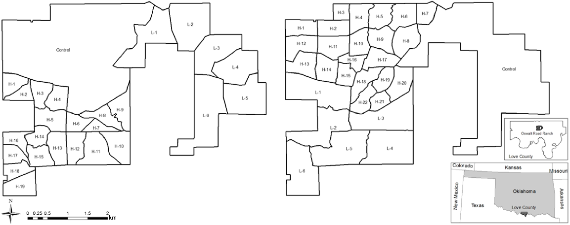
The Noble Research Institute’s Oswalt Road Ranch (ORR) is in Love County, Oklahoma, USA (Fig. 1). The ORR property is an 1861-ha ranch within the Cross Timbers and Prairie eco-region, consisting of mixed wooded areas, bottomlands, uplands and rangeland (Gee et al. 2011). To mitigate the carryover effect of previous hunting on the ORR, lease hunting (x̅ = 5 hunters) ceased after the 2006 hunting season. No hunting occurred on the ORR until our study began in 2008. Additionally, the ORR management team did not conduct any cattle grazing or prescribed fire management on the ranch during our study. Refer to Little et al. (2014) for additional study area details.
The Noble Research Institute’s Oswalt Road Ranch located in Love County, Oklahoma, USA, with treatment compartments delineated. Left: 2008 treatment compartments where control (C) = no hunters on 679 ha; low-risk (L) = 1 hunter/101 ha on 585 ha total; and high-risk (H) = 1 hunter/30 ha on 583 ha total. Right: compartments were shifted clockwise for the 2009 hunting season where control (C) = no hunters on 586 ha; low-risk (L) = 1 hunter/101 ha on 583 ha total; and high-risk (H) = 1 hunter/30 ha on 679 ha total. Map produced in ArcGIS 10.6.1 (ArcGIS® software by Esri).
Hunter assignment and observations
We divided the ORR into three treatment areas of similar size and vegetation composition based on existing landscape features, property boundaries, etc. (Little et al. 2014, 2016). These areas consisted of no hunting pressure (control), low hunting pressure (1 hunter/101 ha), and high hunting pressure (1 hunter/30 ha). We further divided the treatments into hunting compartments to maintain the proper hunter per hectare density for the different hunting pressures. The high hunting pressure treatment area was divided into 19 compartments in 2008 and 21 compartments in 2009, and the low hunting pressure treatment area was divided into six compartments both years. Individual hunters were assigned to one hunting compartment for that hunting period. For additional information on the study design, see Little et al. (2014, 2016).
Noble Research Institute employees collected hunt data and equipped hunters with GPS units to collect accurate and unbiased data on hunter behavior. Hunters were required to spend ≥4 h/day per compartment during the weekend when participation was highest. At all times, hunters carried a Garmin Etrex Venture GPS unit (Garmin, Olathe KS) to track their locations with a fix attempt every minute (recorded in datum NAD83, UTM Zone 14N, accuracy ±10 m). To remove locations not associated with hunting behavior, we truncated GPS location data to coincide with legal shooting hours and within assigned hunting compartments. Hunters were required to record the start and end times of their activities within the assigned hunting compartment each day, the number of deer observed within the compartment (number of collared antlered deer, and number of un-collared antlered and antlerless deer), and hunting method used (e.g. tree-stand, ground-blind, still, or specified other). For analytical purposes, we grouped hunting methods into the following three classes and report statistics for each class: still hunting (moving slowly and quietly through an area), stand hunting (using a tree stand or ground blind), and multiple methods (e.g. stalking then used tree-stand, scouting, etc.).
Landscape classification
The Noble Research Institute developed a vegetation type and land-use map combined with a digital elevation model (DEM). Digital raster layers were re-sampled using a 1 m resolution grid into a 17 m resolution grid following the 2009 growing-season National Agriculture Imagery Program (NAIP; USDA Farm Service Agency, Salt Lake City, UT, USA) aerial imagery and using ERDAS Imagine software (ver. 9.3; ERDAS, Inc., Atlanta, GA, USA; Little 2011). The following three vegetative cover types were classified on the basis of vegetation structure of the study area: forest, mixed communities consisting of any combination of forest, shrub, and grassland, but primarily shrub–grassland, and grassland. Refer to Little (2011) for additional landscape classification details.
Analytic approach
Movement covariates
We used Program R packages ‘trajr’ (ver. 1.3.0; https://github.com/JimMcL/trajr; McLean and Skowron Volponi 2018), ‘adehabitatLT’ (ver. 0.3.25; https://cran.r-project.org/web/packages/adehabitatLT/adehabitatLT.pdf; Calenge 2006), and ‘recurse’ (ver. 1.4.0; https://cran.r-project.org/web/packages/recurse/index.html; Bracis et al. 2018) to calculate movement parameters on the basis of GPS location data for each hunter during each recorded hunt. These movement parameters were divided into two suites of movement metric for analysis, namely, movement and path shape. To represent hunter movement, we calculated step length, net squared displacement, and residence time for each recorded hunt. Step length was the length (m) between two consecutive points in a trajectory (McLean and Skowron Volponi 2018). Net squared displacement (m2) was the square of the Euclidean distance between each point in the trajectory and the origin (i.e. first location) of the movement path (Bastille-Rousseau et al. 2015). Residence time was the total time spent (min) within a defined radius equal to the maximum standard GPS fix error (10 m + 3.6 s.e.; Bracis et al. 2018). Additionally, we calculated residence time as a proportion of the total time spent hunting to adjust for variation in hunt length. To represent path shape, we calculated the turning angle and sinuosity of each recorded hunt. Turning angle was the direction (radians) in which the hunter traveled between consecutive points in a trajectory (McLean and Skowron Volponi 2018). This was an absolute value to highlight the severity of the turn rather than the direction. Sinuosity was calculated using the standard deviation of the turning angle divided by the square root of the step length and is an index from 0 to 1 representing the straightness of a trajectory, where 0 is straight and 1 is highly curved (Bovet and Benhamou 1988). For each movement parameter, except sinuosity which is a scaled index, we calculated summary statistics for each hunt including the following values: minimum, median, maximum, mean, standard deviation, variance, and coefficient of variation.
Habitat-use covariates
Using both continuous and discrete data, hunter habitat use was divided into the following two suites: proportion of time spent in vegetation cover classes and the mean use of landscape features. Vegetation cover classes were represented using the landcover raster layer classes for forest, mixed, grassland, and riparian cover. We extracted raster cell values from GPS locations for each recorded hunt by using the ‘raster’ package (ver. 3.6-31; https://cran.r-project.org/web/packages/raster/index.html; Hijmans et al. 2015) in Program R. Habitat use was calculated by dividing the count of cells used for each vegetation cover class by the total number of GPS locations in each recorded hunt to create a value representing the proportion of locations spent in a vegetation cover class during a single hunt.
Use of landscape features was represented using distance to features and the roughness data layers created in ArcGIS (ver. 10.6.1; ArcGIS® software by Esri). We performed a reclassification of the landcover raster layer where each cell in the new raster layers was given a value based on the Euclidean distance from the specified feature. This included distance to anthropogenic features, ponds, and roads. Because there is less than 100 m of variation in elevation on ORR, we used roughness to represent variation in topography. The scale at which hunters perceive the landscape was considered the average shooting distance for the study area, which is 100–150 m (Springer 1977). Thus, to create the roughness layer, we used a 30 m resolution digital elevation model (DEM) raster layer and performed a zonal reclassification by using a 10 × 10 roving window to represent the shooting window (150 m × 150 m), where the standard deviation of the elevation was assigned to the focal cell. We then extracted raster cell values for GPS locations for each recorded hunt by using the ‘raster’ package (ver. 3.6-31; Hijmans et al. 2015) in Program R and took the mean value for distance to anthropogenic features, ponds, and roads, and the mean landscape roughness for each recorded hunt.
Population-level resource selection
To represent hunter habitat use at the population level, we examined all recorded hunts together. Hunters were assigned to specific compartments for the duration of the hunt, so we represented availability by creating one point per raster cell within the assigned compartment. Hunter presence was represented by the GPS location data. Resources available for use included vegetation cover classes and landscape features. We represented habitat covariates at the spatial scale at which hunters perceive the landscape, considered to be the average shooting distance of 150 m (Springer 1977). Using the landcover raster layer, we determined the dominant landcover class within the 150 m shooting window and assigned the focal cell accordingly. Landscape variation was represented as roughness by using the standard deviation of elevation. Raster cell values were extracted to each point by using the package ‘raster’ (ver. 3.6-31; Hijmans et al. 2015) in Program R.
Statistical analysis
Multistage modeling provides individual-based information on behaviors and links relationships among hunter habitat use, movement patterns, and observation rate of deer (Gillies et al. 2006; Dzialak et al. 2011; Wagner et al. 2011; Haus et al. 2020). To analyze the relative importance of covariates, we used a multi-stage modeling approach to reduce the number of competing models (Franklin et al. 2000). Covariates measuring related behavioral parameters were separated into suites, which included movement, path shape, vegetation cover class, and landscape features. We removed any covariates that were correlated (|r| ≥ 0.7) on the basis of Pearson’s correlation coefficient (Ranglack et al. 2017). We standardized all covariates by subtracting the mean and dividing by two times the standard deviation (Gelman 2008; Lele 2009). We evaluated multiple functional forms (linear, quadratic, and pseudothreshold) for each covariate as the relationship to observation rate could be non-linear. Pseudothreshold functional forms were fit by using a natural-log transformation (Franklin et al. 2000).
Our first stage of model selection for hunter behavior involved taking the individual behavioral suites and fitting univariate models for each covariate and functional form against the observation rate of white-tailed deer (deer observed per 1 h hunting; dependent variable) in competing models. To do this, we used a Gaussian distribution in a generalized linear model (GLM) by using the ‘lme4’ package in Program R (ver. 1.1-26; https://cran.r-project.org/web/packages/lme4/index.html; Bates et al. 2015). We then ranked the models using Akaike’s information criterion (AIC) (Akaike 2011) and moved all covariates within 2 ΔAIC units to the next stage of models (Ranglack et al. 2017). The second stage of model selection combined the most appropriate covariate functional forms within each suite to determine which covariate best represented movement and habitat use, resulting in the lowest AIC. The final stage model combined the best-performing models to represent both hunter movement and habitat-use behavior.
The multi-stage modeling process was replicated for the population level RSF, with only two stages of model selection. We separated covariates into two suites, namely, vegetation cover class and landscape features. The first-stage model selection fit univariate models for each hunter presence covariate and functional form in the two suites against resource availability in competing GLMs by using a binomial distribution. Including individual hunter as a random effect did not improve model fit (ΔAICc = 400510.5); therefore, random effects were not included and data were pooled by recorded hunt and not by individual, because some individuals hunted more than one outing. Models were ranked using AIC and all covariates within 2 ΔAICc units were moved to the next stage of models (Ranglack et al. 2017). The second stage of model selection combined the top covariate forms into a single model to represent hunter habitat use.
Numerous behavioral factors influence whether a hunter chooses to harvest an animal, thereby making it difficult to quantify and analyze. Thus, we used observation rate as a proxy for harvest success. To confirm the relationship between observation and harvest success, we performed binomial logistic regression analyses on the total number of deer observed and observation rate against harvest success (Little et al. 2014). Additionally, compartment availability of vegetation cover classes could have influenced hunter habitat use more strongly than hunter behavior. Thus, to determine whether hunters were using vegetation cover classes in higher proportions to availability, we performed GLMs using a Gaussian distribution comparing hunter use and compartment availability functional responses (Gillies et al. 2006).
Results
During the 2008 and 2009 hunting seasons, 83 individual hunters recorded deer observation and location data for 516 unique hunts, collecting >140,000 GPS locations. Between the two hunting seasons, 29 animals were harvested by hunters (2008: 1 male, 10 females; 2009: 4 males, 14 females). Of the 516 records collected for this study, 29 were removed from analysis with associated errors (e.g. GPS recording error, missing observation data, hunter behavior did not follow instruction parameters, e.g. spending <1 h afield, leaving the assigned compartment, or using horses or ATVs) for a total of 487 recorded hunts used for all analyses, resulting in 111,706 GPS locations used for analyses.
Across all hunting methods, hunters spent an average of 3.7 h (s.e. = 0.1 h) afield during each recorded hunt, traveled 2085 m (s.e. = 79.0 m), and observed 2.7 deer/hunt (s.e. = 0.15). Hunters primarily used still and stand hunting methods, with many hunters using a combination of methods. During each recorded hunt, hunters spent an average 3.7 h afield (s.e. = 0.1; 879 total h) for still hunting, 3.8 h (s.e. = 0.1; 1256 total h) for stand hunting, and 4.7 h (s.e. = 0.7; 52 total h) when using multiple methods. Overall, hunters observed 1336 deer (male: 303; female: 696; fawns: 194; and unknown: 143) with an average rate of observation for males (0.3/h, s.e. = 0.02), females (0.6/h, s.e. = 0.04), and fawns (0.2/h, s.e. = 0.02). Still hunters observed 0.9 deer/h (s.e. = 0.1), stand hunters observed 0.7 deer/h (s.e. = 0.05), and hunters using multiple methods observed 0.4 deer/h (s.e. = 0.2). Between each GPS fix (1 fix per min), the mean step length per recorded hunt averaged at 9.4 m (s.e. = 0.3) and the mean absolute turning angle of hunters per recorded hunt averaged 0.3 radians (s.e. = 0.01). Mean residence time averaged 46%, indicating that hunters spent 46% of their time within 10 m (±3.6 s.e.) of the previous GPS location. The percentage of use for different vegetation cover classes per hunt time averaged 16% forested cover (s.e. = 0.01), 22% mixed cover (s.e. = 0.01), and 38% grassland cover (s.e. = 0.02), and 24% riparian cover; topographic roughness averaged 5.8 (s.e. = 0.1; Table 1).
| Variable | Mean | s.e. | |
|---|---|---|---|
| Total observations (number of deer) | 2.74 | 0.15 | |
| Total time (h) | 3.73 | 0.08 | |
| Total distance (m) | 2085 | 79 | |
| Mean step length (m/min) | 9.41 | 0.30 | |
| Mean turning angle (radians) | 0.27 | 0.01 | |
| Residence time (proportion of hunt) | 0.46 | 0.01 | |
| Forest use (proportion of hunt) | 0.16 | 0.01 | |
| Mixed use (proportion of hunt) | 0.22 | 0.01 | |
| Grassland use (proportion of hunt) | 0.37 | 0.02 | |
| Mean roughness (s.d. of elevation) | 5.77 | 0.10 |
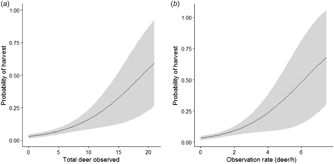
We confirmed the relationship between observation rate and harvest success. The probability of harvest increased as the total number of deer observed increased (P < 0.01, s.e. = 0.04, z = 4.398) and as observation rate increased (P < 0.01, s.e. = 0.14, z = 3.916) (Fig. 2).
Plots of binomial logistic regression models of white-tailed deer harvest by hunters. (a) Total deer observed during a hunt (number of deer); and (b) observation rate (number of deer/h).
Deer observation rates
From the GLMs, using a Gaussian distribution, the best covariates for each movement suite and functional form included linear mean step length, mean turning angle as a quadratic function, and mean residence time as a quadratic function (observed deer/h ~ mean step length + mean turning angle + mean turning angle2 + mean residence time + mean residence time2; Table 2). There were two models within 2 ΔAICc units of the top model for hunter movement; therefore, we selected the most parsimonious model. This model involved linear mean step length and mean turning angle as a quadratic function (observed deer/h ~ mean step length + mean turning angle + mean turning angle2).
| Covariate | Estimate | s.e. | t-value | P-value | |
|---|---|---|---|---|---|
| Intercept | 0.58 | 0.07 | 8.24 | <0.01 | |
| Mean step length | 0.35 | 0.14 | 2.55 | 0.01 | |
| Mean turning angle | 0.06 | 0.10 | 0.62 | 0.54 | |
| (Mean turning angle)2 | 0.31 | 0.12 | 2.66 | <0.01 | |
| Mean residence time | 0.01 | 0.14 | 0.06 | 0.95 | |
| (Mean residence time)2 | 0.52 | 0.20 | 2.59 | <0.01 |
The best covariates for each habitat use suite and functional form included linear proportion for use of grasslands, forests, mixed, and mean roughness (observed deer/h ~ proportion of hunt spent in grasslands + proportion of hunt spent in forests + proportion of hunt spent in mixed habitat + mean roughness; Table 3). Distance covariates did not show a significant effect on observation rate. There were five models within 2 ΔAICc units of the top model for hunter habitat use (Table 4); therefore, the most parsimonious model was selected, containing only the proportion of forested cover used (observed deer/h ~ proportion of hunt spent in forest).
| Covariate | Estimate | s.e. | t-value | P-value | |
|---|---|---|---|---|---|
| Intercept | 0.79 | 0.04 | 17.91 | <0.01 | |
| Proportion of grassland use | −0.04 | 0.1 | −0.42 | 0.67 | |
| Proportion of forest use | 0.4 | 0.1 | 3.79 | <0.01 | |
| Proportion of mixed use | 0.06 | 0.1 | 0.59 | 0.56 | |
| Mean roughness | 0.11 | 0.09 | 1.17 | 0.24 |
| Model | d.f. | logLik | ΔAICc | Weight | |
|---|---|---|---|---|---|
| Deer/h ~ forest | 3 | −674.82 | 0.00 | 0.26 | |
| Deer/h ~ forest + roughness | 4 | −674.08 | 0.55 | 0.19 | |
| Deer/h ~ forest + mixed | 4 | −674.43 | 1.25 | 0.14 | |
| Deer/h ~ forest + grassland | 4 | −674.53 | 1.45 | 0.12 | |
| Deer/h ~ forest + mixed + roughness | 5 | −673.72 | 1.89 | 0.10 |
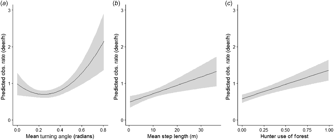
The top combined model for hunter movement and habitat use included all of the best competing covariates: linear mean step length, mean turning angle as a quadratic function, and linear proportion of hunt spent in forested cover (observed deer/h ~ mean step length + mean turning angle + mean turning angle2 + proportion of hunt spent in forested cover; Table 5). As average step length increased, the model predicted the number of deer observed per hour increased (standardized coefficient estimate ± s.e.; 0.3 ± 0.09; Fig. 3). The predicted number of deer observed was the lowest when the mean absolute turning angle was approximately 0.3 radians, with predicted observations increasing as the mean absolute turning angle increased, or approached 0 (0.06 ± 0.1; Fig. 3). As the mean proportion of hunt time spent within forested cover increased, the number of deer observed per hour increased (0.42 ± 0.09; Fig. 3).
| Covariate | Estimate | s.e. | P-value | t-value | |
|---|---|---|---|---|---|
| Intercept | 0.70 | 0.05 | <0.01 | 13.54 | |
| Mean step length | 0.30 | 0.09 | <0.01 | 3.16 | |
| Mean turning angle | 0.06 | 0.1 | 0.51 | 0.65 | |
| (Mean turning angle)2 | 0.34 | 0.1 | <0.01 | 3.01 | |
| Proportion of forest use | 0.42 | 0.09 | <0.01 | 4.83 |
Hunter use of landscape
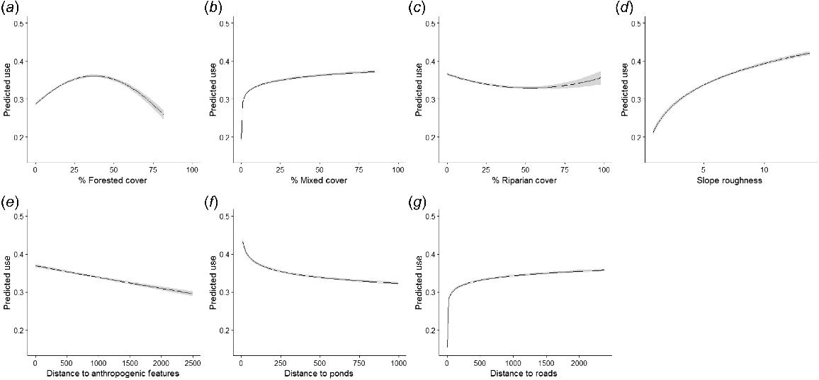
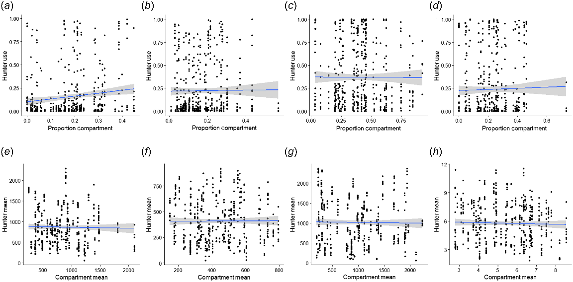
We found that the best competing functional forms for each covariate included in our hunter resource selection models included the following: distance to ponds and roads as pseudothresholds, linear distance to anthropogenic features, forest and riparian cover as quadratic functions, mixed cover as a pseudothreshold, and roughness as a pseudothreshold (Used ~ Log(distance to ponds ± 0.001) + Log(distance to roads + 0.001) + Distance to anthropogenic features + Forest cover + Forest cover2 + Riparian cover + Riparian cover2 + Log(mixed cover +0.001) + Log (roughness + 0.001); Table 6). The most supported model included each of the covariates (model weight = 1), with the next highest model within 41.21 ΔAICc units. Predicted hunter use of forested cover was greatest at 40% forested habitat within the shooting window (Fig. 4). Predicted hunter use of mixed cover quickly increased before reaching an asymptote at 5% mixed cover within the shooting window (Fig. 4). Predicted hunter use of riparian cover was lowest at 50% riparian cover within the shooting window, with use increasing as availability either increased or approached 0% (Fig. 4). Predicted hunter use decreased as distance to ponds increased, quickly reaching an asymptote in predicted use after approximately 200 m of distance (Fig. 4). Predicted hunter use increased as distance to roads increased, quickly reaching its threshold at approximately 50 m of distance (Fig. 4). Predicted hunter use increased as roughness increase, and distance to anthropogenic features increased (Fig. 4). Hunters showed greater use of forested cover in proportion to availability than other vegetation cover classes (P < 0.01, s.e. = 0.10, t = 3.227; Fig. 5).
| Covariate | Estimate | s.e. | P-value | z-value | |
|---|---|---|---|---|---|
| Intercept | −0.78 | 0.01 | <0.01 | −119.96 | |
| Distance to anthropogenic features | −0.12 | 0.01 | <0.01 | −8.72 | |
| Log(distance to ponds) | −0.22 | 0.01 | <0.01 | −32.99 | |
| Log(distance to roads) | 0.26 | 0.01 | <0.01 | 26.13 | |
| Forested habitat | 0.31 | 0.01 | <0.01 | 26.99 | |
| (Forested habitat)2 | −0.31 | 0.01 | <0.01 | −21.96 | |
| Log(mixed habitat) | 0.43 | 0.01 | <0.01 | 43.58 | |
| Riparian habitat | −0.16 | 0.01 | <0.01 | −16.61 | |
| (Riparian habitat)2 | 0.11 | 0.02 | <0.01 | 5.97 | |
| Log(roughness) | 0.34 | 0.01 | <0.01 | 34.50 |
Plots of seven covariates included in the top model of population level resource selection of white-tailed deer hunters. (a) Percentage forested cover of shooting window; (b) percentage mixed cover of shooting window; (c) percentage riparian cover of shooting window; (d) available roughness (s.d. of elevation); (e) available distance to anthropogenic features (m); (f) available distance to ponds (m); and (g) available distance to roads (m).
Functional response of hunter use versus compartment availability. (a) Proportion of hunter use of forested habitat over proportion of forested habitat available within a compartment; (b) proportion of hunter use of mixed habitat over proportion of mixed habitat available within a compartment; (c) proportion of hunter use of grassland habitat over proportion of grassland habitat available within a compartment; (d) proportion of hunter use of riparian habitat over proportion of riparian habitat available within a compartment; (e) mean hunter distance from anthropogenic features (m) over mean compartment distance from anthropogenic features (m); (f) mean hunter distance from ponds (m) over mean compartment distance from ponds (m); (g) mean hunter distance from roads (m) over mean compartment distance from roads (m); and (h) mean hunter roughness (s.d. of elevation) over mean compartment roughness (s.d. of elevation).
Discussion
Most research has focused on the effect of hunting pressure on prey behavior, whereas little research has analyzed hunter behavior and its potential effects on harvest success. Hunter behavior, in terms of how movement and habitat use influence observation of deer, has not been previously measured on such a fine temporal and spatial scale. Our results suggest that hunter movement and habitat use influenced the number of deer observed during a hunt. Hunters that used forested cover in greater proportions were more likely to observe deer than were hunters that used forested cover in lesser proportions. Additionally, hunters selected mixed cover more consistently than forested cover, relative to availability. Hunters with greater movement rates were more likely to observe deer than were hunters with lower rates of movement. Walking at approximately 25 m/min (1 mph), the model predicts that hunters will observe one deer per hour. During movement, hunters that either did not turn or turned more sharply were more likely to observe deer than were hunters that turned more moderately, suggesting that decisive, directional movements may increase likelihood of observation. However, it is important to note that not every observation results in a harvest opportunity (e.g. observing a fleeing animal). Although the probability of harvest generally increases with higher observation rates, this is highly dependent on the specific scenario (Fig. 2). For instance, a hunter may observe more deer, but they could simply be fleeing, which does not guarantee an increased harvest rate.
Previous research found that hunter effort and observation rate were dependent on road access, landscape features, visibility, prey densities, and experience (Jacques et al. 2011; Lebel et al. 2012; Norum et al. 2015; Ranglack et al. 2017; O’Connor et al. 2018), and prey altered their vigilance behaviors, movement patterns, and habitat use (Kufeld et al. 1988; Kilgo et al. 1998; Conner et al. 2001; Stankowich 2008; Bonnot et al. 2013; Little et al. 2016; Marantz et al. 2016). In response to hunting pressure, some ungulates increased selection for areas of greater cover (Kufeld et al. 1988; Kilgo et al. 1998; Bonnot et al. 2013; Lone et al. 2015; Ranglack et al. 2017), whereas some selected for more open habitats with greater visibility within flight distance to cover (Swenson 1982; Stankowich 2008). Prey distribution changed over the hunting season as prey increased awareness of predation risk and altered movement and behavior (Little et al. 2014); for example, prey species become more vigilant and are more likely to flee when there is a perceived risk (Frid and Dill 2002; Stankowich 2008; Schuttler et al. 2017). During the study period, deer avoided hunting pressure by increasing selection for forested cover (Little 2011), decreasing diurnal movement (Little et al. 2016), and increasing site fidelity (Marantz et al. 2016). Deer increased use of forested cover by 1.7–2.5 times and mixed cover by 1.4–2.3 times in response to predation pressure (Little 2011). Collared deer that were unobserved by hunters moved 38.3% less than did observed collared deer, suggesting that greater movement increased observability (Little 2011).
We observed a positive relationship between the number of deer observed and harvest success, which supports our use of observation rate as a proxy to harvest success. Although, it is important to consider that increased observations do not necessarily equate to increased harvest in all cases, because hunters may simply be observing a moving deer that cannot be ethically and legally harvested, or they choose not to harvest the specific animal. For the 2008 and 2009 hunting seasons, ORR had a harvest quota of 20 antlerless deer each year, with three mature, un-collared antlered deer in 2008, and four mature, un-collared antlered deer in 2009. This showed limited harvest on the property, while observations were unlimited. Only 29 harvests occurred during the study period, whereas 1333 deer were observed, leading to the relationship being highly variable. Further research, with higher rates of harvest success, is necessary to more confidently determine the strength of the relationship between observation of prey and likelihood of harvest.
Given that deer increase their use of concealment cover at the onset of the hunting season (Swenson 1982; Kufeld et al. 1988; Kilgo et al. 1998; Paton et al. 2017), visual obstruction can be a determining factor in harvest success (Lone et al. 2015). However, our results showed that as deer increase the use of forested cover and decrease movement, hunters that increase the use of forested cover and increase movement are more likely to observe a deer by overlapping habitat use and potentially triggering a flight response (Grau and Grau 1980; Little et al. 2014, 2016). Prey perceive higher rates of movement and more direct trajectories as more threatening, triggering flight behavior (Grau and Grau 1980). As flight behavior is attention-attracting, deer that had greater movement during the hunting period were considered more observable (Little et al. 2014). Thus, the increased probability of observing deer as mean step length and mean absolute turning angle increased may be a result of triggering flight behavior in deer.
Interestingly, our results contradicted previous studies that have showed increased visibility to be a main indicator of harvest success (Swenson 1982; Jacques et al. 2011; Lebel et al. 2012; Plante et al. 2017). On ORR, visual obstruction increased from grasslands to forests (Little 2011), which should indicate a decrease in observation rate for hunters that used more forested cover, although this is dependant on deer density. The RSF determined that the predicted use of forested habitat was highest at 40% forested habitat within the shooting window of 150 m, with decreased predicted use as availability increased, whereas predicted use of mixed habitat reached a plateau after 5% mixed habitat within the shooting window (Fig. 4). This suggests that hunters selected mixed habitat when available more reliably than they did forested habitat. Mixed habitat had less visual obstruction than forested habitat, which may account for the selection of larger areas of mixed habitat, but this selection did not significantly affect observation rate. Deer altered their habitat use and movement behaviors following the initial 3-day exposure to predation pressure and selected more strongly for forested habitat than mixed habitat (Little 2011), suggesting that once deer are aware of predation pressure, overlapping habitat use becomes a more important factor in determining observation success than is visibility, because deer alter their movement and resource selection behaviors to avoid risk but learn to adapt their behaviors to avoid harvest (Little et al. 2014, 2016; Marantz et al. 2016).
Access roads have been shown to be a large influence on the number of hunting days per harvest, with hunters selecting for shorter distances from roads (Kilgo et al. 1998; Ranglack et al. 2017), which our data did not reflect. The RSF determined that predicted use increased as distance to roads increased (Fig. 4). However, this relationship did not show a significant effect on observation rate. Previous research has illustrated that most hunters focus their activity within as little as 100 m of a road or trail (Diefenbach et al. 2005; Lebel et al. 2012; Rowland et al. 2021). Thus, the probability of harvest generally increases as the amount of access roads increases within hunting areas, dependent on the degree of visibility, traffic and density of roads (Lebel et al. 2012; Paton et al. 2017; Plante et al. 2017; O’Connor et al. 2018). ORR did not have substantive internal road systems for hunters to utilize during their hunts. Compartment boundaries were often marked by pathways and simple, two-track roads, which limited hunter use as well. Additionally, the truncation of movement to be within assigned compartments removed nearly all use of roads by eliminating transit to and from the compartment. Although roads may be a significant source of hunter decision on other properties and within other studies (Kilgo et al. 1998; Gratson and Whitman 2000; Ranglack et al. 2017), the layout of ORR and the study design largely eliminated the use of roads by hunters. Our findings reflect this, because we did not find a significant effect on observation rate. Hunters also showed a strong preference in their selection of areas with higher roughness (Fig. 4), which aligns with literature suggesting varying topography to be an indicator of success (Swenson 1982; Iijima 2017). However, the low variation of the topography of the study area led to no significant effect of roughness on observation rate of deer. Given that the elevation of the study area ranged from 233 to 300 m and the slope averaged 4.12 degrees (s.e. = 0.02) (S. Webb, unpubl. data), habitat composition had a greater effect on visibility than topography in terms of observation rate.
It is important to note that hunters participating in this study were limited in their decision-making options regarding behavioral choices. Because this study was originally designed to control for hunting pressure across a landscape by assigning hunters to compartments (Little 2011), hunters were limited to what was available to them within the compartment. Compartments could vary greatly in habitat composition and landscape features. Coupled with the truncation of GPS location points, this could account for the sharp threshold reached in predicted use as distance to ponds and roads increased, as well as the negative linear relationship of distance to anthropogenic features in the RSF. The available riparian cover ranged from 0 to 73%, with an average of 22% of the compartment composition. Despite the high variability of available riparian habitat, predicted use of riparian cover varied only from 0.33 to 0.38 (Fig. 4), suggesting that hunters did not select strongly for riparian areas and this selection did not have a significant effect on observation rate. The available forested cover ranged from 0 to 45%, with an average of 18% of the compartment composition; however, hunters used forested cover in higher proportions to compartment availability (Fig. 5). Given that use of forested habitat was one of the most important covariates in predicting the number of deer observed, hunters that had limited availability of forested cover at their disposal during their hunts did not necessarily observe less deer because of active behavioral decisions, but rather because of predetermined compartment.
However, our results are context dependent, with an 18% average forest cover in our hunting compartments, compared with states in eastern United States that are predominantly forested. Therefore, future research should continue to explore this relationship between deer-hunters and land-use patterns.
Management implications
One issue currently facing management agencies is the low recruitment and retention of hunters (Ryan and Shaw 2011). Hunting is an activity based long in tradition, with methods and locations passed down through the generations (Gratson and Whitman 2000) and, often, knowledge can be a barrier to new hunters in an area (Ryan and Shaw 2011). Additionally, hunter satisfaction is linked with harvest success, which influences hunter opinion of management efforts by agencies (Miller and Graefe 2001). Therefore, providing hunters with behavioral tools to increase the likelihood of harvest success increases hunter satisfaction in agency management of wildlife while also maintaining hunting as a viable management tool.
White-tailed deer populations are increasing throughout their range across the United States (Urbanek et al. 2011), and urbanization and habitat fragmentation have pushed deer into more conflict with humans (Green et al. 1997; Kilpatrick et al. 2007; Urbanek et al. 2011). There is a growing need to improve hunting as a management tool to more effectively manage growing populations (Cromsigt et al. 2013). By identifying and optimizing where hunter and prey behaviors interact, managers have the potential to create more targeted approaches to hunting and population management. The ability to determine what behaviors and areas maximize the probability of harvest, for example, movement through forested cover, may increase the efficiency and effectiveness of hunting as a tool. In the case of urban and suburban deer management where agencies must consider how to remove a specific number of animals from an area with limited time and space availability (Hansen and Beringer 1997; Kilpatrick and Walter 1999; Kilpatrick et al. 2002, 2007), the ability to maximize probability of behavioral overlaps between deer and hunters could increase the efficiency of a targeted hunt. Our observations made during a highly regulated hunt on private property could also be of use to private landowners seeking to more effectively manage populations on their properties. Local wildlife agencies and private landowners can more strategically plan hunts on the basis of habitat composition of the property to meet management goals. Conversely, if the goal of management is to increase prey populations by decreasing harvest success, identifying what hunter behaviors lead to greater harvest success would delineate methods that could decrease the level of hunter harvest. Limiting the overlaps of habitat use by increasing road closures or adjusting hunting areas would likely decrease hunter success by limiting where hunter behaviors and prey behaviors overlap (Kilgo et al. 1998; Ranglack et al. 2017).
Declaration of funding
Funding was provided by Noble Research Institute, LLC (formerly The Samuel Roberts Noble Foundation, Inc.), the Department of Wildlife, Fisheries, and Aquaculture at Mississippi State University, and the University of Nebraska – Competitive Research Initiative. The funders had no role in the preparation of the data or the paper, or the decision to submit for publication.
Acknowledgements
This paper forms part of the Masters thesis of Alyssa Meier (2021). A. Meier was supported by an assistantship provided by University of Nebraska – Competitive Research Initiative. We thank Noble Research Institute for access to the property; all volunteers and hunters; R. Stevens, D. Payne, K. M. Webb, and F. Motal for technical and field assistance, and reviewers for improving early drafts of this paper. Thanks to Colorado Parks and Wildlife for making this article available Open Access.
References
Akaike H (2011) Akaike’s information criterion. In ‘International encyclopedia of statistical science’. (Ed. M Lovric) p. 25. (Springer: Berlin, Heidelberg, Germany). 10.1007/978-3-642-04898-2_110
Bastille-Rousseau G, Potts JR, Yackulic CB, Frair JL, Hance Ellington E, Blake S (2015) Flexible characterization of animal movement pattern using net squared displacement and a latent state model. Movement Ecology 4(1), 15.
| Crossref | Google Scholar |
Bates D, Mächler M, Bolker B, Walker S (2015) Fitting linear mixed-effects models using lme4. Journal of Statistical Software 67(1), 1-48.
| Crossref | Google Scholar |
Bonnot N, Morellet N, Verheyden H, Cargnelutti B, Lourtet B, Klein F, Hewison AJM (2013) Habitat use under predation risk: hunting, roads and human dwellings influence the spatial behaviour of roe deer. European Journal of Wildlife Research 59(2), 185-193.
| Crossref | Google Scholar |
Bovet P, Benhamou S (1988) Spatial analysis of animals’ movements using a correlated random walk model. Journal of Theoretical Biology 131(4), 419-433.
| Google Scholar |
Bracis C, Bildstein KL, Mueller T (2018) Revisitation analysis uncovers spatio-temporal patterns in animal movement data. Ecography 41(11), 1801-1811.
| Crossref | Google Scholar |
Calenge C (2006) The package ‘adehabitat’ for the R software: a tool for the analysis of space and habitat use by animals. Ecological Modelling 197(3–4), 516-519.
| Crossref | Google Scholar |
Conner MM, White GC, Freddy DJ (2001) Elk movement in response to early-season hunting in Northwest Colorado. Journal of Wildlife Management 65(4), 926-940.
| Crossref | Google Scholar |
Cromsigt JPGM, Kuijper DPJ, Adam M, Beschta RL, Churski M, Eycott A, Kerley GIH, Mysterud A, Schmidt K, West K (2013) Hunting for fear: innovating management of human–wildlife conflicts. Journal of Applied Ecology 50(3), 544-549.
| Crossref | Google Scholar |
Diefenbach DR, Finley JC, Luloff AE, Stedman R, Swope CB, Zinn HC, San Julian GJ (2005) Bear and deer hunter density and distribution on public land in Pennsylvania. Human Dimensions of Wildlife 10(3), 201-212.
| Crossref | Google Scholar |
Doerr ML, McAninch JB, Wiggers EP (2001) Comparison of 4 methods to reduce white-tailed deer abundance in an urban community. Wildlife Society Bulletin 29(4), 1105-1113.
| Crossref | Google Scholar |
Dzialak MR, Webb SL, Harju SM, Winstead JB, Wondzell JJ, Mudd JP, Hayden-Wing LD (2011) The spatial pattern of demographic performance as a component of sustainable landscape management and planning. Landscape Ecology 26(6), 775-790.
| Crossref | Google Scholar |
Franklin AB, Anderson DR, Gutiérrez RJ, Burnham KP (2000) Climate, habitat quality, and fitness in northern spotted owl populations in northwestern California. Ecological Monographs 70(4), 539-590.
| Crossref | Google Scholar |
Frid A, Dill L (2002) Human-caused disturbance stimuli as a form of predation risk. Ecology and Society 6(1), 11.
| Google Scholar |
Gelman A (2008) Scaling regression inputs by dividing by two standard deviations. Statistics in Medicine 27, 2865-2873.
| Crossref | Google Scholar | PubMed |
Gillies CS, Hebblewhite M, Nielsen SE, Krawchuk MA, Aldridge CL, Frair JL, Saher DJ, Stevens CE, Jerde CL (2006) Application of random effects to the study of resource selection by animals. Journal of Animal Ecology 75(4), 887-898.
| Crossref | Google Scholar | PubMed |
Gratson MW, Whitman C (2000) Characteristics of Idaho elk hunters relative to road access on public lands. Wildlife Society Bulletin 28(4), 1016-1022.
| Google Scholar |
Grau GA, Grau BL (1980) Effects of hunting on hunter effort and white-tailed deer behavior. Ohio Journal of Science 80(4), 150-156.
| Google Scholar |
Green D, Askins GR, West PD (1997) Developing urban deer management plans: the need for public education. In ‘Proceedings of the Eighth Eastern Wildlife Damage Management Conference’, 16–19 October 1997, Roanoke, Virginia. (Ed. JA Parkhurst) pp. 95–103. Available at https://digitalcommons.unl.edu/ewdcc8/15
Hansen L, Beringer J (1997) Managed hunts to control white-tailed deer populations on urban public areas in Missouri. Wildlife Society Bulletin 25(2), 484-487.
| Google Scholar |
Harden CD, Woolf A, Roseberry J (2005) Influence of exurban development on hunting opportunity, hunter distribution, and harvest efficiency of white-tailed deer. Wildlife Society Bulletin 33(1), 233-242.
| Crossref | Google Scholar |
Haus JM, Webb SL, Strickland BK, McCarthy KP, Rogerson JE, Bowman JL (2020) Individual heterogeneity in resource selection has implications for mortality risk in white-tailed deer. Ecosphere 11(4), e03064.
| Crossref | Google Scholar |
Hijmans RJ, Van Etten J, Cheng J, Mattiuzzi M, Sumner M, Greenberg JA, Lamigueiro OP, Bevan A, Racine EB, Shortridge A, Hijmans MR (2015) Package ‘raster’. R package 734, 473.
| Google Scholar |
Hygnstrom SE, Vercauteren KC, Groepper SR, Garabrandt GW, Gubanyi JA (2011) Effects of seasons and hunting on space use by female white-tailed deer in a developed landscape in southeastern Nebraska. Wildlife Society Bulletin 35(3), 220-226.
| Crossref | Google Scholar |
Iijima H (2017) The effects of landscape components, wildlife behavior and hunting methods on hunter effort and hunting efficiency of sika deer. Wildlife Biology 2017(1), 1-6.
| Crossref | Google Scholar |
Jacques CN, van Deelen TR, Hall WH, Jr., Martin KJ, Vercauteren KC (2011) Evaluating how hunters see and react to telemetry collars on white-tailed deer. Journal of Wildlife Management 75(1), 221-231.
| Crossref | Google Scholar |
Johnson-Bice SM, Gable TD, Homkes AT, Windels SK, Bump JK, Bruggink JG (2023) Logging, linear features, and human infrastructure shape the spatial dynamics of wolf predation on an ungulate neonate. Ecological Applications 33(7), e2911.
| Crossref | Google Scholar |
Kilgo JC, Labisky RF, Fritzen DE (1998) Influences of hunting on the behavior of white-tailed deer: implications for conservation of the Florida panther. Conservation Biology 12(6), 1359-1364.
| Google Scholar |
Kilpatrick HJ, Walter WD (1999) A controlled archery deer hunt in a residential community: cost, effectiveness, and deer recovery rates. Wildlife Society Bulletin 27(1), 115-123.
| Google Scholar |
Kilpatrick HJ, Spohr SM, Chasko GG (1997) A controlled deer hunt on a state-owned coastal reserve in Connecticut: controversies, strategies, and results. Wildlife Society Bulletin 25(2), 451-456.
| Google Scholar |
Kilpatrick HJ, LaBonte AM, Seymour JT (2002) A shotgun-archery deer hunt in a residential community: evaluation of hunt strategies and effectiveness. Wildlife Society Bulletin 30(2), 478-486.
| Google Scholar |
Kilpatrick HJ, LaBonte AM, Barclay JS (2007) Acceptance of deer management strategies by suburban homeowners and bowhunters. Journal of Wildlife Management 71(6), 2095-2101.
| Crossref | Google Scholar |
Kufeld RC, Bowden DC, Schrupp DL (1988) Influence of hunting on movements of female mule deer. Journal of Range Management 41(1), 70-72.
| Crossref | Google Scholar |
Laliberte AS, Ripple WJ (2004) Range contractions of North American Carnivores and Ungulates. BioScience 54(2), 123-138.
| Crossref | Google Scholar |
Lebel F, Dussault C, Massé A, Côté SD (2012) Influence of habitat features and hunter behavior on white-tailed deer harvest. Journal of Wildlife Management 76(7), 1431-1440.
| Crossref | Google Scholar |
Lele SR (2009) A new method for estimation of resource selection probability function. Journal of Wildlife Management 73(1), 122-127.
| Crossref | Google Scholar |
Little AR, Demarais S, Gee KL, Webb SL, Riffell SK, Gaskamp JA, Belant JL (2014) Does human predation risk affect harvest susceptibility of white-tailed deer during hunting season? Wildlife Society Bulletin 38(4), 797-805.
| Crossref | Google Scholar |
Little AR, Webb SL, Demarais S, Gee KL, Riffell SK, Gaskamp JA (2016) Hunting intensity alters movement behaviour of white-tailed deer. Basic and Applied Ecology 17(4), 360-369.
| Crossref | Google Scholar |
Lone K, Loe LE, Meisingset EL, Stamnes I, Mysterud A (2015) An adaptive behavioural response to hunting: surviving male red deer shift habitat at the onset of the hunting season. Animal Behaviour 102, 127-138.
| Crossref | Google Scholar |
Marantz SA, Long JA, Webb SL, Gee KL, Little AR, Demarais S (2016) Impacts of human hunting on spatial behavior of white-tailed deer (Odocoileus virginianus). Canadian Journal of Zoology 94(12), 853-861.
| Crossref | Google Scholar |
McGhee KE, Pintor LM, Bell AM (2013) Reciprocal behavioral plasticity and behavioral types during predator–prey interactions. The American Naturalist 182(6), 704-717.
| Crossref | Google Scholar | PubMed |
McLean DJ, Skowron Volponi MA (2018) trajr: an R package for characterisation of animal trajectories. Ethology 124(6), 440-448.
| Crossref | Google Scholar |
Meier AN (2021) Effects of hunter movement and habitat use on observation rate of white-tailed deer (Odocoileus viginianus). Masters thesis. University of Nebraska at Kearney. Available at https://openspaces.unk.edu/bio-etd/4
Miller CA, Graefe AR (2001) Effect of harvest success on hunter attitudes toward white-tailed deer management in pennsylvania. Human Dimensions of Wildlife 6(3), 189-203.
| Crossref | Google Scholar |
Montgomery RA, Raupp J, Miller SA, Wijers M, Lisowsky R, Comar A, Bugir CK, Hayward MW (2022) The hunting modes of human predation and potential nonconsumptive effects on animal populations. Biological Conservation 265, 109398.
| Crossref | Google Scholar |
Murphy DA (1965) Effects of various opening days on deer. Proceedings of the Annual Conference, Southeastern Association of Game and Fish Commissioners 19, 141-146.
| Google Scholar |
Norum JK, Lone K, Linnell JDC, Odden J, Loe LE, Mysterud A (2015) Landscape of risk to roe deer imposed by lynx and different human hunting tactics. European Journal of Wildlife Research 61(6), 831-840.
| Crossref | Google Scholar |
O’Connor BJ, Fryda NJ, Ranglack DH (2018) Effects of environmental and anthropogenic landscape features on mule deer harvest in Nebraska. PeerJ 6(1), e5510.
| Crossref | Google Scholar |
Paton DG, Ciuti S, Quinn M, Boyce MS (2017) Hunting exacerbates the response to human disturbance in large herbivores while migrating through a road network. Ecosphere 8(6), e01841.
| Crossref | Google Scholar |
Plante S, Dussault C, Côté SD (2017) Landscape attributes explain migratory caribou vulnerability to sport hunting. Journal of Wildlife Management 81(2), 238-247.
| Crossref | Google Scholar |
Ranglack DH, Proffitt KM, Canfield JE, Gude JA, Rotella J, Garrott RA (2017) Security areas for elk during archery and rifle hunting seasons. Journal of Wildlife Management 81(5), 778-791.
| Crossref | Google Scholar |
Rowland MM, Nielson RM, Wisdom MJ, Johnson BK, Findholt S, Clark D, Didonato GT, Hafer JM, Naylor BJ (2021) Influence of landscape characteristics on hunter space use and success. Journal of Wildlife Management 85(7), 1394-1409.
| Crossref | Google Scholar |
Rowland MM, Nielson RM, Wisdom MJ, Clark DA, DiDonato GT, Hafer JM, Naylor BJ, Johnson BK (2023) Success is dependent on effort: unraveling characteristics of successful deer and elk hunters. Wildlife Society Bulletin 47(2), e1414.
| Crossref | Google Scholar |
Ryan EL, Shaw B (2011) Improving hunter recruitment and retention. Human Dimensions of Wildlife 16(5), 311-317.
| Crossref | Google Scholar |
Schuttler SG, Parsons AW, Forrester TD, Baker MC, McShea WJ, Costello R, Kays R (2017) Deer on the lookout: how hunting, hiking and coyotes affect white-tailed deer vigilance. Journal of Zoology 301(4), 320-327.
| Crossref | Google Scholar |
Stankowich T (2008) Ungulate flight responses to human disturbance: a review and meta-analysis. Biological Conservation 141(9), 2159-2173.
| Crossref | Google Scholar |
Swenson JE (1982) Effects of hunting on habitat use by mule deer on mixed-grass prairie in Montana. Wildlife Society Bulletin 10(2), 115-120.
| Google Scholar |
Urbanek RE, Allen KR, Nielsen CK (2011) Urban and suburban deer management by state wildlife-conservation agencies. Wildlife Society Bulletin 35(3), 310-315.
| Crossref | Google Scholar |
Wagner T, Diefenbach DR, Christensen SA, Norton AS (2011) Using multilevel models to quantify heterogeneity in resource selection. Journal of Wildlife Management 75(8), 1788-1796.
| Crossref | Google Scholar |