

Individual tree detection and classification from RGB satellite imagery with applications to wildfire fuel mapping and exposure assessments
L. Bennett A , Z. Yu A , R. Wasowski A , S. Selland A , S. Otway B and J. Boisvert A *
A
B
Abstract
Wildfire fuels are commonly mapped via manual interpretation of aerial photos. Alternatively, RGB satellite imagery offers data across large spatial extents. A method of individual tree detection and classification is developed with implications to fuel mapping and community wildfire exposure assessments.
Convolutional neural networks are trained using a novel generational training process to detect trees in 0.50 m/px RGB imagery collected in Rocky Mountain and Boreal natural regions in Alberta, Canada by Pleiades-1 and WorldView-2 satellites. The workflow classifies detected trees as ‘green-in-winter’/‘brown-in-winter’, a proxy for coniferous/deciduous, respectively.
A k-fold testing procedure compares algorithm detections to manual tree identification densities reaching an R2 of 0.82. The generational training process increased achieved R2 by 0.23. To assess classification accuracy, satellite detections are compared to manual annotations of 2 cm/px drone imagery resulting in average F1 scores of 0.85 and 0.82 for coniferous and deciduous trees respectively. The use of model outputs in tree density mapping and community-scale wildfire exposure assessments is demonstrated.
The proposed workflow automates fine-scale overstorey tree mapping anywhere seasonal (winter and summer) 0.50 m/px RGB satellite imagery exists. Further development could enable the extraction of additional properties to inform a more complete fuel map.
Keywords: communities, community protection, machine learning, planning, remote sensing, satellite imagery, trees, wildfire, wildfire fuels, wildfire preplanning, wildland-urban interface.
Introduction
Current wildfire science applications and exposure assessments require spatial maps of fuel types and fuel characteristics (Beverly et al. 2010; Tymstra et al. 2010; Linn et al. 2020). Fuel maps in Alberta, Canada are commonly derived from the Alberta Vegetation Inventory (AVI), a spatial dataset consisting of tree stand characteristics generated via the manual interpretation of aerial imagery by trained technicians (Frederick 2012; Forest Stewardship and Trade Branch 2022). Remote sensing allows for the collection of data over large spatial extents and provides an alternative to manual interpretation. Satellite imagery is widely available, and existing constellations regularly capture high spatial resolution imagery across large areas. For example, WorldView-2 captures panchromatic imagery at resolutions of up to 0.46 m with revisit times of up to 1.1 days, and Pleiades captures 0.50 m panchromatic imagery with daily revisit capacities (DigitalGlobe 2009; Airbus Defense and Space Intelligence 2012). Opportunity exists to leverage satellite imagery for the detection and classification of individual trees, which can then potentially inform community exposure.
Mapping wildfire fuels and assessing community exposure
Wildfire behaviour can be said to be governed by three factors: (1) weather; (2) topography; and (3) fuels. This is referred to as the ‘wildfire behaviour triangle’ because the three factors interact and drive wildfire behaviour (Countryman 1972). Of these three factors, only fuel can be realistically modified by humans. Quantifying fuel is a difficult task. Fuel properties can vary on a small spatial scale, but information about those properties is required across large spatial extents; Brandt et al. (2013) estimated the boreal zone covers 552 million ha in Canada, and Johnston and Flannigan (2018) estimated 32.3 million ha of wildland–urban interface (WUI), which are the areas where wildlands and the built environment meet. Here, focus is placed on ‘crown fuels’ as crown fires are high intensity fires that generate significant embers when accompanied by high winds (Van Wagner 1983). Embers are of particular interest; previous post-wildfire investigations have shown that the majority of structure ignitions are caused by ember exposure (Westhaver 2017). In Canada, crown fires are generally exclusive to coniferous forests, which burn with high intensity when compared to their deciduous counterparts (Van Wagner 1977). Thus, maps of coniferous and deciduous trees are helpful to quantify wildfire exposure and predict wildfire spread.
In Canada, the Fire Behaviour Prediction (FBP) system defines five groups of 16 fuel types (coniferous, deciduous, mixed-wood, slash, and open fuels) (Forestry Canada Fire Danger Group 1992). Fuel maps are utilised when predicting wildfire behaviour and assessing community exposure to wildfire, which can in turn be used for planning fuel reduction treatments, creating firelines/firebreaks along vulnerable parts of the WUI, and prioritising individual structures for risk reduction (Beverly et al. 2018).
Across Canada, the Canadian Forest Fire Danger Rating Systems (CFFDRS) is used as a consistent measure of fire danger, behaviour potential, and occurrence (Stocks et al. 1989). This system, which has been continually developed since 1968, has been the subject of a recent update that aims to be completed in 2025 (Canadian Forest Service Fire Danger Group 2021). CFFDRS-2025 includes the goal of having maps of a number of fuel structure attributes including tree species, diameter, height, proportion coniferous/deciduous, canopy closure, and density, and notes that many of these attributes have the potential to be mapped using remote sensing technologies (Canadian Forest Service Fire Danger Group 2021).
At a community scale, it is of interest to assess exposure to three wildfire ignition vectors: (1) radiant heat; (2) short-range firebrands; and (3) long-range firebrands. Assessments at this scale can enable prioritisation of mitigation activities and home-scale assessments and can allow for comparisons between communities (Beverly et al. 2010). Originally developed by Beverly et al. (2010), FireSmart Alberta defines a community exposure assessment procedure (Beverly et al. 2018). The assessment procedure requires hazard fuels to be mapped around the community. Depending on the ignition vector, the definition of hazard fuels described by Beverly et al. (2010) includes ‘FBP fuel types C-1 (spruce–lichen woodland), C-2 (boreal spruce), C-3 (mature jack or lodgepole pine), C-4 (immature jack or lodgepole pine), C-7 (ponderosa pine–Douglas-fir), O-1 (grass), and M-2 (boreal mixed-wood)’. Further, depending on the time of year and moisture content, certain fuels types such as aspen could be considered hazardous (Beverly et al. 2018). Once fuels are mapped, the community is divided into a grid. A moving circular window is used to calculate the area proportion of hazard fuel within the window at each grid cell. Three radii are used for the window, corresponding to different ignition types: (1) 30 m is used to assess for exposure to radiant heat from wildfires; (2) 100 m is used for short-range ember spotting; and (3) 100–500 m is used to assess exposure to longer range spotting (Beverly et al. 2010). The proportions of hazard fuel for each fuel type are then binned into nil, low, moderate, high, or extreme exposures. These exposure maps are useful for several reasons. As mentioned, ember exposure has been shown to be the primary reason for structure loss in previous WUI fire events in Alberta (Westhaver 2017). Thus, understanding where the community is most vulnerable to this ignition vector is key to pre-planning. Further, it has been shown that wildfires primarily occur in areas with high exposure to hazardous fuels (Beverly et al. 2021).
In Beverly et al. (2021), fuel maps were derived at a 100-m resolution using a combination of Alberta Vegetation Inventory (updated every 10–15 years), Alberta Ground Cover Characterisation (generated with satellite data from 2000) (Sanchez-Azofeifa et al. 2004), and annually updated disturbance inventories. In Beverly et al. (2010), land cover and structures were identified resolution via orthophoto interpretation at 1 m, field verification, and with support from local officials. Alberta uses the Alberta Vegetation Inventory (AVI) to collect information about vegetation across the province (Forest Stewardship and Trade Branch 2022). AVI data are generated through manual interpretation of aerial imagery by certified technicians, as well as a suite of ancillary data. Here, the minimum collection resolution for aerial imagery is specified to be 0.30 m/px. Outputs include manually delineated polygons containing a variety of attributes including tree species composition, tree crown closure, and tree height. Over the years, AVI has produced major inventories under evolving specifications, including AVI ver. 1.0 (1988), ver. 2.0 (1990), ver. 2.1 (1991), ver. 2.1.1 (2007), and ver. 2.1.5 (current). Vegetation data generated by the AVI are reorganised and used in a decision tree procedure to generate wildfire fuel maps across the province (Frederick 2012).
Tree detection and classification from remotely sensed imagery
Machine learning algorithms have been designed for the automated detection and classification of objects from imagery. Together, remote sensing and machine learning technologies enable the automated interpretation of remotely sensed imagery for wildfire fuel attribute mapping. There is an abundance of literature regarding the extraction of vegetation attributes from various remotely sensed data sources. Satellite constellations generate data with high spatial and temporal resolution, allowing for large areas to be assessed at a low cost. Surový and Kuželka (2019) provide a review of various approaches taken by researchers to use satellite data to stratify, monitor, and inventory forests. With optical satellite imagery now reaching resolutions of up to 0.30 m/px, the application of these data in forest research and management has increased (Surový and Kuželka 2019).
Many studies utilise convolutional neural networks (CNNs) to detect trees from imagery. Kattenborn et al. (2021) review how CNNs have been applied to various tasks in the remote sensing of vegetation. CNNs have been used for the detection and classification of trees from remotely piloted aerial system (RPAS) imagery with high detection and classification accuracies (Natesan et al. 2020; Bennett et al. 2022). However, while RPAS offers extremely high spatial resolution imagery, collection still involves time commitment by pilots and necessitates travel to site to collect the data. Satellite imagery is not limited by these factors. Freudenberg et al. (2022) utilise 0.30 m/px WorldView-3 imagery to train a neural network to detect trees in an urban environment, and reach accuracies of 46.3% and a recall of 63.7% when predicting tree crown polygons. Yao et al. (2021) collect 0.80 m/px imagery in China and compare four different neural networks to count trees, reaching an average R2 of 0.933 when compared to manual annotations and model outputs, though this study did not consider classification and did not attempt to size or box the detected trees; only stems were counted using points. Studies for tree classification often use multispectral imagery, which comes at an additional cost. Deur et al. (2021) pansharpen multispectral WorldView-3 imagery collected over Croatia to 0.31 m/px resolution and utilise a random forest algorithm for pixel-wise classification of tree species and reach an overall accuracy of 96%. Varin et al. (2020) perform a similar task in Quebec, Canada also using WorldView-3 multispectral imagery (0.31–3.89 m/px) to classify trees into 11 different species. Neither of these studies detected individual trees from satellite imagery: Deur et al. (2021) classified image pixels, and Varin et al. (2020) utilised a Canopy Height Model derived from collected aerial LiDAR to delineate individual tree crowns.
Spatially large maps of fuel attributes are needed for a variety of preparedness activities, including fire behaviour prediction and community exposure mapping. Much research exists in vegetation mapping using remote sensing technologies. However, fuel attributes in Alberta remain commonly mapped by the manual interpretation of imagery. To optimise this task, a workflow is proposed to automate interpretation of satellite imagery to output high-resolution maps of classified individual trees as coniferous and deciduous, a tree property of high importance in the context of wildfire. It is then demonstrated how these detections could be used in the context of community exposure mapping, one of many wildfire preparedness activities that require fuel maps.
Study area
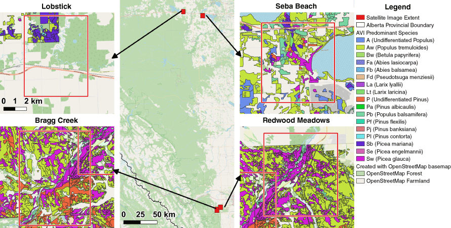
Data are collected within Alberta, Canada, including the boreal, rocky mountain, and foothill natural regions. These regions are relevant to the work performed as all contain coniferous tree stands (Natural Regions Committee 2006) and experience wildfire; in particular, from 1959 to 2021 wildfires in the boreal region accounted for 87.7% of burned area in Alberta (Ahmed 2023). The AVI is consulted to further characterise the areas of study. Due to the large extents of the satellite imagery, numerous tree stands delineated by the AVI are included in each satellite image. As such, the properties listed for each tree satellite image in Table 1 represent an average of the tree stands within the image.
| Satellite image | Natural sub-region | Mean height (m) | Common crown closure (%) | Species present | |||||||
|---|---|---|---|---|---|---|---|---|---|---|---|
| 1 | 2 | 3 | 4 | 5 | 6 | 7 | |||||
| Seba Beach | Boreal–Dry Mixed-wood | 15 | 51–70 | Aw | Sb | Pb | Sw | A | Lt | P | |
| Lobstick | Boreal–Dry Mixed-wood | 9 | 51–70 | Sb | Aw | Pb | Pl | – | – | – | |
| Bragg Creek | Rocky Mountain–Montane | 18 | 51–70 | Sw | Aw | P | Pb | Bw | – | – | |
| Redwood Meadows | Rocky Mountain–Montane | 17 | 51–70 | Aw | Sw | Pb | P | – | – | – | |
Aw, Populus tremuloides; Sb, Picea mariana; Pb, Populus balsamifera; Sw, Picea glauca; A, undifferentiated populus; Lt, Larix laricina; P, undifferentiated pine; Pl, Pinus contorta; Bw, Betula papyrifera.
Satellite imagery is collected via the Pleiades-1 and WorldView-2 platforms, which collect 0.50 m/px panchromatic and 2.0 m/px multispectral products that are pan-sharpened and processed by the vendor into 0.50 m/px RGB imagery covering four communities within these regions in rural Alberta, Canada. The location and coverage of each of these images is in Fig. 1, along with AVI polygons summarising the tree stands.
Extents, locations, and AVI (Forest Stewardship and Trade Branch 2022) of the four satellite images within Alberta.
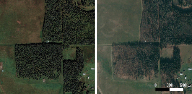
Specifications are set prior to site selection. The images must be free of cloud cover that could obscure areas of interest, the image resolution must be 0.50 m/px, and the angle of global incidence must be less than 30° to ensure trees appear approximately the same across images, and to limit the extent to which taller trees obstruct those behind them. Table 2 summarises the specifications of each satellite image. Two images are acquired for each of the survey areas introduced in Fig. 1: one image in the summer; and another in the winter after tree dormancy but before significant snowfall (Fig. 2). Winter imagery is used for tree classification.
| Survey | Season | Platform | Resolution (m/px) | Capture date | Angle of incidence (°) | Sun elevation (°) | |
|---|---|---|---|---|---|---|---|
| Bragg Creek | Summer | Pleiades-1B | 0.5 | 5 August 2019 | 10.6 | 54.3 | |
| Winter | WorldView-2 | 0.5 | 17 October 2018 | 10.8 | 29.4 | ||
| Redwood Meadows | Summer | Pleiades-1A | 0.5 | 17 July 2018 | 18.9 | 58.6 | |
| Winter | Pleiades-1B | 0.5 | 30 December 2015 | 12.7 | 15.4 | ||
| Seba Beach | Summer | Pleiades-1B | 0.5 | 12 September 2019 | 15.9 | 40 | |
| Winter | Pleiades-1B | 0.5 | 25 October 2015 | 25.0 | 24.3 | ||
| Lobstick | Summer | Pleiades-1B | 0.5 | 15 July 2019 | 9.0 | 56.8 | |
| Winter | Pleiades-1B | 0.5 | 25 October 2015 | 11.5 | 24.2 |
Materials and methods
Individual tree detection
Training data are needed to train a CNN for individual tree detection on summer imagery. Training data are generated by manually annotating 5915 individual trees in 13 square tiles of 150 m side length in three satellite images: (1) Bragg Creek; (2) Seba Beach; and (3) Redwood Meadows (see Supplementary Fig. S1). The Lobstick imagery is held out for testing. Manual annotations generated for each tile are summarised in Table S1. This dataset is used to train a CNN model for individual tree detection from satellite imagery.
To detect individual trees from satellite imagery, a CNN model is trained with the manual annotations. YOLO is a modern CNN architecture that has seen many iterations and improvements, and is tuned for high accuracy and speed (Redmon et al. 2015). At the time of writing, YOLOv8 is considered to be a state-of-the-art object detection framework (Terven and Cordova-Esparza 2023). Training is performed utilising the YOLOv8 API (Jocher et al. 2023).
When training a CNN for a new object detection task, models benefit from ‘pre-initialised weights’, meaning the model has been subject to initial training on premade datasets containing similar objects. These weights can be applied to the model prior to any training done by the researcher. However, detecting trees from satellite imagery is a task quite dissimilar to available premade datasets; trees in satellite imagery are extremely small and image resolution is comparatively low. Thus, to provide the model with weight initialisation, an iterative pretraining scheme is proposed.
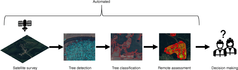
First, the human annotated tiles are used to train a YOLOv8 model with randomly initialised weights. The model is trained for 500 epochs with an initial learning rate of 0.01 and uses the stochastic gradient descent (SGD) optimiser. Additional training parameters are included in Table S2. Due to the small set of human annotations, training is rapid and takes only 30 min. This model is then used to generate predictions across the two satellite images remaining in the training set. These entire satellite images and their corresponding predicted annotations are then tiled, resulting in a large pretraining dataset. A YOLOv8 model is pretrained using these annotations for 200 epochs at an initial learning rate of 0.01. Due to the much larger number of annotations, pretraining takes ~6 h. The pretrained model is then trained using the human annotated dataset for 500 epochs to refine weights; this final model predicts trees in the two satellite images. Fig. 3 depicts this workflow graphically. Model performance is evaluated at each iteration after step 4 and iteration is stopped once negligible performance improvements are observed.
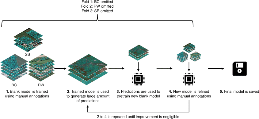
In preparation of the later k-fold assessment procedure, three different models are trained. Each of the models omits one of the surveys (Bragg Creek, BC; Redwood Meadows, RW; or Seba Beach, SB) from the entire training process. Training is performed in an Anaconda Environment on a Windows 10 desktop computer, which is equipped with 256 GB of RAM and an NVIDIA GeForce RTX 4090 GPU. Image augmentations including random flips, modifications to HSV values, and image scaling are applied.
Model performance is assessed by comparing to manual annotations via k-fold cross-validation. In this case, four folds are considered to ensure fairness; in three folds, an entire satellite survey is withheld from the pretraining and training set and used for testing, and one additional ‘arbitrary fold’ is included to demonstrate best possible performance. The arbitrary fold includes all three satellite images, with one training tile from each of the three surveys being randomly removed from training and used for testing.
In a typical object detection assessment, precision, recall and F1-score metrics would be calculated. However, trees in the 0.50 m/px resolution satellite imagery are typically only a few pixels in size, meaning tree bounding boxes are small. The minimum step a bounding box can be placed is 1 px or 0.50 m. As the formula for intersection-over-union (IoU) is calculated as a fraction of area of overlap over area of union, shifting a corner of a bounding box by even a single pixel can result in a low IoU even though the tree is still approximately bounded. The result is that a tree must be boxed with near-perfect accuracy to count as a positive case. This assessment style is unfair to the model, as there may be human error or disagreement between human and machine understanding of where the exact bounds of the tree are interpreted to be. Moreover, in many large-scale applications the exact tree location is less important than a binary measure of ‘was the tree identified or not’. Thus, a metric of stem density is introduced and utilised for model validation. The stem of a tree is defined as the geometric centre of the bounding box that defines it. To calculate density, each tile is gridded and a circle with a 20-m radius is centred on each grid location and the number of stems in each circle is counted. The grid location is then assigned a density value (ntrees/area) in units of trees per m2. To correct for blurring effects at forest boundaries, a second circle is used with a radius of 3 m to set grid locations to 0 if no trees are present. This has the effect of producing sharp boundaries between tree stands and other treeless terrain, such as roads or fields, where density should clearly be considered 0. The manual and machine-predicted stem density grids for each tile are compared. Calculated metrics include R2, root mean squared error, and bias (the mean difference between predicted and true values).
Tree type classification
Tree classification into coniferous/deciduous categories is useful for many exposure assessment and wildfire management processes. Due to the nature of wildfire fuels, detecting coniferous stands is valuable to understanding fire hazard and ember exposure; fires in coniferous areas have the potential to become crown fires with higher fire intensity and rate of spread (Forestry Canada Fire Danger Group 1992).
The use of winter leaf-off and snow free imagery allows for the classification of trees identified by the CNN. Tree boxes generated by the model utilising the georeferenced summer imagery are drawn on the winter imagery. Deciduous tree dormancy and colour-change is leveraged for classification. Trees are categorised as either ‘green-in-winter’ or ‘brown-in-winter’, which are proxies for coniferous and deciduous, respectively. It is useful to detect all trees in summer imagery and then classify with the winter imagery.
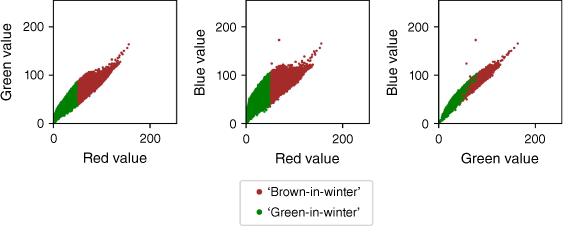
An unsupervised classification method, k-means clustering, is utilised for tree classification. Once tree boxes are drawn on summer imagery, overlaying the boxes to the geographically aligned winter imagery and calculating their colour values is simple. The red (R), green (G), and blue (B) values of pixels within each bounding box are averaged, so that each tree has an average R, G, and B value.
To classify trees, they must first be detected. The tree detection algorithm is applied to the Lobstick imagery, average colour values are calculated for each tree, and the k-means clustering algorithm is applied.
The k-means clustering algorithm is applied to the Lobstick imagery (Fig. 4). An assessment procedure is defined to quantify the accuracy of the k-means algorithm at classifying individual trees. Boxes are compared to manual annotations generated using RPAS survey data (Bennett et al. 2022). RPAS surveys were flown in the same areas as the satellite imagery. A DJI M30T was used with an onboard 1/2″ CMOS camera with an 84° field of view. Flights were conducted at a height of 50 m, and capture images had 80% front overlap and 70% side overlap. Images were then stitched into a 2 cm/px orthomosaic using Agisoft Metashape (Agisoft 2023). At 2 cm/px, RPAS imagery is sufficient to manually classify trees as coniferous or deciduous accurately. To ensure alignment, RPAS orthomosaics were manually adjusted to align with satellite imagery. As every survey contained permanent structures, buildings in RPAS orthomosaics were aligned with their counterparts in satellite imagery. Manual RPAS annotations are taken as the true class of each tree, and the classifications generated by the k-means algorithm are compared. A search is performed for satellite detection boxes and manual RPAS annotation boxes that box the same tree; boxes that overlap are found, and their IoU is calculated and compared to a threshold. If the IoU is greater than the threshold, the boxes are said to be for the same tree and the classes are compared. Performance is assessed at multiple IoU thresholds.
Remote automated exposure mapping
The proposed tree mapping and classification workflow is integrated into existing exposure assessment procedures. Model outputs can be leveraged to generate remote automated exposure maps at a community scale. The method first described in Beverly et al. (2010) and utilised by FireSmart Alberta is used. The community is divided into cells with each cell being graded based on the proportion of nearby landcover occupied by hazardous fuels. Beverly et al. (2010) provides a framework for three assessments: (1) exposure to radiant heat; (2) short-range ember spotting; and (3) long-range ember spotting. In the radiant heat and short-range spotting assessments, the definition of hazard fuels includes grass fuels, which are not the focus of this study. However, exposure to long-range spotting only considers coniferous trees as hazard fuels (Beverly et al. 2010). Further, previous reports have shown that embers are the primary vector for home ignitions (Westhaver 2017).
The steps of a long-range ember exposure assessment described by Beverly et al. (2010) are followed. Beverly et al. (2010) used a combination of site visits, manual imagery interpretation, and consultation with local fire management staff to map hazard fuels. Here, the automated detections and classifications are used as a fuel map. The remaining steps are performed. Structures are manually identified in the satellite imagery, and community bounds are defined as a 100-m buffer around each structure. Finally, a 5-m grid is generated within the community bounds and landcover proportion of hazard fuels surrounding each grid cell is calculated in a 500-m radius.
Hazard fuel landcover proportions are classified into five qualitative ratings (i.e. nil, low, moderate, high, extreme) used by Beverly et al. (2010) (Table S3). Heatmaps are generated by setting the upper bound to the ‘extreme’ proportion in Beverly et al. (2010) and the lower bound to zero. Using these thresholds, remote automated long-range ember exposure maps are created.
Results
Individual tree detection
The model is first pretrained as described and the proposed pretraining process is stopped after no further improvements are observed, taking three generations to stabilise (Fig. 5). This is repeated three times to assess model accuracy, each time leaving one fold out.
Satellite model tree detection performance at each generation for each of the folds in Seba Beach (SB), Redwood Meadows (RW), and Bragg Creek (BC).
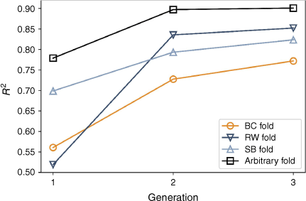
Generation 2 was the first generation to receive pretraining, and a significant increase in performance is observed. The third iteration results in less benefit and iteration is stopped. The difference in performance between the folds that withheld entire surveys and arbitrary fold quantifies the expected performance reduction due to the variation in satellite imagery; the BC, RW, and SB folds are a fairer assessment procedure than testing on tiles from the same satellite survey used in training (arbitrary fold). Average R2 values reach 0.82 in the third generation (Table 3) and average RMSE values are 89 boxes/ha. Average R2 values in the first generation only reached an average of 0.59, showing the generational training process increased performance by 0.23. A detailed analysis of the results from the final generation is provided where generated densities are compared to manual annotation densities (Fig. 6).
| Generation 3 | R2 | RMSE (boxes/ha) | Bias (boxes/ha) | |
|---|---|---|---|---|
| BC fold (five tiles) | 0.77 | 54 | −26 | |
| RW fold (five tiles) | 0.85 | 129 | 108 | |
| SB fold (three tiles) | 0.82 | 85 | −48 | |
| Average | 0.82 | 89 |
Detection density crossplots for final generation for each cell in each tile in each fold. Points are coloured based on the density of points for clarity, yellow being more dense. All axes are equal.
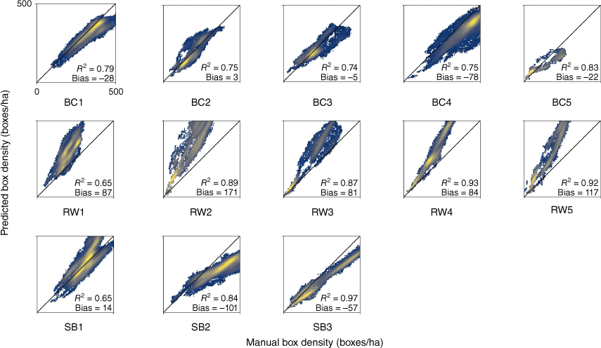
Bias is shown in the results (Fig. 6). Bragg Creek is generally negatively biased, while Redwood Meadows is positively biased. Tree detection densities in the Redwood Meadows survey are consistently overpredicted (Fig. 6); this survey had the highest angle of incidence (19°) of all surveys in this study, causing the algorithm to double-box trees by placing one small square box at the bottom of the tree and another small square box at the top, while manual annotations correctly box the entire tree using a vertical rectangle. In the future, additional surveys should be collected to expand the training set and allowing for diverse angles of incidence in every training set. This addresses the problem of dataset shift; many factors can affect the appearance of satellite imagery between surveys including lighting, angle of incidence, season, and atmospheric conditions. Overall, performing a three-fold assessment wherein test surveys are not included in any training steps provides an assessment of the robustness of the model to dataset shift.
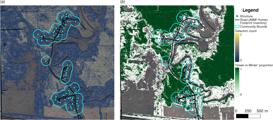
Results can be assessed visually. The tree detection and classification workflows are applied to the Lobstick imagery, which was not used for model training. The workflow quickly and automatically outputs 1,373,224 tree detections in the 3050-ha area, and the classification procedure separates these into 966,932 ‘green-in-winter’ and 406,292 ‘brown-in-winter’ detections. Binned detection density maps (counting each tree detection box as a tree stem instance) can be generated to visualise ‘green-in-winter’ tree detections across large scales (Fig. 7b).
(a) Satellite image, (b) binned density map of satellite detections for ‘green-in-winter’ trees, and (c) 100-m detection density assessment of a community in rural Alberta.
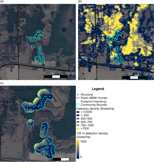
The relative density of hazardous tree detections surrounding a community can also be assessed. Fig. 7c grids the community into 5-m cells and uses a 100-m radius around each cell to calculate local detection density (boxes/ha). Though the model is unable to distinguish between fuel types, considerations can be made regarding the classification of trees into ‘green-in-winter’ or ‘brown-in-winter’ categories, and calculated densities are shown to correlate with manual annotations. It is noted that densities calculated here are expected to underestimate actual tree densities, as satellite imagery is limited to the overstorey, and the resolution of 0.50 m/px limits detections to only large trees.
Tree type classification
The assessment procedure previously outlined is applied to the detections generated for the Lobstick imagery (Table 4) comparing to the reliable RPAS-based classification. The average F1-score for classification is 0.85 for coniferous and 0.82 for deciduous trees. As expected, the number of matches drops significantly as the IoU threshold increases; this is due to the issues with IoU calculation on low-resolution imagery mentioned earlier, imperfect alignment between RPAS and satellite imagery, and time difference between surveys. Visual assessments are also generated (Fig. 8). Tree detection and classification is also qualitatively compared to existing Canadian Forest Fire Behaviour Prediction (FBP) System fuel type maps for the area. These maps are generated by first utilising a kNN procedure to map forest attributes across the nation at 50-m resolution, and then using a set of rules to convert the attribute map into FBP fuel types (Hirsch 1996; Beaudoin et al. 2014; Natural Resources Canada 2019) (Fig. 8).
| IoU | Total matches found | Conifer precision | Conifer recall | Deciduous precision | Deciduous recall | Conifer F1 | Deciduous F1 | |
|---|---|---|---|---|---|---|---|---|
| 0.1 | 7564 | 0.88 | 0.90 | 0.84 | 0.80 | 0.89 | 0.82 | |
| 0.2 | 3281 | 0.84 | 0.88 | 0.84 | 0.81 | 0.86 | 0.82 | |
| 0.3 | 1515 | 0.81 | 0.87 | 0.85 | 0.79 | 0.84 | 0.82 | |
| 0.4 | 679 | 0.79 | 0.87 | 0.86 | 0.78 | 0.83 | 0.82 | |
| 0.5 | 290 | 0.77 | 0.86 | 0.85 | 0.75 | 0.81 | 0.79 | |
| Average | 0.82 | 0.88 | 0.85 | 0.78 | 0.85 | 0.82 | ||
(a) Summer and (b) winter satellite imagery in rural Alberta. Classification results are shown in (c) and compared to the local fuel map (Beaudoin et al. 2014) in (d).
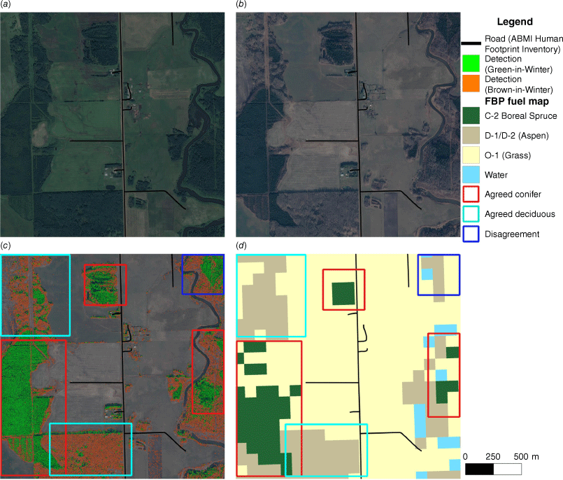
Both maps (Fig. 8) identify hazard fuels in the west, north, and east portions of the image, highlighted with a red box. Trees in the south and northwest portions can be classified as ‘brown-in-winter’, shown using a cyan box. There is some disagreement in the northeast (blue box); closer examination of the winter satellite image suggests the fuel map may be in error as the area is classified as fuel type O-1 (grass) in an area where trees clearly exist.
Remote automated exposure mapping
Tree detection and classification is performed with the proposed workflow for a community in rural Alberta (Fig. 9a). Structure locations are manually interpreted from the imagery, and a 100-m ‘community buffer’ is drawn around each to define the community bounds.
(a) Satellite image, (b) satellite image with classified tree detections, (c) binned long-range ember exposure assessment, and (d) heatmap of long-range ember exposure for community in rural Alberta.
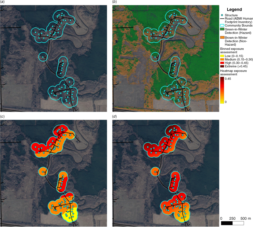
Using ‘green-in-winter’ tree detections as a hazard fuel map, hazard land cover proportions surrounding each cell are calculated as in Beverly et al. (2010). Fig. 9c includes bins based on the Beverly et al. (2010) thresholds (Table S3) and a proportional heatmap (Fig. 9d) of nearby hazard fuel landcover.
Portions of the community along the WUI that closely abut ‘green-in-winter’ forested areas have high exposure, while those further to the interior and south have medium and low exposure ratings (Fig. 9). All four areas are deemed to have some exposure to long-range spotting, but the analysis need not be limited to specific community bounds; exposure can be mapped across the entire area of interest (Fig. S2).
It is important to note that these figures do not represent full community assessments, rather they are intended to supplement existing practices (Beverly et al. 2010, 2018) and are thus dubbed a ‘mock assessment’. The model is only able to detect overstorey without consideration for understorey and surface fuels. These aspects are critical to community assessment; the proposed workflow is suggested as a source of supplemental information, rather than as a stand-alone hazard assessment tool.
Discussion
Individual tree detection
Tree prediction accuracy is assessed at a large scale in the satellite imagery workflow by comparison with manual annotations; densities are shown to correlate well between predicted and manually identified trees, reaching an average R2 of 0.82 (Table 3). Results at Redwood Meadows show strong positive bias: due to the angle of incidence, trees are often double boxed by the algorithm, resulting in overestimated densities. It is noted that this would not affect a landcover-based assessment such as the exposure assessment procedure as only area occupied by hazard fuels is measured rather than tree stem density. The algorithm does not perfectly detect every individual tree and should not be used in situations and scales where every tree is important, such as structure level exposure or triage assessments (Partners in Protection 2003; Alberta Wildfire 2020). This result remains compelling when compared to current research. Yao et al. (2021) utilised a similar assessment method (comparing measurements of manually identified and automatically detected tree densities) and achieved an R2 score of 0.933. The methodology and goals of the study differed; individual trees in Yao et al. (2021) are not detected using a bounding box. Instead, Yao et al. (2021) output points on tree stems, and thus trees are not sized nor classified. This method was beneficial, as more training data were generated due to the simplified detection process (stem point instead of sized and located bounding box). The results of the arbitrary fold in Fig. 5 suggest that additional training data may allow this study to achieve similar results to Yao et al. (2021), as the developed CNN would be less sensitive to domain shifts in training data. Results are also compared to the work of Gomes et al. (2018), who use Marked Point Processes to detect and delineate tree crowns in WorldView-2 imagery, and achieve detection accuracies from 0.81 to 0.95, with delineation accuracy lower at 0.63. Gomes et al. (2018) also encounter the issue of multiple detections placed on single large trees. However, the workflow presented relies on tree shadows for crown detection, and thus is only applied to ‘trees outside of forests’ and not in dense stands. A number of studies exist that count plantation trees from satellite imagery, but trees in these studies are typically from a single species, evenly spaced, and have little crown overlap, especially when compared to the conditions of the present study involving dense natural tree stands (Mubin et al. 2019; Vermote et al. 2020; Abozeid et al. 2022). Overall, this study presents tree detection results comparable to other state-of-the-art results.
In the context of hazard management, errors of omission are more significant as they could lead to underestimating hazard. Because sensitivity is not prioritised, locations identified as hazardous within a community should be verified by other means, such as a RPAS survey or in situ assessment. Further, while the tree detection model is assessed by comparing detection densities to manual annotation densities, further validation should assess the correlation between detection density and forest density measured in situ. Validating the model compared to field measurements and searching for a relationship between field densities and detection densities could extend the application cases of the model.
Tree detections in all overhead imagery are limited to detection of overstorey trees; trees in the understorey are occluded and cannot be detected. As the model is trained using human annotations, trees must also be of sufficient size so as to be discernable in the 0.50 m/px imagery. Finally, in dense stands where tree crowns overlap, human and machine annotations alike identify the large, prominent overstorey. Wildfire fuels other than overstorey trees (such as duff, grass, small trees, and ground litter) are also not assessed by this method, although other studies classify grasslands (Badreldin et al. 2021).
Stand attributes are omitted in this workflow. The hazard fuels used in the above assessment are individual ‘green-in-winter’ tree detections; these detections are not aggregated into stand-level patches. As such, mixedwood stands are not classified as they were in Beverly et al. (2010). However, a benefit of individual tree detection is the possibility for aggregation into fuel maps at any resolution. In Fig. 10, a 5-m grid is considered and tree count is calculated within each cell. The proportion of ‘green-in-winter’ trees within each cell is also calculated. It would be valuable to investigate and validate the use of calculated metrics to aggregate detections into stand-level attributes. Future work would also identify opportunities for integration into CFFDRS-2025, which utilises input maps of stem density, tree species, proportion coniferous/deciduous, and canopy closure. However, caution should be used as significant overpredictions were seen in the Redwood Meadows study area, likely due to the high angle of incidence. Additional training data should be generated to increase model robustness.
Tree type classification
Tree classification from satellite imagery also proves accurate when compared to manual annotations from RPAS imagery. While the satellite classification algorithm classifies trees based on colour and bins them into ‘green-in-winter’ and ‘brown-in-winter’ categories, the predictions were compared to trees in RPAS imagery that could be definitively stated to be coniferous or deciduous; the predictions made by the satellite algorithm were seen to be correct above 80% of the time. The resulting accuracy is encouraging, as when considered with the detection score it is seen that trees can be detected and classified accurately from satellite imagery. However, it should be noted that ‘green-in-winter’ and ‘brown-in-winter’ remain a proxy for coniferous and deciduous trees, respectively; coniferous trees such as larch that go dormant in the winter, or areas where coniferous trees have been subject to attack by pest or disease may cause classification errors, resulting in under-estimated hazard.
The classification method is consistent with other literature surrounding tree classification from satellite imagery. Many studies exist that leverage leaf-off imagery to classify trees. Hoff et al. (2018) use 0.39 m/px leaf-off satellite imagery to map the encroachment of eastern red cedar stands into regions typically dominated by oak species. Authors leverage the colour difference in leaf-off imagery and find the approach effective for identifying and estimating canopy area and above ground biomass for eastern red cedar, noting the relevance to wildfire. However, properties are still calculated at the stand level, and individual trees are not identified nor classified. Sapkota and Liang (2018) use both leaf-on 1 m/px aerial imagery and leaf-off 0.46 m/px multispectral WorldView-2 satellite imagery in Arkansas to locate non-forest areas and to classify trees as ‘canopied’ or ‘leafless’. Authors test both a decision tree and nearest neighbour approach for classification, reaching an accuracy of 89%; it is noted that this work required the generation of training samples to fit the chosen models. Together, it is clear that the utilisation of leaf-off imagery is commonly utilised for tree classification and motivates the approach taken by the present study; which in comparison does not require training data, does not require non-forest areas to first be removed using aerial imagery, and outputs tree classifications at the individual-tree scale.
In the future, utilising additional spectral bands should be investigated to increase classification accuracy and reliability and potentially eliminate the need for proxy classes. Overall, detecting and classifying trees at this resolution can enable extremely high-resolution mapping across large spatial areas.
Remote automated exposure mapping
The workflow proposed offers a remote automated method of assessing wildfire exposure at a large scale (Fig. 11). When the maps are compared to existing fuel maps, the difference in resolution is apparent; Fig. 8 demonstrates the resolution difference between the maps generated by the workflow outlined in this study and a 100-m Alberta Fuel Map. Differences between the AVI and this procedure are also noted; while the AVI estimates additional forestry parameters such as mean height, crown closure, and specific species, the AVI workflow consists of the manual interpretation of imagery dating as far back as 1988. Further, coverage is occasionally lacking (Fig. 1) as the community assessed in this paper lacked comprehensive AVI stand characterisations. The developed workflow in this paper is automated and could be applied to any domain where satellite imagery matching the specifications (0.50 m/px, summer and winter, <30° off-nadir) can be acquired and the appearance of trees in said imagery is similar to the domain of the study (boreal, rocky mountain, and foothill natural regions in Alberta). While Fig. 9 demonstrates the applicability of this workflow to a community, Fig. S2 demonstrates how this method could be broadly applied to an entire region, subject to satellite image availability. FireSmart initiatives to reduce WUI fire risk could potentially be facilitated with this method, simplifying hazard detection for the application of mitigation techniques and subsequent reassessment. Current guidelines recommend communities adopt a vegetation management regime composed of three activities: (1) fuel removal; (2) fuel reduction; and (3) species conversion (Government of Alberta 2013). Fuel removal involves the removal of flammable tree species at key points around the community or structure of interest in order to create fire breaks or defensible spaces, lowering the propensity of wildfire to rapidly spread to houses or infrastructure. Species conversion reduces flammability within communities by substituting flammable trees with less flammable varieties. Tree detections from satellite imagery are available on a large spatial scale and can be used to supplement the planning of mitigation activities.
The proposed tree classification workflow and application to detections in the context of exposure assessment is limited as it defines only ‘green-in-winter’ trees as hazard fuels. This proxy for coniferous/deciduous means that tree species such as larch, or conifers experiencing disease or pests, would be classified as a non-hazard, which would artificially lower the calculated exposure rating.
The availability and recency of satellite imagery should be considered; imagery is not always available at the resolution and specifications required. Despite having return periods as short as 1 day, this varies significantly depending on the location of the area of interest. Further, conditions may be unfavourable for satellite imagery capture on the day the satellite passes the area of interest. In Canada, the boreal forest may be snow covered or dormant for much of the year, leaving only a few months where ‘summer’ and ‘snow free leaf-off’ imagery can be collected. The collection of this imagery may be further impeded by clouds and other atmospheric conditions. Depending on the orbit of the satellite capturing the area, the angle off-nadir may also be too significant for the algorithm to be reliably applied. These limitations can result in a time-lag between the present day and the date when suitable satellite imagery can be collected. Imagery used in this study ranges from 2015 to 2021. The nature and resolution of satellite imagery also limits the trees that can be detected. Optical satellite imagery cannot penetrate the top canopy and 0.50 m/px resolution means small trees cannot be resolved; thus, only large overstorey trees are detected. It is worth noting that the exposure maps generated treated ‘brown-in-winter’ stands as non-hazardous fuels. As mentioned in Beverly et al. (2021), stands presenting with deciduous overstories but developed spruce understoreys can be capable of generating long-range embers, increasing the actual exposure of the community.
This section explores a wildfire exposure assessment, rather than a full threat or risk assessment. The R11 Forest Management Plan, a document that outlines forest management activities for the R11 Forest Management Unit in Alberta Canada, provides an example of a wildfire threat assessment (Alberta Sustainable Resource Development 2007). The threat assessment contains four components – fire behaviour potential, fire occurrence risk, values at risk, and suppression capability. While the proposed method identifies and classifies trees, its outputs are not sufficient to inform fire behaviour potential mapping, which considers additional fuel attributes, topography and climate.
While identifying exposure levels can be valuable for planning mitigation activities and response efforts, these analyses do not assess risk, which requires the joint consideration of ignition probability, ability for resources to respond to an incident, values-at-risk (VAR), and a full characterisation of hazards present (Alberta Sustainable Resource Development 2007).
Conclusion
The three key factors in wildfire behaviour are fuel, weather, and topography. Of these three components, only fuels can be managed proactively in advance of a fire. A remote automated tree detection and classification workflow is proposed to detect and classify individual trees and was validated by comparison to manual photo interpretation. In the future, field validation to stem density may be required to assess the workflows accuracy to ground conditions.
Mitigation planning and suppression efforts can benefit from reliable, recent, and high-resolution fuel attribute data. Remote sensing combined with machine learning is shown to reproduce manual photo interpretation, identify large overstorey trees, and classify them into proxy categories for coniferous/deciduous, creating a rough fuel attribute map at a high spatial resolution.
The ability to delineate trees that remain ‘green-in-winter’ shows potential for aiding in mitigation planning. Direct application of model outputs to community level exposure assessments provides value but does not replace current best practice. Maps presented demonstrate the use of classified tree detections identified from satellite imagery in a mock exposure assessment of a community in rural Alberta. Overall, the study presents a framework for a remote automated photo interpretation workflow that could provide extremely high-resolution maps (individual tree scale) of coniferous and deciduous trees, across large spatial extents, and for any time in which appropriate summer and winter satellite imagery is available.
References
Abozeid A, Alanazi R, Elhadad A, Taloba AI, Abd El-Aziz RM (2022) A large-scale dataset and deep learning model for detecting and counting olive trees in satellite imagery. Computational Intelligence and Neuroscience 2022, 1549842.
| Crossref | Google Scholar |
Agisoft (2023) Agisoft Metashape Professional. Available at https://www.agisoft.com/features/professional-edition/
Ahmed MR, Hassan QK (2023) Occurrence, area burned, and seasonality trends of forest fires in the Natural Subregions of Alberta over 1959–2021. Fire 6(3), 96.
| Crossref | Google Scholar |
Airbus Defense and Space Intelligence (2012) Pléiades. Airbus. (Taufkirchen: Germany). Available at https://intelligence.airbus.com/imagery/our-optical-and-radar-satellite-imagery/pleiades/
Alberta Wildfire (2020) ‘Wildland Urban Interface Triage Assessment Form.’ (Edmonton, AB, Canada) Available at https://open.alberta.ca/dataset/58d44774-be40-411b-96a9-0f4b175c902a/resource/53f6a266-739a-461e-b61a-3acf673f7fc8/download/ma-alberta-wildland-interface-fire-structure-protection-guidelines-2020.pdf
Badreldin N, Prieto B, Fisher R (2021) Mapping grasslands in mixed grassland ecoregion of Saskatchewan using big remote sensing data and machine learning. Remote Sensing 13, 4972.
| Crossref | Google Scholar |
Beaudoin A, Bernier PY, Guindon L, Villemaire P, Guo XJ, Stinson G, Bergeron T, Magnussen S, Hall RJ (2014) Mapping attributes of Canada’s forests at moderate resolution through kNN and MODIS imagery. Canadian Journal of Forest Research 44, 521-532.
| Crossref | Google Scholar |
Bennett L, Wilson B, Selland S, Qian L, Wood M, Zhao H, Boisvert J (2022) Image to attribute model for trees (ITAM-T): individual tree detection and classification in Alberta boreal forest for wildland fire fuel characterization. International Journal of Remote Sensing 43, 1848-1880.
| Crossref | Google Scholar |
Beverly JL, Bothwell P, Conner JCR, Herd EPK (2010) Assessing the exposure of the built environment to potential ignition sources generated from vegetative fuel. International Journal of Wildland Fire 19, 299-313.
| Crossref | Google Scholar |
Beverly JL, McLoughlin N, Chapman E (2021) A simple metric of landscape fire exposure. Landscape Ecology 36, 785-801.
| Crossref | Google Scholar |
Brandt JP, Flannigan MD, Maynard DG, Thompson ID, Volney WJA (2013) An introduction to Canada’s boreal zone: ecosystem processes, health, sustainability, and environmental issues. Environmental Reviews 21, 207-226.
| Crossref | Google Scholar |
Canadian Forest Service Fire Danger Group (2021) An overview of the next generation of the Canadian Forest Fire Danger Rating System. Information Report GLC-X-26. Available at https://ostrnrcan-dostrncan.canada.ca/handle/1845/245411
Deur M, Gašparović M, Balenović I (2021) An evaluation of pixel- and object-based tree species classification in mixed deciduous forests using pansharpened very high spatial resolution satellite imagery. Remote Sensing 13, 1868.
| Crossref | Google Scholar |
DigitalGlobe (2009) WorldView-2. Available at https://www.spaceimagingme.com/downloads/sensors/datasheets/WorldView2-DS-WV2-Web.pdf
Freudenberg M, Magdon P, Nölke N (2022) Individual tree crown delineation in high-resolution remote sensing images based on U-Net. Neural Computing and Applications 34, 22197-22207.
| Crossref | Google Scholar |
Gomes MF, Maillard P, Deng H (2018) Individual tree crown detection in sub-meter satellite imagery using Marked Point Processes and a geometrical-optical model. Remote Sensing of Environment 211, 184-195.
| Crossref | Google Scholar |
Government of Alberta (2013) ‘FireSmart Guidebook for Community Protection: A Guidebook for Wildland/Urban Interface Communities.’ (Edmonton, AB). Available at https://wildfire.alberta.ca/firesmart/documents/FireSmart-GuideCommunityProtection-Nov2013.pdf
Hoff DL, Will RE, Zou CB, Weir JR, Gregory MS, Lillie ND (2018) Estimating increased fuel loading within the Cross Timbers forest matrix of Oklahoma, USA due to an encroaching conifer, Juniperus virginiana, using leaf-off satellite imagery. Forest Ecology and Management 409, 215-224.
| Crossref | Google Scholar |
Jocher G, Chaurasia A, Qiu J (2023) YOLO by Ultralytics. Available at https://github.com/ultralytics/ultralytics
Johnston LM, Flannigan MD (2018) Mapping Canadian wildland fire interface areas. International Journal of Wildland Fire 27, 1-14.
| Crossref | Google Scholar |
Kattenborn T, Leitloff J, Schiefer F, Hinz S (2021) Review on Convolutional Neural Networks (CNN) in vegetation remote sensing. ISPRS Journal of Photogrammetry and Remote Sensing 173, 24-49.
| Crossref | Google Scholar |
Linn RR, Goodrick SL, Brambilla S, Brown MJ, Middleton RS, O’Brien JJ, Hiers JK (2020) QUIC-fire: a fast-running simulation tool for prescribed fire planning. Environmental Modelling & Software 125, 104616.
| Crossref | Google Scholar |
Mubin NA, Nadarajoo E, Shafri HZM, Hamedianfar A (2019) Young and mature oil palm tree detection and counting using convolutional neural network deep learning method. International Journal of Remote Sensing 40, 7500-7515.
| Crossref | Google Scholar |
Natesan S, Armenakis C, Vepakomma U (2020) Individual tree species identification using Dense Convolutional Network (DenseNet) on multitemporal RGB images from UAV. Journal of Unmanned Vehicle Systems 8, 310-333.
| Crossref | Google Scholar |
Natural Resources Canada (2019) ‘Canadian Forest FBP Fuel Types (CanFG).’ (Canadian Forestry Service, Northern Forestry Centre: Edmonton, AB) Available at https://cwfis.cfs.nrcan.gc.ca/downloads/fuels/development/
Redmon J, Divvala S, Girshick R, Farhadi A (2015) You Only Look Once: Unified, Real-Time Object Detection. 10.48550/arXiv.1506.02640
Sapkota BB, Liang L (2018) A multistep approach to classify full canopy and leafless trees in bottomland hardwoods using very high-resolution imagery. Journal of Sustainable Forestry 37, 339-356.
| Crossref | Google Scholar |
Stocks BJ, Lynham TJ, Lawson BD, Alexander ME, Wagner CE Van, McAlpine RS, Dubé DE (1989) The Canadian Forest Fire Danger Rating System: an overview. The Forestry Chronicle 65, 450-457.
| Crossref | Google Scholar |
Surový P, Kuželka K (2019) Acquisition of forest attributes for decision support at the forest enterprise level using remote-sensing techniques—A review. Forests 10, 273.
| Crossref | Google Scholar |
Terven J, Cordova-Esparza D (2023) A Comprehensive Review of YOLO: From YOLOv1 and Beyond. Available at http://arxiv.org/abs/2304.00501.
Van Wagner CE (1977) Conditions for the start and spread of crown fire. Canadian Journal of Forest Research 7, 23-34.
| Crossref | Google Scholar |
Varin M, Chalghaf B, Joanisse G (2020) Object-based approach using very high spatial resolution 16-Band WorldView-3 and LiDAR data for tree species classification in a broadleaf forest in Quebec, Canada. Remote Sensing 12, 3092.
| Crossref | Google Scholar |
Vermote EF, Skakun S, Becker-Reshef I, Saito K (2020) Remote sensing of coconut trees in Tonga using very high spatial resolution WorldView-3 data. Remote Sensing 12, 3113.
| Crossref | Google Scholar |
Yao L, Liu T, Qin J, Lu N, Zhou C (2021) Tree counting with high spatial-resolution satellite imagery based on deep neural networks. Ecological Indicators 125, 107591.
| Crossref | Google Scholar |