

Generating fuel consumption maps on prescribed fire experiments from airborne laser scanning
T. Ryan McCarley A , Andrew T. Hudak B * , Benjamin C. Bright B , James Cronan C , Paige Eagle D , Roger D. Ottmar C and Adam C. Watts C
A
B
C
D
Abstract
Characterisation of fuel consumption provides critical insights into fire behaviour, effects, and emissions. Stand-replacing prescribed fire experiments in central Utah offered an opportunity to generate consumption estimates in coordination with other research efforts.
We sought to generate fuel consumption maps using pre- and post-fire airborne laser scanning (ALS) and ground measurements and to test the spatial transferability of the ALS-derived fuel models.
Using random forest (RF), we empirically modelled fuel load and estimated consumption from pre- and post-fire differences. We used cross-validation to assess RF model performance and test spatial transferability.
Consumption estimates for overstory fuels were more precise and accurate than for subcanopy fuels. Transferring RF models to provide consumption estimates in areas without ground training data resulted in loss of precision and accuracy.
Fuel consumption maps were produced and are available for researchers who collected coincident fire behaviour, effects, and emissions data. The precision and accuracy of these data vary by fuel type. Transferability of the models to novel areas depends on the user’s tolerance for error.
This study fills a critical need in the broader set of research efforts linking fire behaviour, effects, and emissions.
Keywords: airborne laser scanning (ALS), emission source, FASMEE, fire, Fishlake National Forest, fuel beds, fuel consumption, Monroe Mountain, prescribed fire, stand-replacing.
Introduction
Characterisation of the structure and arrangement of combustible biomass on the landscape provides important insight into fire behaviour, effects, and emissions (Ottmar 2014; Van Der Werf et al. 2017; Prichard et al. 2019). These materials, commonly referred to as fuel, are often subdivided into categories such as fuel beds, which represent materials with specific physical characteristics leading to differing fire behaviour (Ottmar et al. 2007; Riccardi et al. 2007; Keane et al. 2013). The three-dimensional nature of fuels, collectively and as individual fuel beds, suggests the importance of spatially explicit methods of quantification (Hudak et al. 2020; Taneja et al. 2021). Airborne laser scanning (ALS) data fit this need, being able to capture both the vertical and horizontal distribution of fuel across a landscape (Chuvieco et al. 2020).
Empirical models using ALS data trained with in-situ measurements of fuel load (i.e. the mass of fuel per area [Mg ha−1]) have been shown effective at quantifying canopy fuel load (e.g. Andersen et al. 2005; Skowronski et al. 2011; Mauro et al. 2021). These types of models also have demonstrated utility for estimating loading of subcanopy surface fuels (e.g. Price and Gordon 2016; Stefanidou et al. 2020; Alonso-Rego et al. 2021; Mauro et al. 2021), despite lower accuracies due to canopy occlusion and the inherently high heterogeneity of fuels (Bright et al. 2022). Furthermore, analysis of multitemporal ALS (i.e. the use of two or more ALS datasets across time) has demonstrated effectiveness for estimating fuel consumption in the canopy and subcanopy (McCarley et al. 2020, 2022; Bright et al. 2022).
Due to the interrelated nature of fuel consumption, fire behaviour, heat release, plume dynamics, and smoke chemistry, there is a need for large scale interdisciplinary research endeavours to understand complex relationships, employ new technology, and make new discoveries (Peterson and Hardy 2016; Prichard et al. 2019). To meet this need, coordinated research efforts were conducted as part of the Fire and Smoke Model Evaluation Experiment (FASMEE) on five stand-replacing prescribed fires on the Fishlake National Forest in central Utah, USA (Prichard et al. 2019; Ottmar et al. 2021). Pre- and post-fire ALS data were acquired along with pre- and post-fire fuel load measurements on the ground, thereby providing the measurement data needed to generate spatially explicit estimates of fuel consumption. These can be used to understand relationships between fuel consumption and measurements of fire behaviour, heat release, plume dynamics, and smoke composition related to FASMEE. Users of these data may also be interested in the spatial transferability of the models to other areas of similar forest type where ALS data are available, but associated plot data are not. Therefore, in this study, we (1) estimate fuel consumption at five prescribed fires and (2) test the spatial transferability of the ALS-derived fuel models to estimate fuel consumption by separating the plot data into training and validation sets.
Materials and methods
Study area
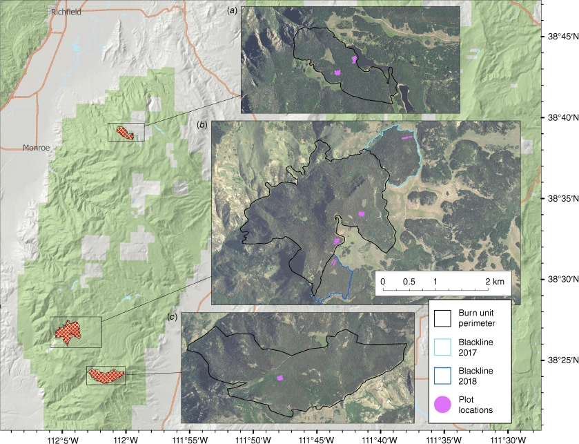
Stand-replacement fires are operationally prescribed on subalpine forests in the Fishlake National Forest, with a primary objective of removing older beetle-killed or encroaching younger conifers and reestablishing quaking aspen (Populus tremuloides). Five prescribed fires in 2017–2020 provided FASMEE researchers with opportunities to collect measurements on fuels, fire behaviour, heat release, plume processes, smoke emissions, and fire effects on vegetation and soil (Ottmar et al. 2021). The main FASMEE burn units (Fig. 1) were the Manning Creek Unit (MCU) burned on 20 June 2019, the Langdon Mountain Unit (LMU) burned on 7 November 2019, and the Annabella Reservoir Unit (ARU) burned on 5 November 2020. Two additional prescribed burns were conducted adjacent and prior to (October 2017 and 21 November 2018) the MCU burn to act as firebreaks, referred to hereafter as Blackline (BL) units (i.e. BL2017 and BL2018; Fig. 1). Fuel moisture on the day of burning was much higher at ARU than all other units due to snow (~35% for 1- and 10-h fuels). LMU had the lowest fuel moisture (~10% for 1- and 10-h fuels; MCU: ~15%). See DRIScience (2020) for an overview of the FASMEE project and video footage from within the MCU as an example of fire behaviour.
Overview of the three burn units on Monroe Mountain in the Fishlake National Forest south of Richfield, UT: (a) Annabella Reservoir (ARU), (b) Manning Creek (MCU) and adjacent blackline units (burned in 2017 on the northeast edge of the MCU and in 2018 on the southern edge of the MCU), (c) Langdon Mountain (LMU). Plots (n = 61) were clustered into seven sampling areas.
Elevations ranged from 2449 m at MCU to 3212 m at ARU, with a mean elevation of 2908 m across all units. The burn units were mostly forested with quaking aspen, sub-alpine fir (Abies lasiocarpa), and Engelmann spruce (Picea engelmannii), with open areas of sagebrush (Artemisia sp.) acting as natural firebreaks on the unit edges. None of the burn units had experienced fire for over 150 years (Linda Chappell, personal communication).
Field data
Between 2016 and 2021, 61 plots were sampled twice (i.e. pre and post-fire) in MCU (n = 20), LMU (n = 10), ARU (n = 20), BL2017 (n = 6), and BL2018 (n = 5) by the Fire and Environmental Research Applications Team of the USDA Forest Service (Fig. 1). Plots were divided between seven sampling areas (5–20 plots per area) and systematically arranged on a grid within each sampling area. These sampling areas were distributed across the three main burn units and two blackline units to represent the range of forest types (Ottmar et al. 2021). Each plot was defined by a centre point geolocated using a Javad Triumph-2 differential GPS (Javad GNSS, Inc., San Jose, CA). To estimate litter and duff fuel loads, we measured litter and duff depths at eight points per plot, computed an average depth for each material, then multiplied it by published material-specific fuel bed density values (Prichard et al. 2017). Coarse (100- and 1000-h) down woody debris (DWD) was calculated following Brown et al. (1982) using measurements along three 10 m transects extending radially from plot centre, based on a single random azimuth then spaced equally 120° apart. Each plot had two nested 1 m2 clip plots placed 5 m from plot centre, oriented at 0° (north) and 180° (south). The northern clip plot was used to collect pre-fire fuels and the southern for post-fire fuels. Herbaceous fuels, shrubs, and seedlings were clipped (destructively sampled) then oven-dried and weighed to obtain fuel loading, while fine DWD (1- and 10-h) were collected (destructively sampled) within one quadrant (0.25 m2) of the clip plot. For canopy fuel, we recorded species, status (live/dead), and measured the DBH of all trees (>12 cm DBH) within an 8 m radius from plot centre. Additionally, total height, height to live crown, and canopy base height were measured for a subset of live trees. Saplings (≤12 cm DBH and >1.37 m tall) were tallied within a 5.6 m radius and an average sapling DBH was used. We calculated fuel load for trees (i.e. boles, snags, and crown material), saplings, and available canopy fuel (ACF) (i.e. foliage plus 50% of fine branches) using the Fire and Fuels Extension of the Forest Vegetation Simulator (Reinhardt and Crookston 2003). Additional details on field data collected and plot design can be found in Ottmar et al. (2021).
ALS data
Pre-fire ALS data were collected by Digital Mapping Inc. using an Optech ALTM 167 GEMINI sensor between 27 August and 11 September 2016 at ≥8 pulses/m2 and with 60% overlap. Post-fire ALS data were collected by Technical Applications and Consulting, LLC using an Optech Galaxy T500 sensor. Post-fire ALS data for MCU, LMU, BL2017, and BL2018 were collected on 30 September 2020 at ≥8 pulses/m2 and with 80% overlap, while data for ARU were collected on 15 June 2021 at ≥7 pulses/m2 and with 100% overlap. Using LAStools (Isenburg 2013), we normalised the height of the ALS point clouds, then calculated statistical metrics (e.g. height percentiles, canopy cover, point density in height strata; Supplementary Table S1) within 8 m circles at each plot (i.e. the area within which trees were tallied) from both the pre- and post-fire ALS acquisitions. The same statistical metrics were calculated for 10 m raster grids across each ALS acquisition.
Data analysis
We trained RF models to predict fuel loading of canopy (trees and saplings), shrub/seedling, herbaceous, DWD, litter, duff, total fuel, subcanopy fuel (shrub/seedling, herbaceous, DWD, litter, and duff), and ACF using the combined set of pre- and post-fire field data as the independent observations and the corresponding pre- and post-fire ALS statistical metrics within the 8 m circles of each plot as the predictor variables. We used an iterative variable selection process to reduce the number of final predictor variables (McCarley et al. 2020, 2022; Supplementary Table S1). To estimate fuel consumption across the burn units, we predicted pre- and post-fire fuel load using the RF models to 10 m rasters, then differenced them.
To assess the quality of the RF fuel loading models, we evaluated variance explained (i.e. pseudo-R2) reported in the RF outputs. We validated consumption estimates in three ways: (1) comparing estimated fuel consumption to observed fuel consumption at all the plots; (2) performing 3-fold cross-validation, where data were selected for each fold at random, irrespective of burn unit; and (3) performing a geographic 3-fold cross-validation, where the training and validation plot subsets were separated between the burn units of unequal sample size (Fig. 1). Fit statistics of root mean squared error (RMSE) and %RMSE (i.e. RMSE divided by the mean of observed values) and mean bias estimate (MBE) (i.e. the mean of predicted minus observed values) and %MBE (i.e. MBE divided by the mean of observed values) were used to assess the models and make comparisons. The first approach tested how well the predictions matched the observations as a general model validation. The random 3-fold cross-validation provided a more robust validation by withholding independent plots, such that any spatial dependence between training and validation plots was lessened. The geographic 3-fold cross-validation tested spatial transferability, or the ability of the models fit from data in only two burn units to provide accurate predictions in the third burn unit situated well beyond the range of spatial dependence. We expected that the: (1) general model validation would produce the best fit statistics, but be potentially overfit; (2) random 3-fold cross-validation would provide the most defensible quality assessment for consumption estimates derived from a model simultaneously predicting fuel loads in these three FASMEE burn units; and (3) geographic 3-fold cross-validation would provide the most defensible quality assessment for consumption estimates derived at other fires prescribed elsewhere across Monroe Mountain.
Results
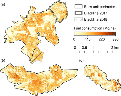
We quantified fuel consumption for canopy, shrub/seedling, herbaceous, DWD, litter, duff, total fuel, subcanopy fuel, and ACF. Consumption maps of total fuel are shown for each burn unit in Fig. 2. All consumption and fuel loading data for each burn unit are available on the WIFIRE Commons archive site: https://wifire-data.sdsc.edu/dataset/fuel-load-and-consumption-for-the-2017-2020-monroe-mountain-prescribed-fires.
Mapped estimates (10 m resolution) of total fuel consumed at the (a) Manning Creek (MCU) and adjacent blackline units, (b) Langdon Mountain (LMU) and (c) Annabella Reservoir (ARU) burn units using ALS-derived predictions.
The RF models with the highest variance explained (63.5–76.0%; Table 1) were those for the overstory (canopy fuel, ACF, and total fuel). Models for shrub/seedling and herbaceous fuels performed poorly, having 7.0 and 10.4% variance explained. Due to this, we omitted these from the results except if included in the aggregated fuel response variables (i.e. subcanopy fuel and total fuel). Shrub/seedling and herbaceous fuels comprised 3.3 and 0.2% of subcanopy fuels, respectively, and 1.1 and 0.01% of total fuels. The percentage variance explained for the other subcanopy fuels ranged from 25.6 to 42.9% (Table 1).
| Fuel type | % Var. Exp. | RMSE (Mg ha−1) | MBE (Mg ha−1) | |||||||||||
|---|---|---|---|---|---|---|---|---|---|---|---|---|---|---|
| RF | Consumption | Consumption | Consumption | Consumption | Consumption | Consumption | ||||||||
| Model | Geog. CV | 3-fold CV | Geog. CV | 3-fold CV | ||||||||||
| Canopy | 76.0 | 25.9 | (78.3%) | 26.2 | (81.1%) | 18.4 | (52.0%) | −6.0 | (−18.3%) | −7.2 | (−32.9%) | −4.6 | (−12.8%) | |
| DWD | 33.9 | 43.4 | (86.5%) | 49.4 | (91.2%) | 34.8 | (77.7%) | −17.6 | (−35.1%) | −29.6 | (−47.5%) | −12.4 | (−27.4%) | |
| Litter | 42.9 | 2.2 | (84.1%) | 2.9 | (103.2%) | 2.2 | (74.9%) | −0.6 | (−24.1%) | −1.8 | (−41.8%) | −0.8 | (−27.7%) | |
| Duff | 25.6 | 41.5 | (102.3%) | 55.5 | (114.2%) | 36.9 | (92.0%) | −15.0 | (−37.1%) | −36.1 | (−44.4%) | −11.9 | (−29.0%) | |
| Total fuel | 64.9 | 76.6 | (58.9%) | 98.6 | (70.9%) | 61.2 | (48.4%) | −31.3 | (−24.1%) | −64.8 | (−39.0%) | −23.8 | (−18.7%) | |
| Subcanopy fuel | 31.4 | 82.8 | (85.3%) | 102.3 | (90.3%) | 63.5 | (70.0%) | −37.8 | (−39.0%) | −74.3 | (−53.0%) | −27.3 | (−29.8%) | |
| ACF | 73.7 | 3.0 | (42.9%) | 3.4 | (64.7%) | 2.5 | (36.2%) | −1.4 | (−20.4%) | −1.9 | (−36.6%) | −1.3 | (−18.1%) | |
DWD, Down woody debris; ACF, Available canopy fuel.
The models for canopy fuel, total fuel, and ACF produced the lowest relative RMSE values (42.9–78.3%) and lowest absolute MBE values (i.e. closest to zero; −18.3 to 29.8%; Table 1) when comparing estimated and observed consumption for the entire set of plots. MBE values were consistently negative, indicating an underprediction bias. RMSE and MBE statistics from the random 3-fold cross-validation were better than using the entire set of plots, with 12.4% lower %RMSE and 4.9% lower %MBE on average across the fuel types (Table 1). Regarding the geographic cross-validation, to see how well the models could predict outside of the area they were trained in, all models had higher %RMSE (11.0% on average) and %MBE values (13.9% on average; Table 1). On average, the %RMSE were 23.5% higher and %MBE were 18.8% higher than for the random 3-fold cross-validation. This indicated RF models for all fuel types had greater error in predicting consumption when applied to a new area. However, canopy fuel, total fuel, and ACF tended to perform better in comparison to the other fuel types.
Discussion
Fuel consumption is intrinsically related to fire behaviour, heat release, plume dynamics, and smoke chemistry (Ottmar 2014; Van Der Werf et al. 2017; Prichard et al. 2019). At MCU, LMU, and/or ARU, data were collected on fire behaviour using in-situ sensors, plume dynamics using Doppler lidar, smoke composition and dispersion from UAS, aspen regeneration, and soil heating (Ottmar et al. 2021; Kobziar et al. 2024; Lareau et al. 2024). The intersection of these data provides a valuable nexus for advancing fire science toward understanding multiple disciplines cohesively. Within this context, it is important to understand the quality and the limitations of the fuel consumption estimates we developed.
Fuel consumption
Canopy fuel variables (i.e. canopy fuel, total fuel, and ACF) had the best model performance (highest pseudo-R2) and were most precise (lowest %RMSE) and accurate (lowest absolute %MBE) upon validation (Table 1). Others have also demonstrated that ALS data is less accurate when modelling subcanopy variables due to canopy occlusion and inability to directly capture the depth of some variables such as litter and duff (Bright et al. 2022; McCarley et al. 2022). Our models for DWD, litter, duff, and subcanopy fuel explained between 25.6 and 42.9% of variance. A review of literature on predicting subcanopy fuels from ALS data by Bright et al. (2022) found the range of variance explained to be 14–71%, suggesting our results are typical. Our model explained between 64.9 and 76.0% variance in total fuel, ACF, and canopy fuel. This is also typical in literature, with others demonstrating better fitting models of canopy than subcanopy fuels (Price and Gordon 2016; McCarley et al. 2020; Mauro et al. 2021). It follows that the models for subcanopy fuels performed worse when validating fuel consumption (Table 1). Therefore, users of the data we generated should know that there are potentially greater errors in the fuel consumption estimates for DWD, litter, duff, and subcanopy fuel.
For maximising accuracy and incorporating subcanopy fuels, estimates of total fuel were best. In validating total fuel consumption, it had the second lowest %RMSE and the third lowest absolute %MBE, behind canopy fuel and ACF (Table 1). The total fuel model likely had higher relative accuracy because of the stronger statistical relationship between ALS data and overstory canopy, as discussed previously, and the ecological relationship between the canopy and subcanopy, which has been demonstrated by others (e.g. Lydersen et al. 2015; Cansler et al. 2019).
Spatial transferability
In comparing consumption modelled from the full set of plots with the geographic cross-validation, the lower RMSE and MBE indicated that spatial transferability would result in loss of precision and accuracy. That is, parameters from RF models trained in a certain area are likely to result in poorer predictions when applied to a novel area without coincident fuel measurements on the ground. However, the extent to which model performance suffers was demonstrated to vary by fuel component (Table 1). There may be cases where some loss of predictive accuracy is an acceptable trade-off to acquiring field data.
A notable complication in our results is that the sample design of the plots in our study was opportunistic from a safety and logistics standpoint but not well-designed to capture the range of forest conditions in each unit. The clustered design (Fig. 1) introduced spatial autocorrelation, limiting the true independence of the observations. When we removed plots from the models at random, the statistics for consumption were better than if all plots for a given burn unit were removed. Such a problem may lead to worse out-of-sample predictions when observation independence is further reduced, as we observed in our geographic cross-validation. In this respect, our results are not a robust test of spatial transferability, but they emphasise the need for an unbiased and spatially representative sampling design, in which (1) sample plot locations are well distributed spatially and (2) each fuel condition is sampled in proportion to its occurrence on the landscape (Goodbody et al. 2023), in future efforts to develop generalised models of fuel consumption.
Fekety et al. (2018) performed a similar geographic cross-validation analysis to test the spatial transferability of lidar-trained RF models to predict basal area and stem density. They concluded that making RF model predictions onto a novel area without training data and within the same ecoregion was feasible but would likely result in greater errors than if training data were added to the novel area. Mauro et al. (2021) explored the potential for spatial transferability across multiple ALS datasets, finding that ecosystem differences and modelling techniques affected performance the most. Tompalski et al. (2019) showed average RMSE and MBE increased by as much as 29.31 and 22.04%, respectively, when ALS models were transferred to a new area. Similarly, we found an average increase in RMSE of 11.0% and MBE of 13.9%. These findings demonstrate the limitations of spatial transferability in developing generalised models and reinforce the importance of capturing the range of biophysical conditions in the training data to achieve the most accurate predictions.
Conclusions
We produced fuel consumption maps on three stand-replacing prescribed fires and two blackline units for canopy, DWD, litter, duff, total fuel, subcanopy fuel, and ACF. These data are available on WIFIRE Commons (see Data Availability Statement) and can be particularly useful to researchers who collected coincident fire behaviour, effects, and emissions data on the same fires. The precision and accuracy of these data vary, with canopy, total fuel, and ACF demonstrating the best performance. However, other predicted variables may be useful as they are the best available data for fuel consumption on these prescribed fires. Given ongoing FASMEE interest in future stand-replacing prescribed fires on the Fishlake National Forest, these models may be used to predict fuel consumption where pre- and post-fire ALS data are available, but ground data are not. Our results suggest reduced precision and accuracy from a spatially transferred model, so the tolerance for error in this approach should be considered against the cost of acquiring additional ground data for model refinement.
Data availability
Mapped estimates of fuel loads and consumption produced in this study are available on the WIFIRE Commons archive site: https://wifire-data.sdsc.edu/dataset/fuel-load-and-consumption-for-the-2017-2020-monroe-mountain-prescribed-fires. Field plot measurements used to train the predictive fuel models are available on the USDA Forest Service Research Data Archive at https://doi.org/10.2737/RDS-2024-0049. Links to these and related datasets can be found on the NASA LARC FireSense/FAMSEE data archive at https://www-air.larc.nasa.gov/missions/firesense/index.html.
Conflicts of interest
Andrew T. Hudak is an Associate Editor of International Journal of Wildland Fire. To mitigate this potential conflict of interest he had no editor-level access to this manuscript during the peer review. The authors declare no other conflicts of interest.
Declaration of funding
Data collection was funded by the Joint Fire Science Program’s Fire and Smoke Model Evaluation Experiment (FASMEE; Project 15-S-01-01) and the USFS Rocky Mountain Research Station (RMRS). Data analysis was funded via Joint Venture Agreements 17-JV-166 and 19-JV-165 between RMRS and the University of Idaho.
Acknowledgements
We thank the Fishlake National Forest for conducting the prescribed fire and allowing research crews access to these fires. We also thank everyone on the Fire and Environmental Research Applications Team (FERA) who collected field data.
References
Alonso-Rego C, Arellano-Pérez S, Guerra-Hernández J, Molina-Valero JA, Martínez-Calvo A, Pérez-Cruzado C, Castedo-Dorado F, González-Ferreiro E, Álvarez-González JG, Ruiz-González AD (2021) Estimating Stand and Fire-Related Surface and Canopy Fuel Variables in Pine Stands Using Low-Density Airborne and Single-Scan Terrestrial Laser Scanning Data. Remote Sensing 13(24), 5170.
| Crossref | Google Scholar |
Andersen HE, McGaughey RJ, Reutebuch SE (2005) Estimating forest canopy fuel parameters using LIDAR data. Remote Sensing of Environment 94(4), 441-449.
| Crossref | Google Scholar |
Bright BC, Hudak AT, McCarley TR, Spannuth A, Sánchez-López N, Ottmar RD, Soja AJ (2022) Multitemporal lidar captures heterogeneity in fuel loads and consumption on the Kaibab Plateau. Fire Ecology 18(1), 18.
| Crossref | Google Scholar | PubMed |
Cansler CA, Swanson ME, Furniss TJ, Larson AJ, Lutz JA (2019) Fuel dynamics after reintroduced fire in an old-growth Sierra Nevada mixed-conifer forest. Fire Ecology 15(1), 16.
| Crossref | Google Scholar |
Chuvieco E, Aguado I, Salas J, García M, Yebra M, Oliva P (2020) Satellite remote sensing contributions to wildland fire science and management. Current Forestry Reports 6(2), 81-96.
| Crossref | Google Scholar |
DRIScience (2020) Fire and Smoke Model Evaluation Experiment (FASMEE) – Overview. Available at https://youtube/Lo4Z6Qshtww?si=RJI0MdG3lP51xSNw [verified 30 March 2024]
Fekety PA, Falkowski MJ, Hudak AT, Jain TB, Evans JS (2018) Transferability of Lidar-derived Basal Area and Stem Density Models within a Northern Idaho Ecoregion. Canadian Journal of Remote Sensing 44(2), 131-143.
| Crossref | Google Scholar |
Goodbody TRH, Coops NC, Queinnec M, White JC, Tompalski P, Hudak AT, Auty D, Valbuena R, LeBoeuf A, Sinclair I, McCartney G, Prieur J-F, Woods ME (2023) sgsR: a structurally guided sampling toolbox for LiDAR-based forest inventories. Forestry 96, 411-424.
| Crossref | Google Scholar |
Hudak AT, Kato A, Bright BC, Loudermilk EL, Hawley C, Restaino JC, Ottmar RD, Prata GA, Cabo C, Prichard SJ, Rowell EM, Weise DR (2020) Towards Spatially Explicit Quantification of Pre- and Postfire Fuels and Fuel Consumption from Traditional and Point Cloud Measurements. Forest Science 66(4), 428-442.
| Crossref | Google Scholar |
Isenburg M (2013) LAStools - Efficient tools for LiDAR processing. Available at http://lastools.org
Keane RE, Herynk JM, Toney C, Urbanski SP, Lutes DC, Ottmar RD (2013) Evaluating the performance and mapping of three fuel classification systems using Forest Inventory and Analysis surface fuel measurements. Forest Ecology and Management 305, 248-263.
| Crossref | Google Scholar |
Kobziar LN, Lampman P, Tohidi A, Kochanski A, Cervantes A, Hudak A, McCarley R, Gullett B, Aurell J, Moore R, Vuono D, Christner BC, Watts AC, Cronan J, Ottmar R (2024) Bacterial emission factors: a foundation for the terrestrial-atmospheric modeling of bacteria aerosolized by wildland fires. Environmental Science and Technology 58(5), 2413-2422.
| Crossref | Google Scholar | PubMed |
Lareau NP, Clements CB, Kochanski A, Aydell T, Hudak AT, McCarley TR, Ottmar R (2024) Observations of a rotating pyroconvective wildland fire plume. International Journal of Wildland Fire 33, WF23045.
| Crossref | Google Scholar |
Lydersen JM, Collins BM, Knapp EE, Roller GB, Stephens S (2015) Relating fuel loads to overstorey structure and composition in a fire-excluded Sierra Nevada mixed conifer forest. International Journal of Wildland Fire 24(4), 484-494.
| Crossref | Google Scholar |
Mauro F, Hudak AT, Fekety PA, Frank B, Temesgen H, Bell DM, Gregory MJ, McCarley TR (2021) Regional modeling of forest fuels and structural attributes using airborne laser scanning data in Oregon. Remote Sensing 13(2), 261.
| Crossref | Google Scholar |
McCarley TR, Hudak AT, Sparks AM, Vaillant NM, Meddens AJH, Trader L, Mauro F, Kreitler J, Boschetti L (2020) Estimating wildfire fuel consumption with multitemporal airborne laser scanning data and demonstrating linkage with MODIS-derived fire radiative energy. Remote Sensing of Environment 251, 112114.
| Crossref | Google Scholar |
McCarley TR, Hudak AT, Restaino JC, Billmire M, French NHF, Ottmar RD, Hass B, Zarzana K, Goulden T, Volkamer R (2022) A comparison of multitemporal airborne laser scanning data and the fuel characteristics classification system for estimating fuel load and consumption. Journal of Geophysical Research: Biogeosciences 127(5), 1-17.
| Crossref | Google Scholar |
Ottmar RD (2014) Wildland fire emissions, carbon, and climate: modeling fuel consumption. Forest Ecology and Management 317, 41-50.
| Crossref | Google Scholar |
Ottmar RD, Sandberg DV, Riccardi CL, Prichard SJ (2007) An overview of the Fuel Characteristic Classification System – quantifying, classifying, and creating fuelbeds for resource planning. Canadian Journal of Forest Research 37(12), 2383-2393.
| Crossref | Google Scholar |
Ottmar R, Watts A, Larkin S, Brown T, French N (2021) Fire and Smoke Model Evaluation Experiment (FASMEE) Final Report—Phase 2. Joint Fire Sciences Program Project 15-S-01-01. 58 p. Available at https://research.fs.usda.gov/pnw/understory/fire-and-smoke-model-evaluation-experiment-final-report-phase-2
Peterson DL, Hardy CC (2016) The RxCADRE study: a new approach to interdisciplinary fire research. International Journal of Wildland Fire 25(1), i.
| Crossref | Google Scholar |
Price OF, Gordon CE (2016) The potential for LiDAR technology to map fire fuel hazard over large areas of Australian forest. Journal of Environmental Management 181, 663-673.
| Crossref | Google Scholar | PubMed |
Prichard SJ, Kennedy MC, Wright CS, Cronan JB, Ottmar RD (2017) Predicting forest floor and woody fuel consumption from prescribed burns in southern and western pine ecosystems of the United States. Forest Ecology and Management 405, 328-338.
| Crossref | Google Scholar |
Prichard SJ, Larkin N, Ottmar R, French N, Baker K, Brown T, Clements C, Dickinson M, Hudak A, Kochanski A, Linn R, Liu Y, Potter B, Mell W, Tanzer D, Urbanski S, Watts A (2019) The fire and smoke model evaluation experiment—a plan for integrated, large fire–atmosphere field campaigns. Atmosphere 10(2), 66.
| Crossref | Google Scholar | PubMed |
Riccardi CL, Ottmar RD, Sandberg DV, Andreu A, Elman E, Kopper K, Long J (2007) The fuelbed: a key element of the fuel characteristic classification system. Canadian Journal of Forest Research 37(12), 2394-2412.
| Crossref | Google Scholar |
Skowronski NS, Clark KL, Duveneck M, Hom J (2011) Three-dimensional canopy fuel loading predicted using upward and downward sensing LiDAR systems. Remote Sensing of Environment 115(2), 703-714.
| Crossref | Google Scholar |
Stefanidou A, Gitas IZ, Korhonen L, Georgopoulos N, Stavrakoudis D (2020) Multispectral LiDAR-Based estimation of surface fuel load in a dense coniferous forest. Remote Sensing 12(20), 3333.
| Crossref | Google Scholar |
Taneja R, Hilton J, Wallace L, Reinke K, Jones S (2021) Effect of fuel spatial resolution on predictive wildfire models. International Journal of Wildland Fire 30(10), 776-789.
| Crossref | Google Scholar |
Tompalski P, White JC, Coops NC, Wulder MA (2019) Demonstrating the transferability of forest inventory attribute models derived using airborne laser scanning data. Remote Sensing of Environment 227, 110-124.
| Crossref | Google Scholar |
Van Der Werf GR, Randerson JT, Giglio L, van Leeuwen TT, Chen Y, Rogers BM, Mu M, van Marle MJE, Morton DC, Collatz GJ, Yokelson RJ, Kasibhatla PS (2017) Global fire emissions estimates during 1997-2016. Earth System Science Data 9(2), 697-720.
| Crossref | Google Scholar |