

Spatial variability of soil carbon across a hillslope restoration planting in New Zealand
Molly Katharine D’Ath A , Katarzyna Sila-Nowicka A * and Luitgard Schwendenmann A
A
Abstract
Forest restoration has been adopted by governments and local communities across the globe to restore ecological functions and as a measure to mitigate climate change.
This study investigated the spatial variation in landscape, vegetation, soil characteristics, and soil carbon storage under young restoration plantings across a hillslope in northern New Zealand.
Soil samples (0–10 cm, 10–20 cm, and 20–30 cm) were taken from 121 locations across 5–20-year-old restoration plantings, remnant and regenerating bush and pasture. Samples were analysed for bulk density, pH, and soil carbon concentration and soil carbon stocks were calculated. Ordinary kriging and multiscale geographically weighted regression (MGWR) were used to predict and explain soil carbon stocks across the landscape.
Soil carbon stocks (0–10 cm depth) across the study area ranged from 1.9 to 7.1 kg m−2. Spatial analysis revealed that elevation, slope, stem density, bulk density, and pH had a significant effect on the magnitude and distribution of soil carbon stocks.
This study has shown that topography had a strong effect on soil carbon stocks across the young restoration plantings. The outcome of this study highlights the importance of taking landscape and soil characteristics into account when planning a forest restoration project.
Keywords: geographically weighted regression, land cover change, landscape, native vegetation, reforestation, soil carbon, spatial analysis, topography.
Introduction
Ecological restoration is a common practice globally. Restoration aims to assist the recovery of an ecosystem that has been degraded by reintroducing species or the modification of physical conditions (Society for Ecological Restoration International Science & Policy Working Group 2004; Martin 2017). Restoration can increase biodiversity as well as ecosystem services (Benayas et al. 2009; Mori 2017; Chazdon and Brancalion 2019). One of these ecosystem services is carbon sequestration, which is considered an important land-based mitigation tool for offsetting carbon emissions (Harper et al. 2018; Messier et al. 2021).
Soil plays a key role in the functioning of terrestrial ecosystems, such as water filtration and nutrient cycling (Adhikari and Hartemink 2016). An example of climate regulation is soil carbon sequestration through organic matter breakdown and storage (Stockmann et al. 2013; Baldocchi and Penuelas 2019). Soil carbon sequestration and storage are influenced by current and past land use and climate (Stockmann et al. 2013; Wiesmeier et al. 2019). Soil carbon storage is affected by changes in vegetation cover resulting in a modification of organic matter input and subsequently soil carbon (Kirschbaum et al. 2013; Sulman et al. 2020). Topography also plays a major role in driving the spatial variability of soil properties, including soil carbon (Wiesmeier et al. 2019; Adhikari et al. 2020). For example, slope gradient and aspect influence soil temperature and soil moisture, which affects productivity and organic matter decomposition rates (Griffiths et al. 2009; Lozano-García et al. 2019). The quality and quantity of soil carbon are also influenced by elevation, given the negative correlation between elevation and temperature, leading to reduced rates of organic matter decomposition (Saeed et al. 2019). Further, the loss of soil carbon and nutrients through erosion has been related to topography (Berhe et al. 2007).
Forest restoration often occurs on degraded agricultural land and marginal land (e.g. hillslopes) (Trotter et al. 2005). Soil characteristics are spatially variable, especially in hill country with slopes >15% (Morton et al. 2000; Hedley et al. 2013). Investigating the spatial distribution of soil characteristics is critical in determining soil functions and to inform land use management, in particular on hillslopes (Stutter et al. 2009; Barrena-González et al. 2023). Mapping and predicting spatial patterns of soil characteristics can be achieved using a wide range of spatial interpolation methods (Zhang et al. 2020).
The majority of the studies investigating the relationship between soil carbon stocks and environmental factors have used traditional statistical analysis, which can only produce global (average) parameter estimates and ignoring the spatial variation in these relationships (Mirchooli et al. 2020). The most common global method is a global regression, which reports reasonably good performance for predicting carbon stocks using climate and socio-economic conditions (housing age, income or population density) as predictors (Song et al. 2018, Contosta et al. 2020). An improvement on simple regression is kriging regression that combines regression with kriging for spatial interpolation by predicting the dependent variable based on environmental covariates and adjusting for prediction residuals (Zhu et al. 2022). Due to potential nonlinear relationship between soil carbon stocks and environmental factors random forest models have been found useful for soil carbon prediction (Song et al. 2018). Despite significant progress in these methods, there are many challenges, especially in uncovering the varying spatial relationships in highly variable, topographically challenging, and complex landscapes. By using spatial regression models such as geographically weighted (Jensen et al. 2018) regression (GWR) or recently developed, more complex multiscale GWR (MGWR), researchers have been able to model spatial variability of carbon and soil characteristics more accurately by weighting topographical and environmental variables at different locations (Kumar et al. 2013; Costa et al. 2018; Song et al. 2018; Gao et al. 2021; Lin et al. 2024).
Studies have been done on the above- and below-ground carbon storage in restoration plantings (Schwendenmann and Mitchell 2014; Kimberley et al. 2021) and regenerating shrublands (Trotter et al. 2005; Carswell et al. 2012; Mason et al. 2014) in New Zealand. However, research on the spatial variation in soil carbon stocks and the relationships between soil, vegetation, and landscape characteristics in young restoration plantings in New Zealand is lacking. The objectives of this study were to (1) determine vegetation and soil characteristics affecting carbon stocks, (2) quantify soil carbon stocks (to 30 cm depth), and (3) map the spatial distribution of vegetation and soil characteristics. We also investigated the effects of vegetation, landscape, and soil characteristics on soil carbon stocks using ordinary kriging interpolation and MGWR models.
Materials and methods
Study area
The study was carried out near Glorit (174.4530E, 36.4921S; 174.4587E, 36.4950S), Auckland, New Zealand (Fig. 1). The 24-ha study site is classified as undulated medium hill area. The elevation ranges from 20 to 136 m above sea level with slopes reaching 20 degrees. The region where the site is located features a warm subtropical climate, with annual rainfall of 1457.5 mm and mean annual temperature of 14–16°C (Chappell 2014). The geology of the study site is late quaternary alluvium and colluvium, which consists of unconsolidated to poorly consolidated sand, gravel, mud, and peat. This overlies the early Miocene Waitemata group, which consists of interbedded sandstone and mudstone (Ballance and McCarthy 1975). The soil types of this area are classified as mottled and typic yellow ultic soils (Hewitt 2010).
Map showing the location of the study area (outlined in red), Kaipara Harbour, Rodney District, North Island, New Zealand.
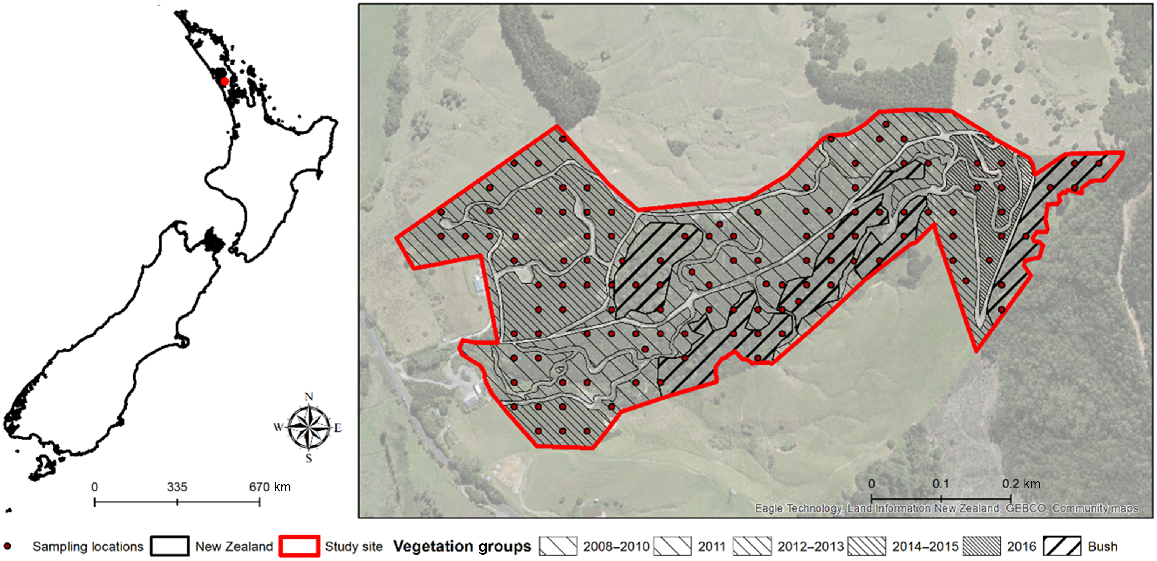
During the late 19th and early 20th century, most of the dense forest and bush was cleared and converted into pasture (Beever 1981). Some areas of remnant bush remained and there are patches of naturally regenerating bush across the hillslope (Noble and Harmsworth 1990). In 2008 restoration work began and native species were planted annually until 2016.
Sampling design
The 121-sample points were chosen to adhere to budget and time constraints. A combination of systematic and judgemental sampling was used to generate sample points across the study area (Fig. 1). Systematic sampling based on a uniform grid was initially used, as it is preferable for spatial analysis. However, judgemental sampling, refined from a stratified random method was incorporated. This adjustment was necessary because certain vegetation groups were not adequately covered with sample points using systematic sampling alone (Lark and Marchant 2018), or roads hindered systematic coverage of the study site. The study area was divided into seven different vegetation groups (Fig. 1). The vegetation groups were pasture (sample points = 3); plantings between 2008 and 2010 (sample points = 18), 2011 (sample points = 13), 2012–2013 (sample points = 17), 2014–2015 (sample points = 35), 2016 (sample points = 6) and a reference group of bush (sample points = 29) that included the remnant bush and naturally regenerating bush present in the study area.
Vegetation survey and soil sampling
A vegetation survey was conducted at each sample point using the Point-Centred Quarter (PCQ) method (Mitchell 2010). Organic layer (forest floor) samples were taken using a PVC ring (diameter, 10 cm; length, 8 cm) at 121 locations. Mineral soil samples (one sample for bulk density and one sample for soil physical and chemical analysis) were collected using a soil auger (diameter, 3.5 cm). At 0–10 cm depth, samples were taken at all 121 locations, at 10–20 cm, samples were taken at 50 locations, and at 20–30 cm, samples were taken at 25 locations. Field measurements and sampling were conducted between October and December 2019.
Laboratory analysis
Organic layer samples were oven dried at 60°C for 1 week and then weighed to determine the organic layer biomass. Mineral soil samples for bulk density analysis were dried at 105°C for 1 week. The soil weight (oven dry) was divided by the moist volume to obtain bulk density (Blakemore et al. 1987). Mineral soil samples for physical and chemical analyses were dried at 40°C for 1 week (McKenzie 2000). Roots and organic matter were removed, and the soil was sieved through a 2-mm sieve. For particle size analysis 20 mL of 0.55% Calgon deflocculant solution was added to 10 g of soil. The soil–Calgon mix was analysed using a laser particle size analyser (Mastersizer 3000, Malvern Panalytical, Worcestershire, UK). For pH, 25 mL of deionised water was added to 10 g mineral soil and measured using a pH electrode (sensION + PH3, HACH, Loveland, CO, USA).
Accurate and precise determination of soil carbon concentration can be obtained by automated, high-temperature dry combustion methods (Chatterjee et al. 2009). Due to financial constraints and instrument availability, we were only able to analyse a subset of mineral soil samples (n = 66) by high-temperature dry combustion. The oven-dried (<2 mm) samples were ground into powder using a centrifugal mill (ZM 300, Retsch GmbH, Haan, Germany). Total carbon concentration was determined by weighing 10 mg of ground material into tin cups and combusting the sample at 950°C using an elemental analyser (Vario El Cube Elementar, Langenselbold, Germany). Of these, 10% of samples were measured twice. The variability was <1%.
Loss on ignition (LOI) is a cheaper method to estimate organic matter content from which the total carbon concentration can be calculated using a conversion factor. When LOI and total carbon concentrations are both measured, regression models are used to convert LOI to soil carbon concentration (Jensen et al. 2018). We determined organic matter in all mineral soil samples by LOI following the method described by Blakemore et al. (1987). Five grams of oven-dry (40°C) soil was placed into previously ignited and weighed porcelain crucibles, dried at 105°C for 24 h, cooled in a desiccator and weighed again. Finally, the crucibles were ignited at 500°C for 4 h in a muffle furnace (Elecfurn, The Electric Furnace Co Ltd, Auckland, New Zealand). After ignition, the crucibles were cooled in a desiccator and weighed. The organic matter content was calculated as the difference between the oven-dry (105°C) weight before and after ignition.
A linear regression function was established between organic matter content and total carbon concentration (r2 = 0.88; P < 0.001). This function was used to estimate total carbon concentration for the remaining mineral soil samples. The pH values (median = 5.3) suggest an insignificant amount of inorganic (carbonate) carbon. Thus, total carbon concentration is a good reflection of soil organic carbon in this study area. Soil carbon stocks (kg m−2) were calculated using the estimated total carbon concentration (g kg−1 soil), bulk density (kg m−3), and sampling depth (m).
Landscape variables
To calculate elevation, slope, and aspect, we used an 8-m Digital Elevation Model (LINZ 2023a). The road and river centrelines, essential for distance calculations concerning paths and water bodies, were sourced from the NZ Road/Rivers Centrelines dataset (Topo, 1:250 k) (LINZ 2023b). To ensure precision in distance measurements, we generated Euclidean distance surfaces. The Euclidean distance surface illustrates the distance from each raster cell to a source or a set of sources (rivers, roads) based on straight-line distance.
Statistical analysis
Shapiro-Wilk’s test was used to test if the data was normally distributed (Shapiro and Wilk 1965). As some soil characteristics were non-normally distributed, a Kruskal–Wallis test was used to identify if there were significant differences in soil characteristics between vegetation groups at P < 0.05 (Kruskal and Wallis 1952). A post hoc Wilcoxon test was then run to identify which vegetation groups were significantly different. Statistical tests were carried out using R (R Core Team 2021).
Spatial analysis
Spatial interpolation and MGWR methods were used to predict the spatial distribution of soil carbon stocks (0–10 cm, 10–20 cm, and 20–30 cm) and to investigate the relationship between soil and vegetation characteristics and topographic features for the top layer of soil (0–10 cm). The outline of the analysis is in Fig. 2.
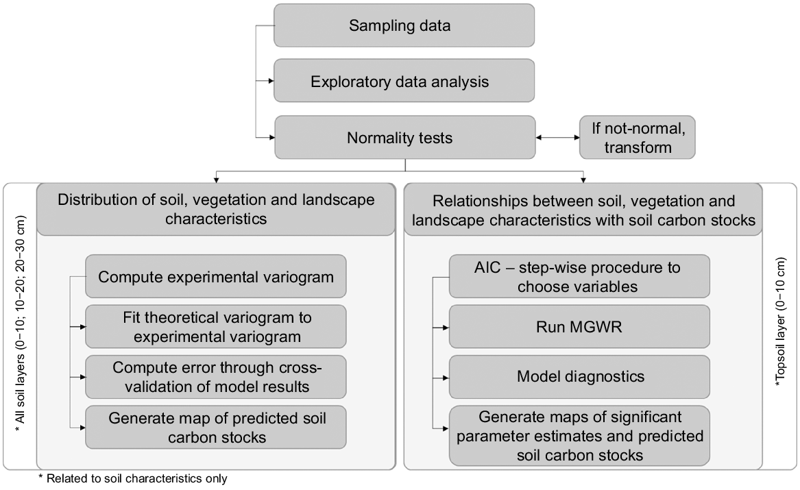
To understand the spatial distribution of soil carbon stocks, ordinary kriging was selected over other univariate geostatistical methods as this method accounts for local variation in a studied phenomenon and so predicts spatial trends in values of an attribute (Li and Heap 2011, 2014). The accuracy of this method is limited, because it uses a stationary mean within the local search window. To execute ordinary kriging, the spatial dependence of observations was specified through a variogram. An experimental variogram is determined directly from measurements of the characteristic, and the prediction of unsampled locations is then generated by fitting a theoretical variogram to the experimental variogram (Volfová and Šmejkal 2012). Theoretical variograms provide continuity so variance can be obtained at any distance, and follow various model forms (i.e. spherical, exponential, steady/stable). A variogram contains a sill, nugget, and range. The sill is the upper value of the variogram, the nugget is the value of the variogram where the distance is zero, and the range is the maximum distance at which two observations are dependent (Volfová and Šmejkal 2012). To assess how accurate the predicted values at unknown locations were, leave-one-out cross-validation was performed where one data point was held back from analysis and predicted using the data from all other locations. The predicted and the original values are then compared. This is then repeated with all data points to inform the quality of the model. One operation of cross-validation was calculating the root mean square error (RMSE). Spatial interpolation was carried out using ArcMap ver. 10.8 and variograms were generated using ‘gstat’ and ‘automap’ packages in R (Environmental Systems Research Institute 2020; R Core Team 2021; Himestra and Skoin 2023; Pebesma and Graeler 2023).
To explore the spatial variability in the relationships between soil carbon stocks and potential influencing factors, we employed a multiscale geographically weighted regression (MGWR) analysis.
A standard geographically weighted regression (GWR) represents a spatial statistical approach that surpasses conventional global regression models, which assume constant relationships across space. It achieves this by acknowledging the spatial heterogeneity in spatial processes, which delineates how these processes vary according to spatial context (Fotheringham et al. 1998; Oshan et al. 2019). In GWR, local linear models are established at multiple locations using data from the neighbourhoods surrounding these points within a specified spatial bandwidth. Multiscale geographically weighted regression considers the spatial coordinates of the observed phenomena and predicts parameter estimates based on weighted distances between these locations and a given regression point (Fotheringham et al. 2017). Moreover, MGWR extends beyond GWR by accounting for the spatial influence on the relationship between independent and dependent variables. It allows for the modelling of both local and global relationships for all variables within the model. In practical terms, MGWR computes separate regression models for every location within the dataset, and it calculates a corresponding bandwidth for each variable. This model can be formally expressed as:
where yi is a value of the dependent variable at i location, β0 is an intercept, βbwj is the bandwidth to calibrate the ith relationship, (ui, vi) is the spatial location of the ith observation, and ε is the random error term.
To enhance our understanding of the relationships between soil carbon stocks and various characteristics encompassing vegetation, soil, and site attributes, we employed a MGWR model. We systematically selected 13 exploratory variables, guided by the existing literature and data availability. Subsequently, we conducted a model selection procedure based on the Akaike Information Criterion (AIC) (Fotheringham et al. 2002). This rigorous process uses AIC values to identify suitable variables based on stepwise forward selection process. Observations revealed that after incorporating a total of 11 variables, the AIC values ceased decreasing with the addition of further variables. Consequently, the last two aspect-related variables were excluded from the final model. As the dependent variable we used soil carbon stocks from 121 sampling locations.
The MGWR was performed using a Python library developed by Oshan et al. (2019) and the results were visualised in ArcMap ver. 10.8.
Results and discussion
Landscape, vegetation, and soil characteristics
Stem density (0.1–2.9 trees m−2), stand basal area (0.2–645 m2 ha−1) and organic layer biomass (1–104 g m−2) varied considerably across the study area (Table 1).
| Min | Max | Mean | Median (LQ-UQ) | s.d. | ||
|---|---|---|---|---|---|---|
| Landscape and vegetation characteristics | ||||||
| Elevation (m) | 22.25 | 136.16 | 65.43 | 57.83 (40.69–89.85) | 29.73 | |
| Slope (°) | 1.61 | 19.62 | 10.16 | 10.13 (8.16–12.14) | 3.21 | |
| Distance to path (m) | 0.36 | 148.8 | 32.95 | 18.83 (11.96–49.27) | 29.9 | |
| Distance to waterway (m) | 0.26 | 148.8 | 36.39 | 28.38 (12.01–55.70) | 31.55 | |
| Stem density (n m−2) | 0.07 | 2.89 | 2.38 | 0.80 (0.42–1.23) | 0.8 | |
| Stand basal area (m2 ha−1) | 0.24 | 645.75 | 41.56 | 18.84 (8.63–33.37) | 91.94 | |
| Organic layer biomass (g m−2) | 0.38 | 104.09 | 16.61 | 7.30 (3.98–22.17) | 20.95 | |
| Mineral soil characteristics | ||||||
| 0–10 cm | ||||||
| Clay (%) | 2.5 | 17.14 | 8.5 | 8.48 (6.33–10.10) | 2.79 | |
| Silt (%) | 23.89 | 67.67 | 41.02 | 41.65 (36.23–46.62) | 7.51 | |
| Sand (%) | 15.16 | 71.73 | 50.3 | 49.47 (44.24–56.65) | 9.6 | |
| Bulk density (g cm−3) | 0.47 | 1.45 | 1.01 | 1.01 (0.88–1.12) | 0.18 | |
| pH | 4.55 | 6.87 | 5.34 | 5.32 (5.08–5.53) | 0.36 | |
| Total carbon (%) | 1.73 | 6.89 | 4.09 | 4.11 (3.07–5.03) | 1.15 | |
| 10–20 cm | ||||||
| Clay (%) | 6.32 | 20.41 | 12.33 | 12.33 (8.64–15.41) | 4.16 | |
| Silt (%) | 27.85 | 62.34 | 43.46 | 43.07 (37.56–49.90) | 8.62 | |
| Sand (%) | 17.25 | 64.78 | 44.22 | 43.32 (35.55–52.16) | 12.07 | |
| Bulk density (g cm−3) | 0.8 | 1.82 | 1.15 | 1.13 (0.99–1.82) | 0.23 | |
| pH | 4.55 | 6.25 | 5.3 | 5.28 (4.96–5.48) | 0.51 | |
| Total carbon (%) | 0.98 | 5.34 | 3.12 | 3.06 (2.50–3.73) | 0.89 | |
| 20–30 cm | ||||||
| Clay (%) | 7.01 | 27.11 | 17.35 | 17.12 (13.82–20.61) | 5.45 | |
| Silt (%) | 23.74 | 61.67 | 43.16 | 46.13 (36.94–50.25) | 9.95 | |
| Sand (%) | 11.22 | 69.25 | 39.04 | 36.16 (30.56–46.30) | 13.77 | |
| Bulk density (g cm−3) | 0.9 | 1.58 | 1.26 | 1.28 (1.17–1.58) | 0.17 | |
| pH | 4.61 | 5.74 | 5.01 | 5.01 (4.81–5.13) | 0.3 | |
| Total carbon (%) | 1.64 | 3.28 | 2.4 | 2.32 (2.19–2.59) | 0.48 | |
Min, minimum; max, maximum; LQ, lower quartile; UQ, upper quartile, s.d., standard deviation
The soil was sand and silt dominated and classified as loamy sand, sandy loam, and loamy silt. Median bulk density ranged between 1 and 1.3 g cm−3 and increased slightly with soil depth. Median pH at 0–10 cm and 10–20 cm was 5.3 and slightly lower at 20–30 cm (Table 1).
Soil carbon stocks at 0–10 cm varied between 1.9 and 7.1 kg m−2 (Fig. 3). Soil carbon stocks in the pasture was significantly higher than in restoration plantings and bush. Soil carbon stocks in the 2014–2015 plantings were higher than 2011. No difference in soil carbon stocks was found between the other vegetation groups. Carbon stocks at 10–20 cm depth ranged from 1.8 to 5.4 kg m−2, and in 20–30 cm depth from 2.3 to 4.4 kg m−2. There were no significant differences in soil carbon stocks between vegetation groups at 10–20 cm and 20–30 cm.
Soil carbon stocks (0–10 cm) across the vegetation groups. The horizontal line in the box indicates the median; the boundaries of the box represent the 25th and 75th percentile, and the whiskers show the highest and lowest values.
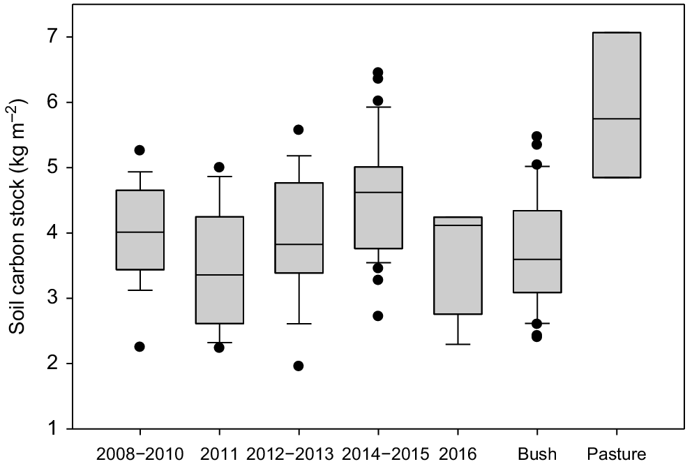
Soil carbon stocks found in the bush and pasture at Glorit were within the range found in New Zealand indigenous shrublands (3.2–4.6 kg m−2; Hedley et al. 2013) and pastures (3.7–6.7 kg m−2; Scott et al. 1999; Sparling and Schipper 2004). Soil carbon stocks varied considerably within a given layer but tended to decrease with depth (Fig. 4). A decrease in soil carbon stocks with depth has been reported in other studies and is partly explained by the decline in litter and root derived organic matter input with depth (Lawrence et al. 2015; Henneron et al. 2022).
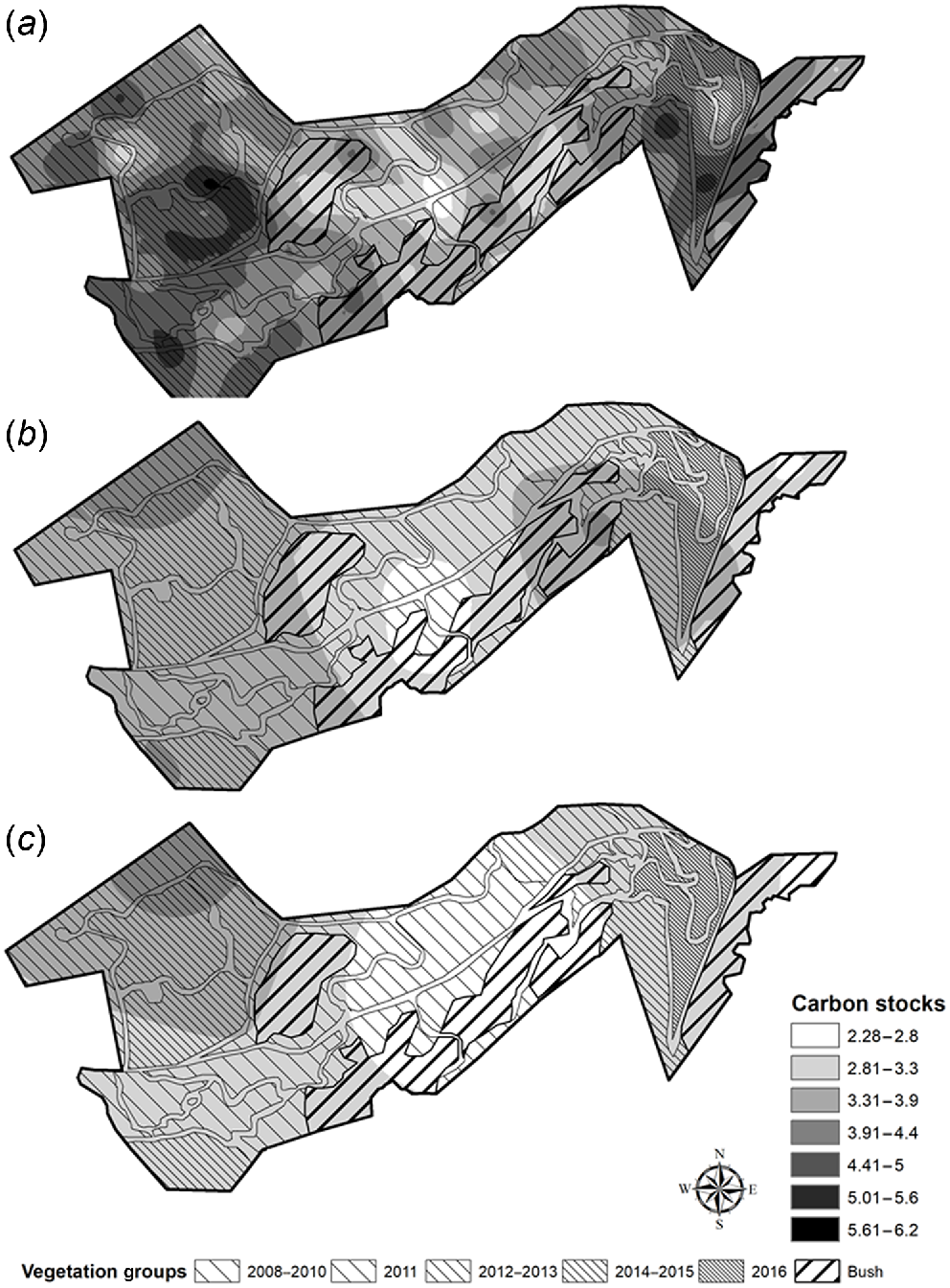
Ordinary kriging of soil carbon stocks (kg m−2) at different depths across the study area. (a) 0–10 cm, (b) 10–20 cm, and (c) 20–30 cm. Note that we did not map carbon stocks from pasture-related samples as we only had three sampling locations.
Soil carbon stocks (0–10 cm) in the restoration plantings were significantly lower compared to the pasture (Fig. 3). This is in line with previous findings (Guo and Gifford 2002; Guo et al. 2007) reporting a decrease in soil organic carbon following afforestation. The young age of the tree plantings may partly explain the lower carbon stocks in the restoration plantings (Guo and Gifford 2002). Another factor may be the initial carbon stock. An increase in soil carbon following afforestation often occurs in soils low in carbon, while a decrease has been found in carbon rich soils (Hong et al. 2020).
Ordinary kriging
We computed and fitted a variogram to assess the distribution of soil carbon stocks across various vegetation groups. Pasture samples were excluded from the analysis due to their limited number (three in total) and their spatial separation from the primary study site. The experimental variograms of soil carbon stocks (0–10 cm) had relatively weak trends, which can happen in complex terrain with numerous variables at play. The theoretical models fit the experimental variograms with the following parameters (model choice, steady; sill, 0.45; Nugget, 0.43; Range, 66.11).
The predicted surface of soil carbon stocks at 0–10 cm showed a small area of low values (2.5–2.8 kg m−2) at the centre of the study area (Fig. 4a). Higher values (4.4–6.2 kg m−2) were predicted at the south-western edge and the southern tip at the eastern end of the study area. The predicted surface of soil carbon stocks at 10–20 cm showed lower values (2.9–3.3 kg m−2) in the centre, and higher values (3.4–4.4 kg m−2) in the north-west of the study area (Fig. 4b). The prediction surface for this layer was smoother than that at 0–10 cm depth. At 20–30 cm low values (2.3–2.8 kg m−2) were again found in the centre of the study area and high values (4.0–4.4 kg m−2) were predicted in the north-western section of the study area (Fig. 4c).
Multiscale geographically weighted regression
Results derived from the calibrated MGWR model are in Table 2 and Fig. 5. Table 2 shows the final list of variables with ranges of parameter estimates as well as model’s diagnostics.
| Global regression | MGWR parameter estimates (all values) | ||||||
|---|---|---|---|---|---|---|---|
| Variables | Beta estimates | P-value | Min | Mean | Median | Max | |
| Elevation (m) | −0.426 | 0.049 | −0.678 | −0.421 | −0.354 | 0.467 | |
| Slope (°) | −0.258 | 0.036 | −0.298 | −0.281 | −0.257 | −0.226 | |
| Path proximity (m) | −0.134 | 0.547 | −0.189 | −0.072 | −0.124 | 0.004 | |
| Waterway proximity (m) | 0.210 | 0.303 | 0.143 | 0.280 | 0.240 | 0.735 | |
| Mean basal area (m2) | 0.160 | 0.549 | 0.025 | 0.137 | 0.089 | 0.342 | |
| Stand basal area (m2 ha−1) | 0.011 | 0.965 | −0.075 | 0.001 | 0.000 | 0.054 | |
| Stem density (n m−2) | 0.247 | 0.043 | −0.202 | 0.062 | −0.020 | 0.351 | |
| Sand (%) | −0.498 | 0.337 | −0.644 | −0.615 | −0.617 | −0.573 | |
| Silt (%) | −0.290 | 0.575 | −0.493 | −0.425 | −0.440 | −0.434 | |
| Bulk density (g cm−3) | 0.709 | 0.019 | 0.620 | 0.725 | 0.719 | 0.674 | |
| pH | 0.142 | 0.198 | 0.137 | 0.206 | 0.187 | 0.267 | |
| Model diagnostics | Global regression | MGWR | |
|---|---|---|---|
| R2 | 0.190 | 0.590 | |
| Adj R2 | 0.290 | 0.490 | |
| AIC | 250.690 | 230.150 |
Multiscale geographically weighted regression (MGWR) local parameter estimates for (a) elevation, (b) slope, (c) stem density, (d) bulk density, and (e) pH.
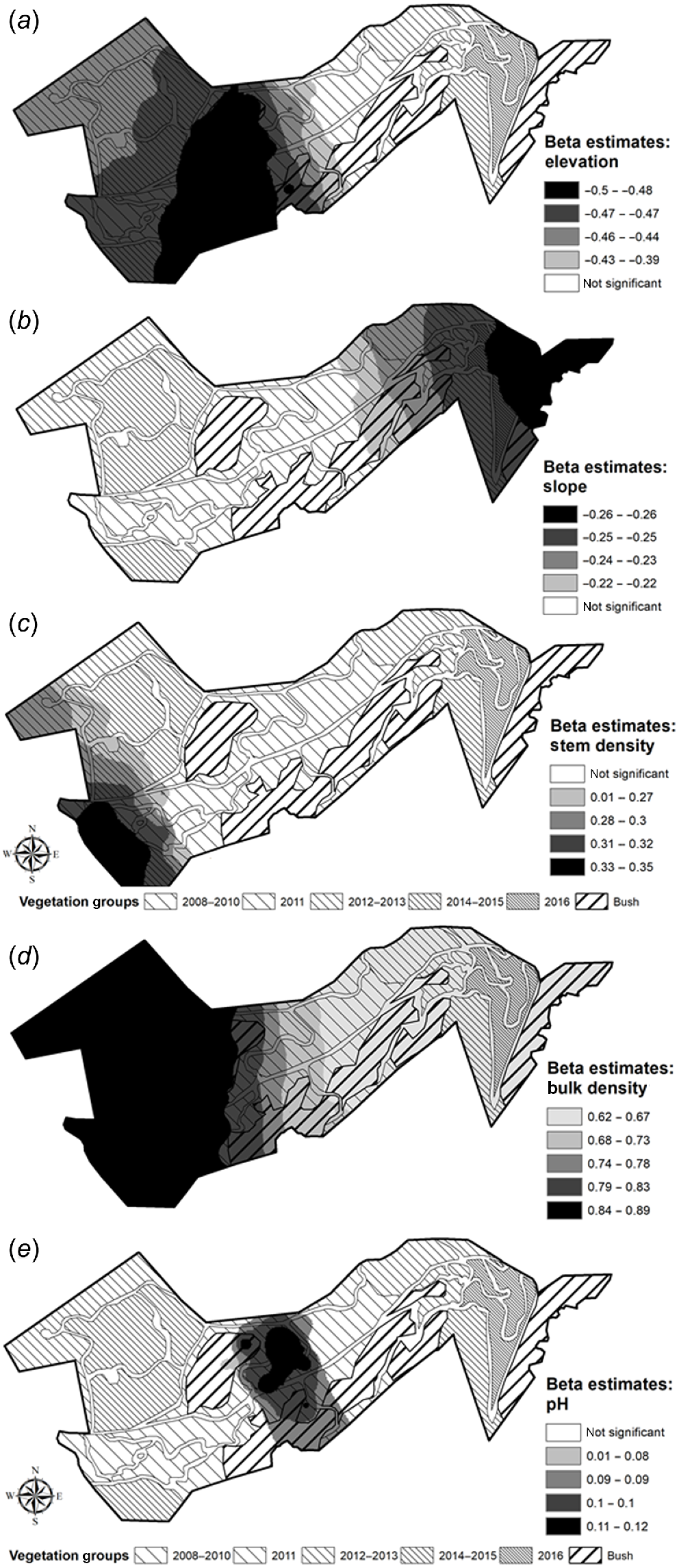
Fig. 5 shows five maps of local parameter estimates. Only local parameters that were significant were mapped. The global estimate demonstrated a statistically significant negative relationship (−0.426), signifying an inverse relationship between elevation and soil carbon stocks (Fig. 5a). This suggests that carbon stocks decreased with elevation, which can be attributed to slightly decreasing temperatures, resulting in reduced rates of organic matter decomposition (Saeed et al. 2019). This trend was particularly strong in the western site of the study area, characterised by lower elevation and situated at the base of the hill. Lower elevation in this study area coincided with comparatively low bulk density values and low basal area (see Supplementary Figs S1–S4), which may partly explain lower soil organic carbon stocks. The inverse distance interpolation (IDW) was chosen to map chemical, physical, and environmental parameters shown in supplementary materials. This method calculates value in a grid point while considering neighbouring locations within a user-defined search radius. IDW is commonly employed in soil investigations due to its ease of implementation (Li and Heap 2011, 2014; Zhang et al. 2020).
Fig. 5b illustrates the local parameter estimates concerning the association between soil carbon stocks and slope, accounting for variations in other variables within the model. The global parameter estimate for this relationship was −0.258, suggesting an overall negative influence of slope on soil carbon stocks. However, the results from the MGWR indicate spatial variability in the strength of these effects. Across most of the western and central portions of the study area, the parameters were statistically insignificant. In contrast, the eastern part showed a significant negative relationship, indicating that increasing slopes in this region corresponded to lower soil carbon stocks. A negative relationship between slope and soil carbon has been reported in previous studies and has been explained by soil erosion and water runoff washing organic material off steep slopes to lower elevations (Gregorich et al. 1998; Zhong et al. 2017).
Fig. 5c depicts the local parameter estimates relating to a vegetation characteristic, stem density. The global relationship was positive (0.247), suggesting that higher stem density has a positive influence on soil carbon stocks. These parameter estimates indicate spatial variation, with significance observed exclusively in the western area of the study site with older (2008–2010) and more recent plantings (2024–2025). Some of the restoration plantings contained patches of higher stem density (Figs S1–S4). This is similar to the results from Na et al. (2021) where they found that higher tree density resulted in higher soil carbon stocks.
Fig. 5d indicates the study area where bulk density (g cm−3) had a significant positive effect on soil carbon stocks. The global estimate was significantly positive (0.709). The significantly positive relationship was found across the whole study area, with a stronger effect in the western area of the study site where bulk density tended to be lower compared to the remaining area (Figs S1–S4). Given that soil carbon stocks are estimated using soil carbon concentration and bulk density, bulk density was the dominant driver in areas where soil carbon concentration was fairly homogenous as in the western part of the study area (Figs S1–S4).
Fig. 5e delineates the local relationships between pH and soil carbon stocks. Globally, this relationship was not significant (0.142). However, the results from MGWR indicate local variations, with a significant positive relationship between pH and soil carbon stocks observed in the central part of the study site. Some studies have reported a positive relationship between pH and soil carbon content (Kuśmierz et al. 2023). Higher pH have been shown to contribute to enhanced plant growth resulting in higher biomass and litter input (Malik et al. 2018).
Further, we used MGWR to predict levels of soil carbon stocks in the study area (Fig. 6). We used IDW to map the results as a continuous surface.
Multiscale geographically weighted regression (MGWR)-derived soil carbon stocks (0–10 cm). These predicted soil carbon stocks values were interpolated using IDW interpolation to produce this continuous surface.
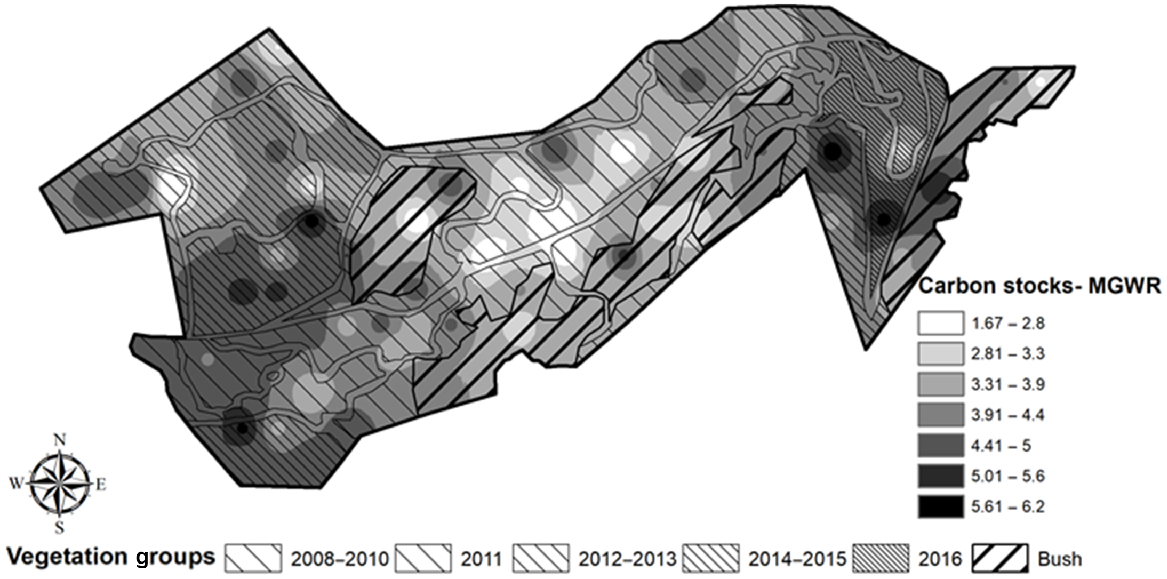
The MGWR-derived carbon stocks (Fig. 6) exhibit similar patterns to those derived from ordinary kriging (Fig. 4a). Predictions from MGWR reveal more detailed patterns with sharper boundaries for minimums and maximums. The fact that the predictions extend beyond the original values suggests that landscape and vegetation characteristics influence soil carbon stock levels. Typically, in flat areas, ordinary kriging may predict better due to accounting for spatial auto-correlation. However, in our case study, with a significant effect of elevation and slope, it is reasonable to assume that MGWR captures some variations more effectively (Wang et al. 2012).
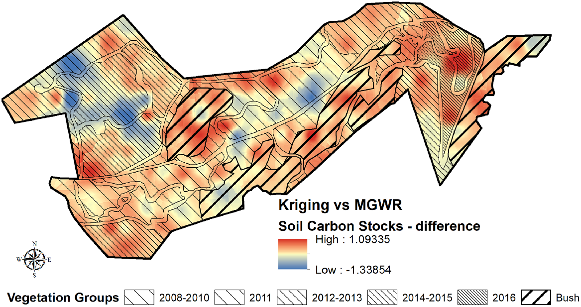
In order to understand potential disparities in soil carbon stock values generated by the two selected methods, we have created a map illustrating the variations in soil carbon stock values stemming from distinct MGWR-derived predictions and kriging-based estimates (Fig. 7). In regions with fewer data points, there is a notable trend of larger negative differences, indicating that kriging tended to overestimate values while GWR underestimated them. Conversely, areas with higher bulk density exhibit a tendency toward larger positive differences, with GWR surpassing kriging estimates.
Conclusions
From the predicted spatial distribution of soil characteristics (0–10 cm) and the associations between these characteristics, vegetation, and topography, possible influences were identified. The distribution of soil carbon stocks was driven mainly by topographic features, primarily elevation and slope. The mapping of these relationships between soil characteristics, topography, and vegetation, generated using ordinary kriging and MGWR, provided an innovative approach to examining these relationships and potential influences. The outcome of this study highlights the importance of taking landscape characterises into account when planning a forest restoration project.
Data availability
The data that support the findings of this study will be made available via Figshare.
Acknowledgements
The authors thank Mahrukh and Thomas Stazyk for graciously allowing us to carry out this research at CUE Haven, David Wackrow and Natalia Abrego for their technical expertise and support with the laboratory. We also acknowledge the students from the University of Auckland (Christopher Turner, Sophie Bialostocki, Madeline Daly, Lenna Kunisawa, Hannah Miller, Khendra Harvey, Alex McDonald and Emily Wexler) who helped with the fieldwork.
References
Adhikari K, Hartemink AE (2016) Linking soils to ecosystem services – a global review. Geoderma 262, 101-111.
| Crossref | Google Scholar |
Adhikari K, Mishra U, Owens PR, Libohova Z, Wills SA, Riley WJ, Hoffman FM, Smith DR (2020) Importance and strength of environmental controllers of soil organic carbon changes with scale. Geoderma 375, 114472.
| Crossref | Google Scholar |
Baldocchi D, Penuelas J (2019) The physics and ecology of mining carbon dioxide from the atmosphere by ecosystems. Global Change Biology 25, 1191-1197.
| Crossref | Google Scholar |
Ballance PF, McCarthy JA (1975) Geology of Okahukura peninsula, Kaipara Harbour, New Zealand. New Zealand Journal of Geology and Geophysics 18, 721-743.
| Crossref | Google Scholar |
Barrena-González J, Gabourel-Landaverde VA, Mora J, Contador JFL, Fernández MP (2023) Exploring soil property spatial patterns in a small grazed catchment using machine learning. Earth Science Informatics 16, 3811-3838.
| Crossref | Google Scholar |
Beever J (1981) A map of the pre-European vegetation of lower Northland, New Zealand. New Zealand Journal of Botany 19, 105-110.
| Crossref | Google Scholar |
Benayas JMR, Newton AC, Diaz A, Bullock JM (2009) Enhancement of biodiversity and ecosystem services by ecological restoration: a meta-analysis. Science 325, 1121-1124.
| Crossref | Google Scholar |
Berhe AA, Harte J, Harden JW, Torn MS (2007) The significance of the erosion-induced terrestrial carbon sink. BioScience 57, 337-346.
| Crossref | Google Scholar |
Carswell FE, Burrows LE, Hall GM, Mason NW, Allen RB (2012) Carbon and plant diversity gain during 200 years of woody succession in lowland New Zealand. New Zealand Journal of Ecology 36(2), 191-202.
| Google Scholar |
Chatterjee A, Lal R, Wielopolski L, Martin MZ, Ebinger MH (2009) Evaluation of different soil carbon determination methods. Critical Reviews in Plant Sciences 28, 164-178.
| Crossref | Google Scholar |
Chazdon R, Brancalion P (2019) Restoring forests as a means to many ends. Science 365, 24-25.
| Crossref | Google Scholar |
Contosta AR, Lerman SB, Xiao J, Varner RK (2020) Biogeochemical and socioeconomic drivers of above- and below-ground carbon stocks in urban residential yards of a small city. Landscape and Urban Planning 196, 103724.
| Crossref | Google Scholar |
Costa EM, Tassinari WdS, Pinheiro HSK, Beutler SJ, dos Anjos LHC (2018) Mapping soil organic carbon and organic matter fractions by geographically weighted regression. Journal of Environmental Quality 47(4), 718-725.
| Crossref | Google Scholar | PubMed |
Fotheringham AS, Charlton ME, Brunsdon C (1998) Geographically weighted regression: a natural evolution of the expansion method for spatial data analysis. Environment and Planning A: Economy and Space 30, 1905-1927.
| Crossref | Google Scholar |
Fotheringham AS, Yang W, Kang W (2017) Multiscale geographically weighted regression (MGWR). Annals of the American Association of Geographers 107, 1247-1265.
| Crossref | Google Scholar |
Gao L, Huang M, Zhang W, Qiao L, Wang G, Zhang X (2021) Comparative study on spatial digital mapping methods of soil nutrients based on different geospatial technologies. Sustainability 13(6), 3270.
| Crossref | Google Scholar |
Gregorich EG, Greer KJ, Anderson DW, Liang BC (1998) Carbon distribution and losses: erosion and deposition effects. Soil and Tillage Research 47, 291-302.
| Crossref | Google Scholar |
Griffiths RP, Madritch MD, Swanson AK (2009) The effects of topography on forest soil characteristics in the Oregon Cascade Mountains (USA): implications for the effects of climate change on soil properties. Forest Ecology and Management 257, 1-7.
| Crossref | Google Scholar |
Guo LB, Gifford RM (2002) Soil carbon stocks and land use change: a meta analysis. Global Change Biology 8, 345-360.
| Crossref | Google Scholar |
Guo LB, Wang M, Gifford RM (2007) The change of soil carbon stocks and fine root dynamics after land use change from a native pasture to a pine plantation. Plant and Soil 299, 251-262.
| Crossref | Google Scholar |
Harper AB, Powell T, Cox PM, et al. (2018) Land-use emissions play a critical role in land-based mitigation for Paris climate targets. Nature Communications 9, 2938.
| Crossref | Google Scholar |
Hedley CB, Lambie SM, Dando JL (2013) Edaphic and environmental controls of soil respiration and related soil processes under two contrasting manuka and kanuka shrubland stands in North Island, New Zealand. Soil Research 51, 390-405.
| Crossref | Google Scholar |
Henneron L, Balesdent J, Alvarez G, et al. (2022) Bioenergetic control of soil carbon dynamics across depth. Nature Communication 13, 7676.
| Crossref | Google Scholar |
Himestra P, Skoin JO (2023) automap: automatic interpolation package. Available at https://cran.r-project.org/web/packages/automap
Hong S, Yin G, Piao S, Dybzinski R, Cong N, Li X, Wang K, Peñuelas J, Zeng H, Chen A (2020) Divergent responses of soil organic carbon to afforestation. Nature Sustainability 3, 694-700.
| Crossref | Google Scholar |
Jensen JL, Christensen BT, Schjønning P, Watts CW, Munkholm LJ (2018) Converting loss-on-ignition to organic carbon content in arable topsoil: pitfalls and proposed procedure. European Journal of Soil Science 69(4), 604-612.
| Crossref | Google Scholar |
Kirschbaum MUF, Saggar S, Tate KR, Thakur KP, Giltrap DL (2013) Quantifying the climate-change consequences of shifting land use between forest and agriculture. Science of The Total Environment 465, 314-324.
| Crossref | Google Scholar |
Kruskal WH, Wallis WA (1952) Use of ranks in one-criterion variance analysis. Journal of the American Statistical Association 47, 583-621.
| Crossref | Google Scholar |
Kumar S, Lal R, Liu D, Rafiq R (2013) Estimating the spatial distribution of organic carbon density for the soils of Ohio, USA. Journal of Geographical Sciences 23, 280-296.
| Crossref | Google Scholar |
Kuśmierz S, Skowrońska M, Tkaczyk P, Lipiński W, Mielniczuk J (2023) Soil organic carbon and mineral nitrogen contents in soils as affected by their pH, texture and fertilization. Agronomy 13, 267.
| Crossref | Google Scholar |
Lark RM, Marchant BP (2018) How should a spatial-coverage sample design for a geostatistical soil survey be supplemented to support estimation of spatial covariance parameters? Geoderma 319, 89-99.
| Crossref | Google Scholar |
Lawrence CR, Harden JW, Xu X, Schulz MS, Trumbore SE (2015) Long-term controls on soil organic carbon with depth and time: a case study from the Cowlitz River Chronosequence, WA USA. Geoderma 247-248, 73-87.
| Crossref | Google Scholar |
Li J, Heap AD (2011) A review of comparative studies of spatial interpolation methods in environmental sciences: performance and impact factors. Ecological Informatics 6, 228-241.
| Crossref | Google Scholar |
Li J, Heap AD (2014) Spatial interpolation methods applied in the environmental sciences: a review. Environmental Modelling & Software 53, 173-189.
| Crossref | Google Scholar |
Lin S, Zhu Q, Liao K, Lai X, Guo C (2024) Mapping surface soil organic carbon density by combining different soil sampling data sources and prediction models in Yangtze River Delta, China. Catena 235, 107656.
| Crossref | Google Scholar |
LINZ (2023a) NZ 8m Digital Elevation Model (2012), Land Information New Zealand. Available at https://data.linz.govt.nz/layer/51768-nz-8m-digital-elevation-model-2012/
LINZ (2023b) NZ River Centrelines (Topo, 1:250k), Land Information New Zealand. Available at https://data.linz.govt.nz/layer/50182-nz-river-centrelines-topo-1250k/
Lozano-García B, Parras-Alcántara L, Brevik EC (2019) Impact of topographic aspect and vegetation (native and reforested areas) on soil organic carbon and nitrogen budgets in Mediterranean natural areas. Science of The Total Environment 544, 963-970.
| Crossref | Google Scholar |
Malik AA, Puissant J, Buckeridge KM, et al. (2018) Land use driven change in soil pH affects microbial carbon cycling processes. Nature Communications 9, 3591.
| Crossref | Google Scholar |
Martin DM (2017) Ecological restoration should be redefined for the twenty-first century. Restoration Ecology 25, 668-673.
| Crossref | Google Scholar | PubMed |
Mason NWH, Beets PN, Payton I, Burrows L, Holdaway RJ, Carswell FE (2014) Individual-based allometric equations accurately measure carbon storage and sequestration in shrublands. Forests 5(2), 309-324.
| Crossref | Google Scholar |
Messier C, Bauhus J, Sousa-Silva R, Auge H, Baeten L, Barsoum N, et al. (2021) For the sake of resilience and multifunctionality, let’s diversify planted forests!. Conservation Letters 15, e12829.
| Crossref | Google Scholar |
Mirchooli F, Kiani-Harchegani M, Darvishan AK, Falahatkar S, Sadeghi SH (2020) Spatial distribution dependency of soil organic carbon content to important environmental variables. Ecological Indicators 116, 106473.
| Crossref | Google Scholar |
Mitchell K (2010) Quantitative analysis by the point-centered quarter method. arXiv preprint arXiv:1010.3303.
| Google Scholar |
Mori AS (2017) Biodiversity and ecosystem services in forests: management and restoration founded on ecological theory. Journal of Applied Ecology 54, 7-11.
| Crossref | Google Scholar |
Morton JD, Baird DB, Manning MJ (2000) A soil sampling protocol to minimise the spatial variability in soil test values in New Zealand hill country. New Zealand Journal of Agricultural Research 43, 367-375.
| Crossref | Google Scholar |
Na M, Sun X, Zhang Y, Sun Z, Rousk J (2021) Higher stand densities can promote soil carbon storage after conversion of temperate mixed natural forests to larch plantations. European Journal of Forest Research 140, 373-386.
| Crossref | Google Scholar |
Oshan TM, Li Z, Kang W, Wolf LJ, Fotheringham AS (2019) mgwr: a Python implementation of multiscale geographically weighted regression for investigating process spatial heterogeneity and scale. ISPRS International Journal of Geo-Information 8, 269.
| Crossref | Google Scholar |
Pebesma E, Graeler B (2023) Gstat: spatial and spatio-temporal geostatistical modelling, prediction and simulation. Available at https://cran.r-project.org/web/packages/gstat/index.html
R Core Team (2021) ‘R: a language and environment for statistical computing.’ (R Foundation for Statistical Computing: Vienna, Austria) Available at https://www.R-project.org/
Saeed S, Sun Y, Beckline M, Chen L, Lai Z, Mannan A, et al. (2019) Altitudinal gradients and forest edge effect on soil organic carbon in Chinese fir (Cunninghamia lanceolata): a study from southeastern China. Applied Ecology & Environmental Research 17(1), 745-757.
| Google Scholar |
Schwendenmann L, Mitchell ND (2014) Carbon accumulation by native trees and soils in an urban park, Auckland. New Zealand Journal of Ecology 38(2), 213-220.
| Google Scholar |
Scott NA, Tate KR, Ford-Robertson J, Giltrap DJ, Smith CT (1999) Soil carbon storage in plantation forests and pastures: land-use change implications. Tellus B: Chemical and Physical Meteorology 51, 326-335.
| Crossref | Google Scholar |
Shapiro SS, Wilk MB (1965) An analysis of variance test for normality (complete samples). Biometrika 52, 591-611.
| Crossref | Google Scholar |
Song X-D, Yang F, Ju B, Li D-C, Zhao Y-G, Yang J-L, Zhang G-L (2018) The influence of the conversion of grassland to cropland on changes in soil organic carbon and total nitrogen stocks in the Songnen Plain of Northeast China. Catena 171, 588-601.
| Crossref | Google Scholar |
Sparling G, Schipper L (2004) Soil quality monitoring in New Zealand: trends and issues arising from a broad-scale survey. Agriculture, Ecosystems & Environment 104, 545-552.
| Crossref | Google Scholar |
Stockmann U, Adams MA, Crawford JW, Field DJ, Henakaarchchi N, Jenkins M, et al. (2013) The knowns, known unknowns and unknowns of sequestration of soil organic carbon. Agriculture, Ecosystems & Environment 164, 80-99.
| Crossref | Google Scholar |
Stutter MI, Lumsdon DG, Billett MF, Low D, Deeks LK (2009) Spatial variability in properties affecting organic horizon carbon storage in upland soils. Soil Science Society of America Journal 73, 1724-1732.
| Crossref | Google Scholar |
Sulman BN, Harden J, He Y, Treat C, Koven C, Mishra U, O’Donnell JA, Nave LE (2020) Land use and land cover affect the depth distribution of soil carbon: insights from a large database of soil profiles. Frontiers in Environmental Science 8, 146.
| Crossref | Google Scholar |
Trotter C, Tate K, Scott N, Townsend J, Wilde H, Lambie S, et al. (2005) Afforestation/reforestation of New Zealand marginal pasture lands by indigenous shrublands: the potential for Kyoto forest sinks. Annals of Forest Science 62, 865-871.
| Crossref | Google Scholar |
Volfová A, Šmejkal M (2012) Geostatistical methods in R. Geoinformatics FCE CTU 8, 29-54.
| Crossref | Google Scholar |
Wang K, Zhang C, Li W (2012) Comparison of geographically weighted regression and regression kriging for estimating the spatial distribution of soil organic matter. GIScience & Remote Sensing 49, 915-932.
| Crossref | Google Scholar |
Wiesmeier M, Urbanski L, Hobley E, Lang B, von Lützow M, Marin-Spiotta E, et al. (2019) Soil organic carbon storage as a key function of soils – a review of drivers and indicators at various scales. Geoderma 333, 149-162.
| Crossref | Google Scholar |
Zhang Z, Zhou Y, Huang X (2020) Applicability of GIS-based spatial interpolation and simulation for estimating the soil organic carbon storage in karst regions. Global Ecology and Conservation 21, e00849.
| Crossref | Google Scholar |
Zhong H, Smith C, Robinson B, Kim Y-N, Dickinson N (2017) Plant litter variability and soil N mobility. Soil Research 55(3), 253-263.
| Crossref | Google Scholar |
Zhu C, Wei Y, Zhu F, Lu W, Fang Z, Li Z, Pan J (2022) Digital mapping of soil organic carbon based on machine learning and regression kriging. Sensors 22, 8997.
| Crossref | Google Scholar |