
Seasonal climate summary for the southern hemisphere (autumn 2018): a weak La Niña fades, the austral autumn remains warmer and drier
Bernard Chapman A B and Katie Rosemond A BA Bureau of Meteorology, GPO Box 413, Brisbane, Qld 4001, Australia.
B Corresponding authors. Email: bernard.chapman@bom.gov.au; katie.rosemond@bom.gov.au
Journal of Southern Hemisphere Earth Systems Science 70(1) 328-352 https://doi.org/10.1071/ES19039
Submitted: 18 February 2020 Accepted: 22 May 2020 Published: 19 November 2020
Journal Compilation © BoM 2020 Open Access CC BY-NC-ND
Abstract
This is a summary of the austral autumn 2018 atmospheric circulation patterns and meteorological indices for the southern hemisphere, including an exploration of the season’s rainfall and temperature for the Australian region. The weak La Niña event during summer 2017–18 was in retreat as the southern hemisphere welcomed the austral autumn, and before midseason, it had faded. With the El Niño Southern Oscillation and the Indian Ocean Dipole in neutral phases, their influence on the climate was weakened. Warmer than average sea surface temperatures dominated much of the subtropical South Pacific Ocean and provided favourable conditions for the formation of a rare subtropical cyclone over the southeast Pacific Ocean in May. The southern hemisphere sea ice extent was slightly below the autumn seasonal average. The southern hemisphere overall during autumn was drier and warmer than the seasonal average. The season brought warmer than average temperatures and average rains to parts of the continents of Africa and South America. Australia recorded its fourth-warmest autumn, partly due to an intense, extensive and persistent heatwave, which occurred during the midseason. An extraordinary and record-breaking rainfall event occurred over Tasmania’s southeast, under the influence of a negative Southern Annular Mode. The mainland’s northeastern tropical region was wetter than average as a result of tropical cyclones, which formed during an active monsoon. These areas, however, were in contrast to the rest of the continent, which followed the trend of the previous season and remained drier than average; consequently, rainfall deficiencies emerged across the southern half of Australia, and some areas witnessed an increase in extent and severity of these deficiencies.
Keywords: 2018, Antarctic sea ice, autumn, climate summary, El Niño, ENSO, Indian Ocean Dipole, La Niña, Pacific, seasonal summary, southern hemisphere.
1 Introduction
This summary reviews the southern hemisphere and equatorial climate patterns for autumn 2018, with particular attention given to the Australasian and equatorial regions of the Pacific and Indian ocean basins. The main sources of information for this report were analyses prepared by the Australian Bureau of Meteorology, the United States National Oceanic and Atmospheric Administration (NOAA) and the Global Precipitation Climatology Centre (GPCC).
2 Pacific and Indian ocean basins climate indices
2.1 Southern Oscillation Index (SOI)
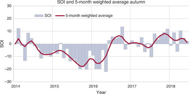
Sustained negative values of SOI below –7 are often indicative of El Niño episodes, while sustained positive values of SOI above +7 are typical of La Niña. The SOI sustained positive values during the 2017–18 summer, with a weak La Niña event occurring between December 2017 and January 2018. This La Niña episode began to weaken during January and February 2018, before ending in the first month of the austral autumn, and El Niño Southern Oscillation (ENSO) conditions returned to neutral territory. Data showed the SOI values remained below +7 during April and May, indicating the ENSO influence on the climate remained weak.
The monthly SOI value for March (+10.5) fell during April and May, with monthly values of +4.5 and +2.1, respectively. The autumn 2018 mean value of the SOI was +5.7.
The Troup SOI1 for January 2014 to May 2018 is shown in Fig. 1, along with a five-month weighted, moving average of the monthly SOI.
|
The autumn average mean sea level pressure (MSLP) value for Darwin was 0.2 hPa below average at 1009.3 hPa and 0.8 hPa above average for Tahiti with 1012.8 hPa. The monthly anomalies for Darwin in March, April and May 2018 were –1.7, –0.1 and +1.1, respectively, and for Tahiti, +0.5, +0.7 and +1.4, respectively. The overall negative anomaly at Darwin was consistent with a wetter than average autumn for the region.
2.2 Composite monthly ENSO Index (5VAR)
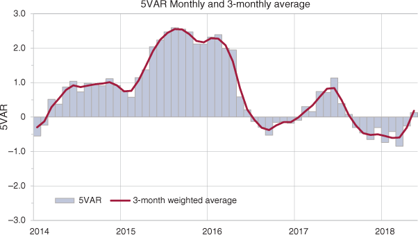
The ENSO 5VAR Index2 is a composite monthly ENSO index calculated as the standardised amplitude of the first principal component of the monthly Darwin and Tahiti MSLP and monthly indices NINO3, NINO3.4 and NINO4 sea surface temperatures (SSTs)3. Values of the 5VAR that are in excess of one standard deviation are typically associated with El Niño for positive values, while negative 5VAR values of a similar magnitude are indicative of La Niña.
The 5VAR Index fell below +1 from July 2017 (Fig. 2), which is consistent with a neutral ENSO (Tobin 2020) and the onset of a weak La Niña in the latter stages of 2017 (Tihema 2019). NINO3.4 values were below zero from July 2016 until early 2017 (Trewin 2018a). The index went slightly positive from March 2017 and remained at this level until September before dipping into negative territory and reaching its lowest value of around –0.8°C late in 2017.
|
The negative values late in 2017 persisted into autumn 2018, with slightly negative values of the 5VAR Index for March (−0.85) and April (−0.26), falling short of the La Niña thresholds. The 5VAR moved into slightly positive territory by the end of May (+0.13).
2.3 Indian Ocean Dipole (IOD)
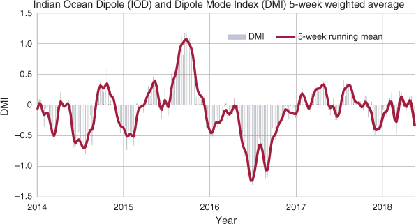
The IOD4 (Saji et al. 1999) exhibits three phases that are defined by the sign and magnitude of the difference between the equatorial Indian Ocean temperatures of the western node (in the waters off the coast of Somalia) and the eastern node (in waters off the coast of Sumatra). The IOD is said to be in a positive phase when values of the Dipole Mode Index (DMI) are greater than 0.4°C. When the DMI is sustained between –0.4°C and 0.4°C, the IOD is neutral. When the DMI values are less than –0.4°C, the IOD is in a negative phase.
During the months of December–April, phases of the IOD are generally less influential due to the southward movement of the monsoon, which changes the atmospheric circulation. However, the influence of the IOD may manifest between April and November when the monsoon typically contracts northward. A strongly positive IOD developing in middle–late autumn is characterised by the lack of warm maritime airflow from west to east. In this phase, continental Australia has an increased chance of a drier than average winter. If the positive IOD is sustained or strengthens then there is an elevated chance of less than average spring rainfall.
The IOD (Fig. 3) was in a weakly negative phase during March 2018, with DMI values reaching the season’s strongest negative value of –0.47°C. The IOD then retreated into a neutral phase at the start of April. By midseason, values of DMI were in the neutral range (+0.06°C), and after just a brief and shallow dip to –0.09°C, the DMI continued to move towards positive values. The neutral phase that had dominated throughout the season continued to the end with negative values still in the neutral range in May, ending with –0.33°C. The IOD was firmly in a neutral phase when autumn gave way to winter.
|
Studies of impacts on the Australian region during both coincident negative IOD and La Niña phases, and coincident positive IOD and El Niño phases, have shown that the combined effects of both phases are enhanced. These climate drivers heighten impacts regarding rainfall and temperature. While it is recognised that there is a relationship between the two drivers, the relationship is complex, and as such, it continues to be an active area of research (Santoso et al. 2019).
3 Outgoing longwave radiation (OLR)
OLR in the equatorial Pacific Ocean can be used as an indicator of enhanced or suppressed tropical convection. Increased positive OLR anomalies typify a regime of reduced convective activity, a reduction in cloudiness and, usually, a reduction in rainfall. Conversely, negative OLR anomalies indicate enhanced convection, increased cloud-cover and chances of increased rainfall. During La Niña, decreased convection (increased OLR) can be seen near the Date Line, whereas increased cloudiness (decreased OLR) near the Date Line usually occurs during El Niño. When Australia is under the influence of a positive IOD event, OLR anomalies are positive over the eastern Indian Ocean where convective activity is typically reduced.
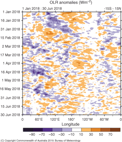
The Hovmöller diagram of OLR anomalies along the equator during January–June 2018 (Fig. 4) shows that convection was generally suppressed over the central to eastern equatorial Pacific and enhanced across Indonesia and the western equatorial Pacific during January–March. Collectively, these oceanic and atmospheric anomalies reflected weak La Niña conditions. ENSO-neutral conditions were mirrored in the slight changes in convection, remaining suppressed over the central and eastern equatorial Pacific and slightly enhanced over the western equatorial Pacific and the Indonesia region during April–May.
|
Averaged over an area at the International Date Line (7.5°S–7.5°N and 160°E–160°W), the standardised monthly OLR anomaly was +0.5 for March, +1.2 for April and +1.0 for May. The autumn 2018 average was +0.9.
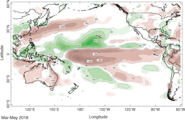
Seasonal spatial patterns of OLR anomalies across the Asia–Pacific region between 40°S and 40°N for the southern hemisphere autumn 2018 are shown in Fig. 5. Negative OLR anomalies were evident across the Maritime Continent and western Pacific with the strongest anomalies discernible over the Solomon Islands and parts of eastern Indonesia. The persistence of the near equatorial trough, which helped focus convection in these areas, was one of the main instigators of these anomalies through the second half of April and into May. The South Pacific convergence zone become a more persistent feature during the second half of April and during May. The lowest negative anomaly (of –20.7 Wm−2) featured in autumn 2018 over the southern Solomon Islands. An area of negative anomalies in the range 5–25 Wm−2 around Sumatra and extending westwards to southern India possibly indicated initial development of a positive IOD. The strongly positive OLR anomalies off northwest Australia and Java indicated less moisture than normal in the atmosphere, typical of a positive IOD phase. Typically, it is in autumn or winter when either a negative, or positive IOD phase emerges.

|
Tropical cyclone activity in the second half of March likely contributed to the slightly negative anomalies around the Gulf of Carpentaria. Further tropical cyclone activity in the southwest Pacific during the early part of April was also reflected in the negative anomalies detected around the eastern Coral Sea.
The dominance of the trade flow pattern kept clouds suppressed, especially over continental Australia. Accordingly, the anomalies were generally insignificant, although parts of southeastern and southern Australia recorded anomalies in excess of 5 Wm−2 above the seasonal mean.
However, there were suspected negative biases in the OLR anomalies over subtropical land areas where they are estimated to be around 5 Wm−2, the bias is due to satellite orbit decay (M. Wheeler, pers. comm. October 2019). A map is provided of the seasonal precipitation anomalies (Fig. 6) as calculated from NOAA’s Climate Anomaly Monitoring System-OLR Precipitation Index (CAMS_OPI) analysis for the Pacific region.
|
4 Madden-Julian Oscillation (MJO)
The MJO5 is a tropical convective wave anomaly, which develops in the Indian Ocean and propagates eastwards into the Pacific Ocean (Madden and Julian 1971, 1972, 1994). The MJO takes approximately 30–60 days to reach the western Pacific, with a frequency of six–twelve events per year (Donald et al. 2004). When the MJO is in an active phase, it is associated with areas of increased and decreased tropical convection, with effects on the southern hemisphere often weakening during early autumn, before transitioning to the northern hemisphere. A description of the Real-time Multivariate (RMM) MJO index and the associated phases can be found in Wheeler and Hendon (2004).
The phase-space diagram of the RMM for autumn 2018 is shown in Fig. 7. In the first week of March, the MJO was in phase 2 and close to phase 3 over the Indian Ocean with modest strength. It then embarked on a weakening trend as it tracked further east within the second week of March, returning to the unit circle before entering phase 4 and 5, over the Maritime Continent, during the second half of March. The impact of a Kelvin wave, which temporarily complicated the MJO signal by weakening it and initially retrogressing it towards phase 2 is shown in Fig. 6. After some stalling of the oscillation, it resumed moving into phase 4 and 5 over the Maritime Continent with modest strength.
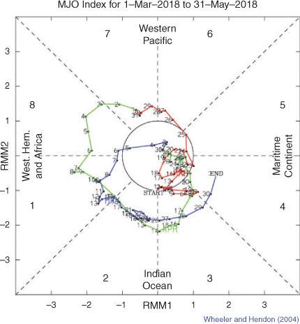
|
Analysis indicated the MJO was still in phase 3 over the Indian Ocean in the first week of March, but the signal had become incoherent with significant weakening. However, a strong equatorial Rossby wave moving through Australian longitudes enhanced convection in the area and was likely responsible for the development of tropical cyclones Hola, Linda and Marcus during the first half of March and tropical cyclones Nora and Iris towards the last week of March. The MJO progressed from phases 4 and 5 into phases 6 and 7 over the western Pacific Ocean in late March and early April, where it emerged as a stronger signal.
Tropical cyclone Josie briefly formed in response to the strengthened MJO signal in late March and very early April. The MJO signal maintained moderate strength as it progressed eastwards from phase 7, over the western Pacific, into phase 8 over the western hemisphere and Africa, during the first week and a half of April. Tropical cyclone Keni formed to the east of Vanuatu during this time because of cross-equatorial flow into a near-stationary convergence zone from the Solomon Islands to Fiji. The MJO signal continued its eastward progression and eventually weakened to be within the unit circle in the last 10 days of April. The last week of April saw a double near equatorial trough structure, a common feature of the transition from the southern hemisphere tropical cyclone season to the northern hemisphere tropical cyclone season. The MJO remained weak and indiscernible inside the unit circle, having little influence on tropical weather. The phase diagram showed the MJO remained in a similar state into the first week of May.
The westwards propagating Rossby wave caused a flaring of convection, and its persistence and organisation led to the development of tropical cyclone Flamboyan over the far northern Indian Ocean in the last days of April.
The moderate pulse of the MJO (at the edge of phase 1 moving into phase 2) also assisted in the formation of two significant tropical systems in middle–late May. Tropical cyclone Sagar was spawned near the Horn of Africa around 17 May, while tropical cyclone Mekunu formed near the Arabian Peninsula on 23 May before it made landfall over southern Oman late on the 25 May. The system delivered heavy rainfall, flash flooding and damaging surf conditions as it crossed the coast near Salalah. Impacts were also substantial on the Socotra Islands, Yemen.
5 Oceanic patterns
5.1 Sea surface temperatures (SSTs)
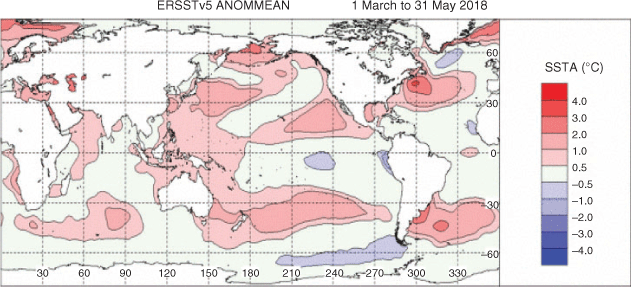
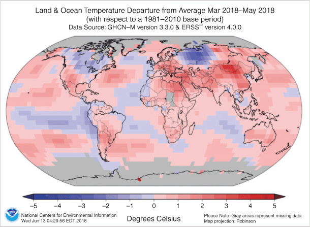
The SST anomaly for the combined ocean area of the southern hemisphere for autumn 20186 was +0.57°C above the 20th century seasonal average. This was the eighth-warmest value on record in the NOAA data set for austral autumns 1901–2019. Though warmer than autumn 2017, it was cooler (−0.21°C) than the record warm SSTs experienced during the austral autumn of 2016 (+0.78°C) (Rosemond and Tobin 2018). The global SST anomalies for autumn 2018, relative to 1961–2000, are shown in Fig. 8.
|
During autumn 2018, the tropical Pacific returned to ENSO-neutral, as indicated by mostly near to below SSTs over the east-central equatorial Pacific and below average SSTs near the west coast of South America (Fig. 8). Warm anomalies were present across most of the South Pacific around and to the south of 30°S. Warm anomalies were also widespread over the Maritime Continent. The monthly El Niño indices were near zero to slightly below average, except for NINO1 +2, which remained negative (at –1.0°C). Subsurface temperature anomalies (averaged across 180°–100°W) remained positive, due to the continued influence of a downwelling oceanic Kelvin wave. Atmospheric indicators related to last season’s La Niña also continued to fade.
The NINO3.4 index, which measures SSTs in the central Pacific Ocean between 5°N–5°S and 120°–170°W, is used by the Australian Bureau of Meteorology to monitor ENSO; NINO3.4 is closely related to the Australian climate (Wang and Hendon 2007).
7The NINO3 monthly temperature anomalies were –0.6°C, –0.2°C and 0.0°C for March, April and May, respectively, although the monthly temperature anomalies for NINO3.4 were similar, being –0.6°C, –0.3°C and 0.0°C. The NINO4 monthly anomalies were only marginally above the monthly anomalies for each month of the austral autumn 2018, March (0.0°C), April (0.1°C) and May (0.2°C).
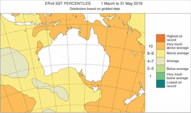
The SSTs in the Australian region (Fig. 9), based on Extended Reconstructed Sea Surface Temperature version 5 (ERSSTv5) data, were at least 0.5°C above the seasonal average over the Tasman and Coral seas, as well as the Indian Ocean off the western coastline of Australia, the Timor and Arafura Sea and the Gulf of Carpentaria around the northern coastline. Anomalies of 1–2°C were widespread across the Tasman Sea after the exceptionally warm SSTs occurred from the second half of November until early 2018. The SSTs in these regions were much warmer than any SSTs previously recorded at that time. This area extended west from New Zealand to Tasmania and in waters surrounding mainland southeast Australia.8
|
5.2 Subsurface ocean temperatures
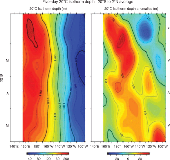
The 20°C isotherm depth is generally located close to the equatorial thermocline, which is the region of greatest temperature gradient with depth and the boundary between the warm near-surface and cold deep-ocean waters. Therefore, measurements of the 20°C isotherm depth make a good proxy for the thermocline depth. Negative anomalies correspond to the 20°C isotherm being shallower than average and are indicative of cooling of subsurface temperatures. If the thermocline anomaly is positive, the thermocline is deeper. A deeper thermocline results in less cold water available for upwelling, and therefore, a warming of subsurface temperatures.
The four-month sequence of subsurface temperature anomalies (Fig. 10) shows the decay of shallow cool anomalies in the eastern equatorial Pacific Ocean during February–May 2018. There was an eastward propagation of warmer than average water further below the surface. The area of warm anomalies extended from 140°E to 120°W between 100–200 m depth.
|
This is typical during the breakdown of La Niña, which acts to dilute the cool subsurface waters in the eastern Pacific as the warmer than average subsurface water propagates eastwards. In Fig. 10, a pool of warmer than average water between 140°E and 140°W in a depth between 120–200 m with cool anomalies in the shallow subsurface of the eastern equatorial Pacific Ocean, is shown. Towards mid and late May, a pool of warmer than average water tracked eastwards and affected SSTs as these warmer waters shoaled in the eastern Pacific.
Subsurface water with generally positive temperature anomalies (averaged across 180°–100°W) increased from April to May, as another downwelling equatorial oceanic Kelvin wave reinforced the already above average subsurface temperatures (Fig. 11).

|
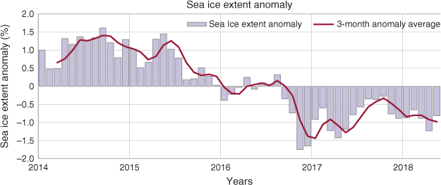
6 Sea ice
Autumn 2018 continued a recent trend with Antarctic sea ice extents contracting well below the 1981–2010 seasonal average and below even the long-term range of variability for nearly every month. Extents for 2017 and 2018 were the lowest on record for both winter maximum and summer minimum.9 During autumn 2018, the Antarctic sea ice extent was slightly below the 1981–2010 average throughout the season. Sea ice extents were below the long-term average for March, April and May by 12.4, 12.3 and 8.6% over the three months, respectively. Sea ice extent was approximately 520 000 km2 less than the 1981–2010 average and ranked as the seventh lowest sea ice extent on record for March. April also saw a sea ice extent that was approximately 830 000 km2 below the April average. The total sea ice extent in May was 9 300 000 km2; and this was 855 000 km2 less than the monthly average. It was the third lowest sea ice extent on record. Its northward extent was less than average for May in all sectors, particularly in the eastern Weddell Sea and the Ross Sea. There were above average areas of sea ice extent, but it was minimal and occurred in an area slightly eastward of the Shackleton Ice Shelf and over parts of the Amundsen Sea.10 A period of record to near-record high seasonal sea ice extents as depicted in Fig. 12, ended in the southern hemisphere winter prior to 2015 (Trewin 2018a).
|
7 Atmospheric circulation
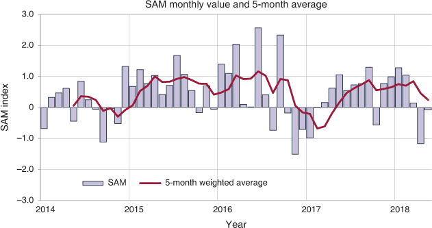
7.1 Southern Annular Mode (SAM)
The strength and position of cold fronts and midlatitude low pressure systems are important drivers of rainfall variability across southern Australia. In a positive SAM event, the belt of strong westerly winds contracts towards Antarctica. This results in weaker than normal westerly winds and higher pressures over southern Australia, restricting the penetration of cold fronts inland. During autumn and winter, a positive SAM value11 can mean cold fronts and lows farther south than average, and hence, the southern parts of Australia can experience low rainfall during these seasons (Hendon et al. 2007).
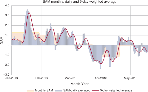
There was a strongly positive SAM phase during the early part of autumn 2018 (Fig. 13) with index values above +1 to 27 March. A transition to a negative phase occurred thereafter, and the SAM remained strongly negative for the majority of the next 30 days to 27 April. Positive SAM values returned from 28 April, and the SAM remained in this phase until about the middle of May. Some fluctuations occurred late in the season, though for the majority of the second half of May, indices were negative. Monthly mean values of the Climate Prediction Center (CPC) SAM index were +0.14 for March, –1.17 for April and –0.08 for May. The effect that the SAM can have on rainfall varies greatly depending on season and region, and despite the strongly negative mean value for April, rainfall was mostly below average across southern Western Australia, southern Victoria and Tasmania. Above to very much above average rainfall occurred over southern Victoria and parts of western and southern Tasmania in May.
|
With a negative phase of the SAM through the first half of April (Fig. 14), cold fronts produced strong to gale force winds, brought thunderstorms and extensive areas of raised dust on 13–14 April. The fronts also generated damaging winds across Victoria, including the state’s strongest gust of 128 km h−1 at the Wilsons Promontory lighthouse on 15 April. The strong winds and associated low pressure system linked to the fronts also contributed to high storm tides along parts of the Victorian coastline. In Tasmania, strong and gusty winds were common from 13 to 16 April, also associated with a series of cold fronts. Winds were especially strong on the morning of 16 April, and many sites reported gusts in excess of 100 km h−1, peaking at 163 km h−1 at Maatsuyker Island. A vigorous cold front visited Tasmania, supported by the negative phase of the SAM and brought exceptionally high rainfall around mid-May.
|
7.2 Surface analyses
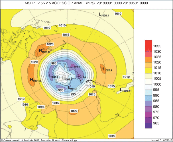
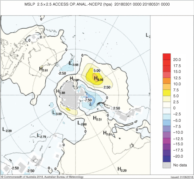
The average MSLP pattern for autumn 2018 is shown in Fig. 15, computed using data from the 0000 UTC daily analyses of the Bureau of Meteorology’s Australian Community Climate and Earth System Simulator (ACCESS) model.12 The MSLP anomalies relative to the 1979–2000 climatology shown in Fig. 16 were obtained from the National Center for Environmental Prediction (NCEP) reanalysis data (Kanamitsu et al. 2002). The MSLP anomaly field is not shown over areas of elevated topography (indicated by grey shading).
|
|
The analysis chart for the austral autumn 2018 depicted a pattern of relatively weak MSLP anomalies. However, there was a strong positive anomaly around 130°W where the subtropical ridge extended further south of the South Pacific Ocean. Slight positive anomalies were also evident over the far south of South America, where an anomalous ridge likely contributed to the below average autumn rainfall over Argentina. Similarly, for southern Australia, a slightly positive MSLP anomaly also delivered rainfall that was very much below the seasonal autumn average. Conversely, a strong negative anomaly in vicinity of the Antarctic Peninsula extending into the southeast Pacific Ocean (around 50–70°S, 80°W) depicted an anomalous trough (with MSLP anomalies of below –5 hPa). On 9 May 201813 an extremely rare subtropical cyclone was observed over the southeast Pacific Ocean (well off the coast of Chile). The MSLP anomaly was near slightly above average over most of Africa, South America and Australia but was below average over New Zealand.
7.3 Mid-tropospheric analyses
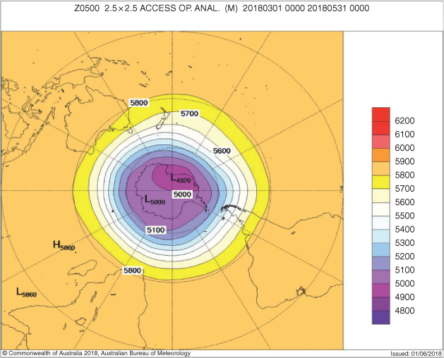
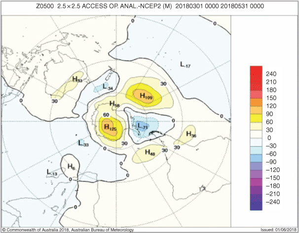
The average 500 hPa geopotential height for autumn 2018, shown in Fig. 17, is an indicator of the steering of surface synoptic systems across the southern hemisphere, it depicts a weak three-wave pattern with troughs located just west of the 180°W parallel, 90°W and approximately 30°E. The 500 hPa geopotential height anomaly map for autumn 2018 in Fig. 18 highlights the departure from the geopotential height seasonal average for autumn. The geopotential height is valuable when identifying upper level troughs, similar to a surface low pressure system, and the upper level ridging which is equivalent to surface high pressure systems.
|
|
The characteristic zonal structure of the middle to high latitudes is evident in the autumn 500 hPa anomaly pattern (Fig. 17), with weak three-wave characteristics evident. The mean 500 hPa circulation during March featured above average heights over the Indian Ocean and the central South Pacific with below average heights over the high latitudes of the eastern South Pacific. In April, there were above average heights over southeastern Australia, the high latitudes of the central South Pacific, southern South America and the western South Atlantic. The anomaly map (Fig. 18) featured below average heights over the western South Pacific and Indian Ocean. In southern South America and Australia, anomalous upper-level ridges contributed to exceptionally warm and dry conditions. Many locations recorded temperatures in the upper 90th percentile and the lowest 30th percentile for precipitation seasonally for autumn 2018.
8 Winds
Autumn 2018 low-level (850 hPa) and upper-level (200 hPa) wind anomalies shown in Figs 19 and 20 are from winds computed from ACCESS, and anomalies are computed with respect to the 22-year 1979–2000 NCEP climatology. Isotachs are at an interval of 5 ms−1.

|

|
The autumn 2018 wind anomalies at 850 hPa for the austral autumn (Fig. 19) were generally within 5 ms−1 of the long-term average. Mostly weak easterly low-level wind anomalies were evident across much of Australia, while a weak westerly anomaly dominated the far southeast of Australia and adjacent parts of the Tasman Sea. A discrete cyclonic circulation could be observed over the far southern Tasman Sea/Southern Ocean between Tasmania and New Zealand, this region corresponded with anomalies at the surface. An anticyclonic circulation in the far southern Pacific Ocean, around 40–50°S and 150–130°W was evident. Reduced cloud cover due to strong subsidence, promoted positive SST anomalies in the order of 1–2°C while vertical mixing between the upper and lower sections of the subsurface ocean was similarly limited.
At 200 hPa, autumn 2018, there were westerly anomalies (Fig. 19) present across much of the southern hemisphere in the 30–50°S latitude band. A trough in the easterly flow pattern dominated Australia. The central and eastern South Pacific saw a more involuted upper wind regime and anomalous westerly winds.
The circulation at 200 hPa across the subtropical Pacific Ocean in March in both hemispheres continued to reflect La Niña. The La Niña signal included amplified troughs east of the Date Line in the subtropics of both hemispheres in association with the disappearance of deep tropical convection from the central and eastern equatorial Pacific. The La Niña signal also included a focusing of the subtropical ridges over Australasia in association with enhanced convection over the western tropical Pacific and Indonesia. At 200 hPa, the subtropical circulation featured an amplified trough over the central and eastern South Pacific Ocean during April, which reflected lingering La Niña conditions.14
9 Australian region
9.1 Rainfall
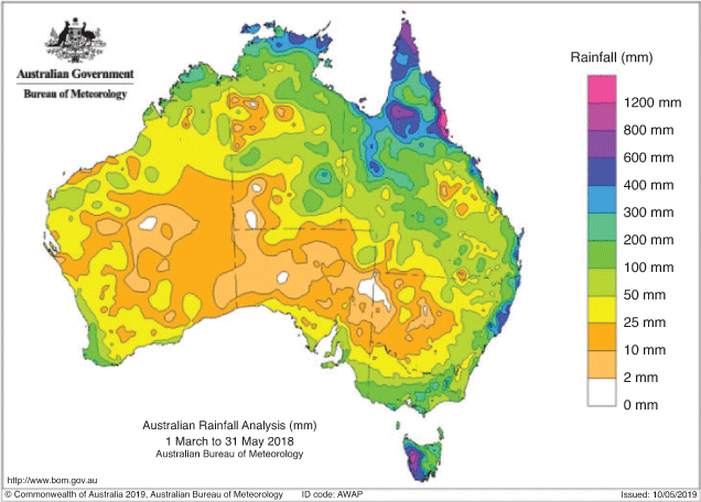
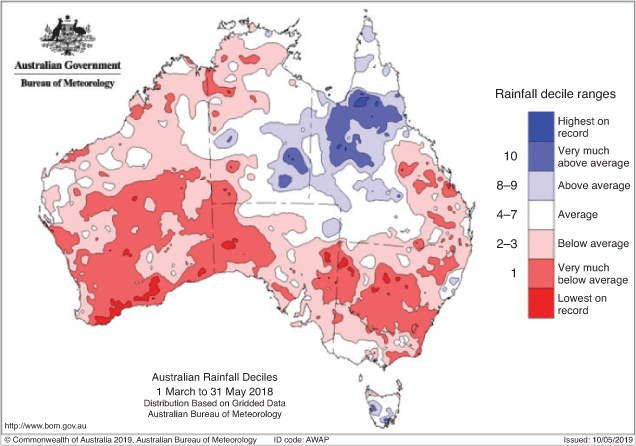
Overall, autumn 2018 was the second-driest autumn on record for Australia. It was 33.8% drier than the historical area-averaged seasonal mean rainfall of 79.7 mm (see Table 1). Notably, over Western Australia and New South Wales, large areas experienced very much drier than average conditions with sizable portions of each state recording totals that were in the lowest 10% of historical autumn rainfall totals (rainfall totals are shown in Fig. 21). The area-averaged rainfall was the lowest since 2005 for New South Wales and the state’s seventh-driest autumn on record. In Western Australia, it was the fourth-driest autumn since 1994. The area-averaged rainfall in South Australia was also very much below the seasonal mean, and it was also a drier than average autumn for Victoria and the Northern Territory.

|
|
Autumn was wetter than average for the Australian mainland’s northern tropics, eastern parts of the Northern Territory and much of Tasmania, with both Queensland and Tasmania recording positive rainfall anomalies for the season (Fig. 22). Above to very much above average rainfall occurred in much of the southern parts the Northern Territory as well as western, central and much of northern Queensland.
|
A broad area of low pressure over northern Australia during March provided conditions conducive to receiving above average rainfall. A low pressure centre deepened to the west of Townsville during the first week of March. The system brought heavy rainfall as it drifted to the west across the northern interior of Queensland. The low then tracked into the northwest interior and deepened, producing rainfall in excess of 100 mm. Another low, near the southern Gulf of Carpentaria and combined with low-level convergence on its eastern flank, caused several days of very heavy rainfall along the north tropical coast of Queensland around the middle of March, resulting in major riverine flooding. A rainband produced widespread, moderate to locally heavy rainfall, stretching from the Gulf Country, through inland Queensland to northeast New South Wales.
Rainfalls associated with tropical cyclones Marcus and Nora also weighed heavily on March rainfall totals across northern Queensland and far northern areas of the Northern Territory and Western Australia. Tropical cyclone Marcus produced extensive shower and thunderstorm activity with moderate to heavy falls across the Top End of the Northern Territory and north Kimberley in Western Australia in mid-March. The system went on to become the most intense tropical cyclone in the Australian region for more than a decade, reaching category five, on 21 and 22 March. During the last week of March, severe tropical cyclone Nora and its remnants, in association with the monsoon trough, generated moderate to heavy rainfall in far northern parts of the Northern Territory as well as very heavy rainfall and flooding in the Gulf Country and Cape York Peninsula. A large part of Queensland also experienced rainfall from this system, particularly northern and western parts of the state. Also, during the last week of March, a trough near the coast of southeast Queensland and New South Wales was cradled by a large, slow-moving high pressure system near Tasmania. This resulted in a very heavy rainfall event between Newcastle and Coffs Harbour, with rainfall totals that were in excess of 400 mm recorded in the seven-day period 20–27 March around the Mid North Coast of New South Wales.
A slightly negative SAM from mid-April translated to a more frequent period of westerly winds and embedded cold fronts, which affected Tasmania’s rainfall. An area of complex low pressure situated over eastern Bass Strait produced above average May rainfall for much of eastern Tasmania. Specifically, on 10 and 11 May, it brought record-breaking rain which led to major flooding on the catchments around the Wellington Range and Hobart. One record daily total was recorded at kunanyi (Mount Wellington), which observed a daily rainfall total of 236.2 mm on 11 May. Over 40% of Tasmania recorded rainfall above the highest May percentile on 11 May, and 24.9% of the state recorded their highest May daily rainfall since records began in the 24 hours to 9 a.m. on 11 May.
Five tropical cyclones occurred in the Australian region during autumn: Linda, Marcus, Nora, Iris and Flamboyan. Cyclones Linda and Iris were located off Australia’s eastern coast, but they did not make landfall, while Flamboyan remained well offshore and away from the continent’s western coast during its late April and early May lifespan.
Tropical cyclone Marcus15 was the strongest tropical cyclone to affect Darwin since severe tropical cyclone Tracy in December 1974. The system also became the strongest tropical cyclone anywhere within the Australian region since severe tropical cyclone Monica in April 2006. Dvorak analyses and other intensity estimation techniques indicated a similar direct comparison at peak intensity of both these tropical cyclones. Tropical cyclone Marcus formed about 300 km northeast of Darwin on 16 March. It was upgraded to a category two system and made landfall northeast of Darwin on 17 March. Marcus was a small system, but its impacts on Darwin were widespread and significant. Felled trees damaged buildings and cars, while downed powerlines caused significant power outages. Marcus made landfall on another two occasions: the first over the western Top End, and over the northern Kimberley. Marcus then moved out into the warm ocean waters off the north Kimberley coast. Here, Marcus rapidly intensified early on 19 March, and by late afternoon it had become a category three severe tropical cyclone. Severe tropical cyclone Marcus continued to intensify, reaching category five on 21 March. It adopted a consistent westerly track, away from the Western Australian coast, remaining at category five before it turned southward, and in doing so, eventually weakened below tropical cyclone intensity on 24 March, well offshore of the mid-coast of Western Australia.
Severe tropical cyclone Nora made landfall along the southwest Cape York Peninsula coast as a category three system late on 24 March. Several houses were damaged and numerous trees and power lines were brought down. Nora was also responsible for propagating large waves that pounded the western Cape York Peninsula coast, and north of the location where Nora made landfall, the storm surge reached 1.2 m at the Weipa tide gauge.16
Total rainfall for Australia’s Indian Ocean islands for March–May was close to average for the Christmas Island Aero and somewhat below average at the Cocos Island Airport. Subantarctic Macquarie Island saw well above average rainfall, and each month of autumn was wetter than average. Below average rainfall occurred at both Lord Howe and Norfolk islands.
9.2 Rainfall deficiencies
The isolated but reasonably intense periods of rainfall associated with the cyclones visiting Australia’s tropical north, as well as the extraordinary rainfall in Tasmania, did have some impact on deficiencies that were being tracked by the Bureau of Meteorology through the 2018 austral autumn.
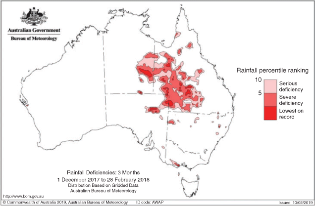
As the austral autumn arrived, it brought with it the deficiencies from the previous season, which is traditionally the wet season across northern Australia. For Queensland’s western and southern areas, the wet season had been dry, and deficiencies had emerged at the three-month time scale (Fig. 23). By the season’s end, Australia’s northern tropical region had experienced near-average areal autumn rainfall while the northeastern part of the continent was wetter than the northwest. In northeastern tropical regions, an active monsoon led to well above average rainfall and, in a smaller area, record high precipitation for March. This rainfall effectively removed the deficiency over the same region that had emerged over the last month of summer, at the three-month time scale.
|
Midseason rainfall was patchy over southern Australia. In southeastern Australia, the autumn areal average was 79.74 mm, the 12th-driest areal autumn rainfall on record for this part of the continent. Australia’s southwest received almost the equivalent areal averaged rainfall over autumn with 80.13 mm. This ranked as southwestern Australia’s seventh-driest autumn on record.
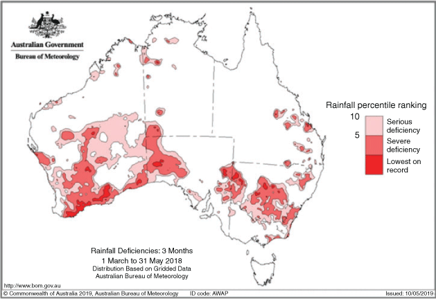
The lack of rainfall through late autumn for much of mainland Australia (Fig. 24) led to the emergence of serious to severe rainfall deficiencies across the southeast and the southwest. Conversely, Tasmania had been visited by vigorous cold fronts early in the season and again in late autumn. These fronts brought exceptional rainfall totals, particularly in the early season. Tasmania was the only state to be free of rainfall deficiencies at the end of autumn 2018. Rainfall for autumn was in decile nine for 13.5% of Tasmania (Table 2).
|

|
9.3 Temperature
The mean and average maximum autumn temperatures for Australia as a whole were the fourth-warmest on record, and the autumn mean temperature anomaly was 1.89°C above the seasonal average. With the exception of Queensland and Tasmania, all states and territories recorded autumn mean maximum average temperatures that were ranked in the top-ten of their autumn averages. The anomalies and rankings are provided in Table 3.

|
Only Australia’s northeastern tropics, including southern and eastern Cape York Peninsula, experienced cooler than the seasonal mean daytime temperatures (Fig. 25). The rest of the Cape York Peninsula was near average for autumn; this was the result of periods of cloudiness and rainfall from an active monsoon burst and cyclone activity across the tropics. The remainder of Queensland and the eastern half of the Northern Territory experienced daytime temperatures that were above the seasonal maximum daily temperature. Tasmania recorded daytime temperatures near to average; however, the statewide areal average was above the seasonal average. Elsewhere on the mainland, daytime temperatures were very much above the seasonal mean. Autumn maximum daily temperatures ranked highest on record off the coastal fringe about the Gascoyne in Western Australia. A sizable portion in the mainland’s southeast endured maximum temperatures that were the highest on record for autumn.

|
With all main climate drivers firmly in neutral, the season’s well above average mean and maximum average daily temperatures (Fig. 26) were largely attributed to a prolonged and extensive heatwave, which spread across several states from the beginning of April. Significantly, on 8 April, the national areal average temperature eclipsed the previous warmest day set in April 2005; however, the record was broken again the following day on 9 April, with a nationally averaged daytime temperature of 34.97°C. It was Australia’s warmest April day on record.

|
The heatwave was experienced as two main pulses. The first occurred as April arrived when a very warm air mass situated over the northwest of the mainland steadily spread across the continent ahead of a cold front. Several sites across inland New South Wales set new April maximum daily temperature records on 1 April, and the warmer than average daytime temperatures persisted in the area for the remainder of the week. The second pulse saw the heat from the same air mass migrate southwards over southwestern Australia as the warm air was drawn eastward and over South Australia, progressing into the mainland’s southeastern region ahead of a cold front moving over the southwest of the continent. This significant heatwave is discussed in detail in the Special Climate Statement 65, Persistent summer-like heat sets many April records17 issued by the Bureau of Meteorology.
The data sets used to assess the area-averaged anomalies were calculated from the Australian Climate Observation Network Surface Air Temperature sites with reference to the base period 1961–1990, and the deciles use the same network of sites for 1910–2018.
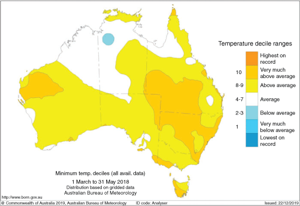
Across mainland Australia, minimum temperatures for autumn 2018 were very much warmer than the historical seasonal average (Fig. 27). Almost all states and territories reported autumn mean minimum areal averages that were ranked in the top-ten for autumn, aside from the Northern Territory (which was still, overall, anomalously warm) and Queensland (with the southern districts also warmer). Tasmania recorded a positive anomaly overall, but the statewide anomalies were closer to average. The rank and anomaly values for each state and territory for autumn 2018 are listed in Tables 4 and 5.

|

|

|
For autumn 2018 (Fig. 28), very much above average night-time temperatures were recorded in southwestern Queensland and northwestern New South Wales as well as the coastal fringe between South Australia, the Gascoyne region in Western Australia and southwestern Tasmania. Minimum temperatures above the seasonal mean for autumn occurred across the south of the continent, along the eastern coastal fringe of Queensland’s Cape York Peninsula, the coastal fringe of the Top End in the Northern Territory and an area south of the Gulf of Carpentaria away from the coast along the Northern Territory’s eastern flank. In an area of the Kimberley in Western Australia, cooler than historical autumn average night-time temperatures were recorded. For the most part, however, northern Australia recorded near-average seasonal daily minimum mean temperatures for autumn 2018.18
|
10 Southern hemisphere
The austral autumn 2018 was again significantly warmer over much of the southern hemisphere. In fact, it was one of the warmest autumns on record for land, ocean and combined. The season ranked as the second-warmest for land (over the period spanning 139 years). For land and ocean combined it was the warmest, and the sixth warmest autumn for the ocean area alone. The continental temperature anomalies, derived from the NOAA Global Temp data set, indicated South America recorded its third-warmest autumn on record, Africa its fourth-warmest and Oceania its fifth-warmest for autumn 2018.19
Temperatures in autumn 2018 were above the long-term average over most of the southern hemisphere land areas outside Antarctica (Fig. 29). Areas that recorded temperatures below the 1981–2010 average were Ecuador, parts of western Peru, central Chile and northeast Brazil. An area around Cape Town, western South Africa and the central west coast of Western Australia also recorded temperatures just below the long-term average. Slightly negative temperature anomalies were also evident around parts of the Antarctic Peninsula. Persistent trade winds were likely responsible for the region of below average temperatures about parts of the northern South Atlantic and Indian Ocean (where autumn mean temperatures were 0.5–1.5°C below average). In March 2018, New Zealand experienced its sixth-warmest March since national records began in 1909 at 1.3°C above the 1981–2010 average.20
|
Temperatures remained above average across much of subequatorial South America during April, 21and data concluded continental temperatures were the highest since 1910. Argentina had its warmest April since national records began in 1961. This value surpassed the previous record set in 1970 by +0.6°C. During the month, several locations set new April mean temperature records that were warmer than the monthly mean. Of note, the city of Buenos Aires set a new April mean temperature record, which was 1.1°C warmer than the historical average, and an April mean daily minimum temperature record with an anomaly above the April average (+2.0°C).22 The May areal average temperature for Argentina was its seventh warmest since 1961.23 Several locations across the country set new maximum temperature records for the month of May. Of note, was a city in the north of the country at latitude 26.783°S, called Presidencia Roque Saenz Peña where a new record was set for daily maximum temperature with 36.6°C recorded on 3 May 2018.
Global rainfall patterns for autumn 2018 (Figs 30, 31) show below average rainfall for autumn over southern South Africa, adding to the rainfall deficiencies experienced in the austral winters of 2015–2017 (Archer et al. 2019). Some parts of central South Africa recorded rainfall that was 25–50% wetter than average in autumn 2018. The South African monsoon season runs from October to April. This area recorded above average precipitation during March and April, with area-averaged totals near the 70th percentile of occurrences.24 Parts of Kenya also received their highest March–May rainfall totals in the last 50 years. The heavy rains displaced almost one million people and caused scores of fatalities.25

|

|
Argentina experienced its ninth-driest March on record and warmer than average March temperatures, which affected much of South America. The northeastern and central regions of Argentina experienced rainfall that was significantly below average, leading to the emergence of serious deficiencies and this impacted the production of soybeans and corn, both important export crops, with significantly reduced yield for the season. Autumn 2018 rainfalls (Fig. 30), were 25–50% lower than average. Some parts of Argentina saw 50–75% lower than average rainfall for this season.
For autumn 2018, some western Pacific island nations received rainfall that was above the historical seasonal mean, due in part to tropical cyclone activity over the southwest Pacific basin. Following the wetter than normal summer 2017–18 for much of New Zealand, autumn 2018 remained generally wetter than normal in the east of both the North Island and the South Island.
Conflicts of interest
The authors declare that they have no conflicts of interest.
Acknowledgement
The authors would like to thank Tamika Tihema and Tony Wedd for reviewing an earlier manuscript; their comments provided an opportunity to significantly improve the manuscript. Naomi Benger is thanked for her helpful final inspection and Blair Trewin for his patience. This research did not receive any specific funding.
References
Archer, E., Landman, W., Malherbe, J., Tadross, M., and Pretorius, S. (2019). South Africa’s winter rainfall region drought: A region in transition? Climate Risk Manage 25, 100188.| South Africa’s winter rainfall region drought: A region in transition?Crossref | GoogleScholarGoogle Scholar |
Donald, A, Meinke, H., Power, B., Wheeler, M., and Ribbe, J. (2004). Forecasting with the Madden-Julian Oscillation and the applications for risk management. In ‘International Crop Science Congress (ICSC 2004): New Directions for a Diverse Planet, 26 September–1 October 2004, Brisbane, Australia’. Available at http://www.cropscience.org.au/icsc2004/poster/2/6/1362_donalda.htm
Hendon, H., Thompson, D. W. J., and Wheeler, M. C. (2007). Australian rainfall and surface temperature variations associated with the southern hemisphere annular mode. J. Climate 20, 2452–2467
Huang, B., Thorne, P. W., Banzon, V. F., Boyer, T., Chepurin, G., Lawrimore, J. H., Menne, M. J., Smith, T. M., Vose, R. S., and Zhang, H.-M. (2017). NOAA Extended Reconstructed Sea Surface Temperature (ERSST), Version 5, ncdc:C0092. National Centers for Environmental Information, NESDIS, NOAA, U.S. Department of Commerce.
Kanamitsu, M., Ebisuzaki, W., Woollen, J., Yang, S., Hnilo, J. J., Fiorino, M., Potter, G. L., et al. (2002). NCEP-DOE AMIPII Reanalysis (R–2). Bull. Amer. Meteor. Soc. 83, 1631–1643.
| NCEP-DOE AMIPII Reanalysis (R–2).Crossref | GoogleScholarGoogle Scholar |
Kuleshov, Y., Qi, L., Fawcett, R., and Jones, D. (2009). Improving preparedness to natural hazards: Tropical cyclone prediction for the Southern Hemisphere. Adv. Geosci. 12, 127–143.
| Improving preparedness to natural hazards: Tropical cyclone prediction for the Southern Hemisphere.Crossref | GoogleScholarGoogle Scholar |
Madden, R. A., and Julian, P. R. (1971). Detection of a 40-50 day oscillation in the zonal wind in the tropical Pacific. J. Atmos. Sci. 28, 702–708.
| Detection of a 40-50 day oscillation in the zonal wind in the tropical Pacific.Crossref | GoogleScholarGoogle Scholar |
Madden, R. A., and Julian, P. R. (1972). Description of global-scale circulation cells in the tropics with a 40-50 day period. J. Atmos. Sci. 29, 1109–11023.
| Description of global-scale circulation cells in the tropics with a 40-50 day period.Crossref | GoogleScholarGoogle Scholar |
Madden, R. A., and Julian, P. R. (1994). Observations of the 40-50 day tropical oscillation: a review. Mon. Wea. Rev. 122, 14–837.
| Observations of the 40-50 day tropical oscillation: a review.Crossref | GoogleScholarGoogle Scholar |
Rosemond, K., and Tobin, S. (2018). Seasonal climate summary for the southern hemisphere (autumn 2016): El Niño slips into neutral and a negative Indian Ocean Dipole develops. J. South. Hemisph. Earth Syst. Sci. 68, 125–146.
| Seasonal climate summary for the southern hemisphere (autumn 2016): El Niño slips into neutral and a negative Indian Ocean Dipole develops.Crossref | GoogleScholarGoogle Scholar |
Saji, N. H., Goscami, B. N., Vinayachandran, P. N., and Yamagata, T. (1999). A dipole mode in the tropical Indian Ocean. Nature 401, 360–363.
| A dipole mode in the tropical Indian Ocean.Crossref | GoogleScholarGoogle Scholar | 16862108PubMed |
Santoso, A., Hendon, H, Watkins, A., et al. (2019). Dynamics and Predictability of El Niño–Southern Oscillation: An Australian Perspective on Progress and Challenges. Bull. Amer. Meteor. Soc. 100, 403–420.
| Dynamics and Predictability of El Niño–Southern Oscillation: An Australian Perspective on Progress and Challenges.Crossref | GoogleScholarGoogle Scholar |
Tihema, T. (2019). Seasonal climate summary for the southern hemisphere (summer 2017–18): An exception-ally warm season for Australia; a short-lived and weak La Niña. J. South. Hemisph. Earth Syst. Sci. 69, 351–368.
| Seasonal climate summary for the southern hemisphere (summer 2017–18): An exception-ally warm season for Australia; a short-lived and weak La Niña.Crossref | GoogleScholarGoogle Scholar |
Tobin, S. (2020). Seasonal climate summary for the southern hemisphere (spring 2017): equal-fifth warmest spring on record, with rainfall mixed. J. South. Hemisph. Earth Syst. Sci. , .
| Seasonal climate summary for the southern hemisphere (spring 2017): equal-fifth warmest spring on record, with rainfall mixed.Crossref | GoogleScholarGoogle Scholar |
Trewin, B. (2018a). Seasonal climate summary for the southern hemisphere (winter): a strong negative Indian Ocean Dipole brings wet conditions to Australia. J. South. Hemisph. Earth Syst. Sci. 68, 101–123.
Trewin, B. (2018b). ‘The Australian Climate Observations Reference Network – Surface Air Temperature (ACORN-SAT)’, version 2. (National Library of Australia: Canberrra, ACT)
Troup, A. (1965). The Southern Oscillation. Quart. J. Roy. Meteor. Soc. 91, 490–506.
| The Southern Oscillation.Crossref | GoogleScholarGoogle Scholar |
Wang, G., and Hendon, H. (2007). Sensitivity of Australian rainfall to inter-El Niño variations. J. Climate 20, 4211–422.
| Sensitivity of Australian rainfall to inter-El Niño variations.Crossref | GoogleScholarGoogle Scholar |
Wheeler, M., and Hendon, H. (2004). An All-Season Real-Time Multivariate MJO Index: Development of an Index for Monitoring and Prediction. Mon. Wea. Rev. 132, 1917–32.
| An All-Season Real-Time Multivariate MJO Index: Development of an Index for Monitoring and Prediction.Crossref | GoogleScholarGoogle Scholar |
1 The Troup SOI (Troup, 1965) used in this article is 10 times the standardised monthly anomaly of the difference in MSLP between Tahiti and Darwin. The calculation is based on 60-year climatology (1933–1992), with records commencing in 1876. The Darwin MSLP was provided by the Bureau of Meteorology, and the Tahiti MSLP was provided by Météo France inter-regional direction for French Polynesia.
2 ENSO 5VAR was developed by the Bureau of Meteorology and is described in Kuleshov et al. (2009). The principal component analysis and standardisation of this ENSO index is performed over the period 1950–1999.
3 SST indices were obtained from ftp://ftp.cpc.ncep.noaa.gov/wd52dg/data/indices/sstoi.indices.
4 http://www.bom.gov.au/climate/iod/
5 http://www.bom.gov.au/climate/mjo/
6 NOAA National Centers for Environmental information, Climate at a Glance: Global Time Series, published May 2017. Available at http://www.ncdc.noaa.gov/cag/ (base period 1900-present).
7 Bureau of Meteorology, Climate Monitoring and Prediction, www.bom.gov.au (internal reference source: from The Analyser)
8 Special Climate Statement No. 64 – record warmth in the Tasman Sea, New Zealand and Tasmania, published 27 March 2018, Bureau of Meteorology and NIWA. Available at http://www.bom.gov.au/climate/current/statements/scs64.pdf
9 Scott, M. 2019. Understanding Climate: Antarctic sea ice extent. Available at https://www.climate.gov/news-features/understanding-climate/understanding-climate-antarctic-sea-ice-extent [accessed 28 September 2019]
10 NOAA National Centers for Environmental Information, State of the Climate: Global Climate Report for March 2018, published online April 2018. Available at https://www.ncdc.noaa.gov/sotc/global/201803 [accessed 10 October 2019]
11 SAM index from the Climate Prediction Center (CPC), see http://www.cpc.ncep.noaa.gov/products/precip/CWlink/daily_ao_index/aao/aao.shtml.
12 For more information on the Bureau of Meteorology’s ACCESS model, see http://www.bom.gov.au/nwp/doc/access/NWPData.shtml
13 NOAA. 2018. Satellite and Information Service, Rare Subtropical Storm off the coast of Chile. Available at https://www.nesdis.noaa.gov/content/rare-subtropical-storm-coast-chile. [Accessed 1 October 2019]
14 NOAA/NCEP. 2018. Climate Monitoring Bulletin, April 2018, Near Real-Time Ocean/Atmosphere Monitoring, Assessments, and Prediction. Available at https://www.cpc.ncep.noaa.gov/products/CDB/CDB_Archive_pdf/PDF/CDB.apr2018_color.pdf.
15 Chart of tropical cyclone Marcus movement: http://www.bom.gov.au/announcements/sevwx/nt/nttc20180316.shtml
16 Chart of tropical cyclone Nora movement: http://www.bom.gov.au/announcements/sevwx/qld/qldtc20180323.shtml
17 Australian Government Bureau of Meteorology. 2018. Special Climate Statement 65 – Persistent Summer-like heat sets many April records. Available at http://www.bom.gov.au/climate/current/statements/scs65.pdf
18 A subset of the full temperature network is used to calculate the spatial averages and rankings shown in Table 3 (maximum temperature), Table 4 (minimum temperature); and Table 5 this data set is known as ACORN-SAT V2 (Trewin, 2018b) These averages are available from 1910 to the present.
19 NOAA National Centers for Environmental Information. 2018. State of the Climate: Regional Analysis for May 2018. Available at from https://www.ncdc.noaa.gov/sotc/global-regions/201805/[Accessed 2 October 2019]
20 NIWA 2018. NIWA Annual Climate Summary, 2018. Available at https://niwa.co.nz/files/2018_Annual_Climate_Summary-NIWA.pdf
21 https://iridl.ldeo.columbia.edu/maproom/Global/Precipitation/Seasonal.html?T=Mar-May%202018
22 NOAA National Centers for Environmental Information, State of the Climate: Global Climate Report for April 2018, published online May 2018, retrieved on 21 September 2019 from https://www.ncdc.noaa.gov/sotc/global/201804
23 https://www.ncei.noaa.gov/sites/default/files/sites/default/files/march–2018-global-significant-events-map.png
24 https://www.cpc.ncep.noaa.gov/products/CDB/CDB_Archive_pdf/PDF/CDB.mar2018_color.pdf
25 https://reliefweb.int/sites/reliefweb.int/files/resources/ROSEA_180606_Kenya%20Flash%20Update%20%236_final.pdf (OCHA 2018).