

Rain and potential evapotranspiration are the main drivers of yield for wheat and barley in southern Australia: insights from 12 years of National Variety Trials
Edward G. Barrett-Lennard A B , Nicholas George C * , Mario D’Antuono D , Karen W. Holmes A and Phillip R. Ward E F
A
B
C
D
E
F
Abstract
Water is widely assumed to be the factor most limiting the growth of annual crops in rainfed environments, but this is rarely tested at sub-continental scale.
Our study aimed to determine the key environmental and management variables influencing the yield of wheat and barley in the grain-production regions of southern Australia, using data from National Variety Trials.
We used generalised additive models to determine the importance of climatic and management variables on wheat and barley grain yield. We determined the effects of the best one, two or three variables and their interactions.
The aridity index, defined as the ratio of cumulative rainfall to potential evapotranspiration, was the single strongest determinant of grain yield for both crops. Model performance was further improved by separating the aridity index into pre-seasonal and seasonal components. Interestingly, other variables that might be expected to influence yield, such as nitrogen fertilisation and extreme temperatures, had relatively minor effects. A comparison between data collected over two 6-year periods showed that there had been yield gains and increased water-use efficiency with time, especially in wetter environments.
Our findings illustrate the importance of water availability for grain production in this region and suggest opportunities for benchmarking and yield prediction through use of readily available climate data.
Our study reinforces the importance of factors such as water-use efficiency and drought tolerance as goals for cultivar development and agronomic research in wheat and barley. It also highlights the potential of National Variety Trial data as a resource for understanding grain production systems and climate resilience. Further work could explore the value of additional variables and improved weather data.
Keywords: barley, fertiliser application, grain yield, national variety trials, potential evapotranspiration, rainfall, water use efficiency, wheat.
Introduction
Water is considered the primary factor limiting crop productivity in dryland farming systems of southern Australia; as such, water-use efficiency and benchmarking crop yields against it have been instrumental in increasing farm productivity in these regions (Richards et al. 2013; Hunt et al. 2021). Nevertheless, the yield potential of grain crops in semi-arid regions is also demonstrably influenced by other factors, notably sowing date, other climate variables, soil fertility, soil constraints and disease, as well as by the non-linear interactions between these factors and water supply (Hochman et al. 2009; Passioura and Angus 2010; Hoogmoed et al. 2018; Hochman and Waldner 2020; Lawes et al. 2021). Identifying the primary factors influencing the yield potential and yield variation of grain crops, as well as the nature and magnitude of these factors and their interactions, is essential for informing cultivar development and optimising agronomic management (Hunt et al. 2021; Crespo-Herrera et al. 2022; Cooper and Messina 2023). In addition, climatic changes have already negatively impacted productivity in Australian grain farming, and significant changes to crop varieties and agronomic management may be needed to adapt grain cropping to future climates (Howden et al. 2010; Sudmeyer et al. 2016; Hochman et al. 2017; Cresswell et al. 2021). An in-depth understanding of the drivers of yield is essential for predicting the future impacts of climate change and how farming systems must adapt.
Field data for exploring environmental and management impacts on grain yield
Exploring environmental and management impacts on grain yield via empirical field experiments is challenging given the numbers and types of variables involved, so the primary drivers of crop yield in Australia are most often determined via biophysical simulations validated through targeted field trials and grower surveys (Anderson 1992; Bryan et al. 2014; Lawes et al. 2016, 2021; Chenu et al. 2017). Multi-state, multi-environment trials – which are often long-running, geographically extensive and agro-environmentally diverse – offer an alternative data source for understanding factors responsible for yield variation. In Australia, the National Variety Trials (NVT) program, funded by the Grains Research and Development Corporation (GRDC), an Australian Federal Government statutory authority, conducts multi-environment trials to test the relevant merits of different cultivars of major grain crops throughout Australian grain-growing regions. The NVTs sample a diverse range of climates, seasonal weather conditions, soil types, and management practices, and the data are publicly available. Multi-environment trials have been used to explore the impact of environmental and management variables on crop yield in other regions globally (e.g. George and Lundy 2019; Munaro et al. 2020). Researchers have also used data from the NVTs for this purpose in Australia (e.g. Hoogmoed et al. 2018; Eichi et al. 2020; Chen et al. 2019), but only for selected crops (usually wheat), in geographically limited regions, or for restricted numbers of variables. It is worth investigating whether NVTs can provide further insights into the key environmental and management variables affecting crop yields in Australia.
Estimating and benchmarking yields with climate variables
Given the importance of rainfall as a driver of yield, for 40 years, farmers and advisors in Australia have used simple rules of thumb based on rainfall to estimate yield potential. This has generally been the empirically derived ‘sum of seasonal rainfall’ – the rain that falls between April and October. This was originally proposed by French and Schultz (1984) and extended by Sadras and Angus (2006). In their original paper, French and Schultz (1984) found that wheat yield potential could best be estimated in rainfed environments by accounting for rainfall, soil moisture and evaporation. The approach spurred agricultural researchers to develop better crop-management strategies to achieve the hypothesised greatest crop water-use efficiency. See Sadras (2020) for a further discussion of the legacy of the French and Schulz methods. Several further attempts have proposed other simple rules for estimating potential yield using weather data (e.g. Hunt and Kirkegaard 2012).
When is the growing season?
Southern Australia has a winter-dominated rainfall season, and several issues arise when considering the sum of seasonal rain as the first (and main) variable predicting crop yield. To begin with, when is ‘the growing season’? When French and Schultz (1984) published their paper, the use of no-till practices in southern Australian farming systems, augmented by the use of knock-down herbicides, was not widespread (D’Emden and Llewellyn 2006), so weed control was still partly achieved after the ‘break’ of the season through the use of several tillage operations. Therefore, at that time, it would not have been unusual for crops to be sown between mid-April and early June. Hence, the French and Schultz definition of the growing season from April to October seemed ‘fit for purpose’. Today, however, crops are often sown into dry conditions or very early in the growing season to take advantage of autumn rainfall (Powles and Bowran 2000; D’Emden and Llewellyn 2006). So, rain falling prior to sowing before the start of winter may also be considered part of the ‘seasonal rainfall’ (Oliver et al. 2009; Harries et al. 2022). To this end, Hunt and Kirkegaard (2012) proposed a method that used 0.25 times the summer fallow rainfall (November–March) plus the growing season rainfall after this time.
The impacts of rainfall timing
Another problem with estimating yield based on rainfall alone is that such calculations assume that water is of equal value to crops in space and, to some degree, in time. From the point of view of space, these methods often assume that water has the same value whether it falls in cooler southern locations or warmer, more northerly locations. From the point of view of time, these methods assume that all water that falls within a growing season (whether it be May, July, or October) is of equal value to crop yield and that all rain that falls in summer and autumn (whether in November of the previous year or April) has 25% of the value of any seasonal rain. Each of these propositions can be questioned; for example, rain in warmer, drier locations might be expected to be of greater value to growing crops than rain in cooler, wetter locations. The value of marginal increases in seasonal water to crop growth may be greater at the start and end of the rainfed growing season (when water is more likely to be limited) than in the middle of the growing season (when water is less likely to be limited).
The importance of evapotranspiration
Another issue, related to that above, is that rain is more important in landscapes of high evapotranspirative demand than in landscapes of low evapotranspirative demand (Sadras and Rodriguez 2007; Sadras and McDonald 2011; Sinclair 2020). The importance of considering water in farming systems in terms of evapotranspiration, and evapotranspirative demand, was acknowledged by French and Schultz (1984). The relationship between rainfall and evapotranspiration can indicate environments with low and high water availability relative to plant demand (Budyko 1974; Stephen 2005; Sahin 2012). Any attempt to understand the influence of water on grain production must include potential evapotranspiration in some way.
The influence of other variables
Given the importance of nitrogen to crop productivity, it is often used along with climate variables to estimate and benchmark yields (Hochman et al. 2009, 2016; Gobbett et al. 2017; Hoogmoed et al. 2018; Hochman and Waldner 2020). However, applying more nitrogen to crops in higher rainfall than in lower rainfall locations is common practice to ensure that crops achieve their ‘yield potential’. This means that the effects of rainfall and fertiliser application may be confounded, which should be explored further. Furthermore, we might also expect nitrogen fertilisation to be confounded with other fertilisers. This needs to be considered in data analyses.
Heat stress and frost can also significantly impact yield and variety adaptation of cereals (Farooq et al. 2011; Teixeira et al. 2013; Zheng et al. 2015a; Crimp et al. 2016; Dreccer et al. 2018). For example, the presence or absence of terminal heat stress is a factor used to characterise global wheat mega-environments (Lillemo et al. 2005; Chenu et al. 2011; Dreccer et al. 2018), and across southern Australia, frost events can cause losses of up to AU$700 million in grain production (Crimp et al. 2016). Therefore, extreme temperature events during the growing season should also be considered for predicting and benchmarking grain yield.
Environmental sampling
Our desire to compare the impacts of climate and management on crops raised another issue. The trials conducted by the NVT staff across southern Australia vary in number and location for the different crop species. Comparing the climatic constraints affecting crop species would be legitimate only if the relative frequencies of the various climate, soil and agronomic variables affecting yield were relatively similar between crops. It is unclear whether this is the case.
Aims and objectives of this work
We used generalised additive models (GAMs) to test the relationship between grain yield and environmental and management variables. Chen et al. (2019) demonstrated the strengths of these models as simple and parsimonious decision tools for predicting wheat yield in Australia using environmental and management variables. GAMs offer advantages such as capturing non-linear relationships, ease of interpretation, and the ability to identify hidden patterns in crop–soil–weather interactions (Chen et al. 2019). To quantify the impacts of variables on yield, we used GAMs to determine the effect of a wide range of ‘families’ of relationships involving climatic and agronomic variables, and their interactions, on wheat and barley yields. We sought to identify the smallest subset of environmental and management variables that would explain the greatest yield variation with acceptable accuracy while allowing for easy interpretability and use.
Our paper asks several questions. Question 1: what are the main constraints to yield? Is it sufficient to consider water as the primary constraint to the yield of grain crops in southern Australia, or are other environmental and management variables also having a significant impact, and if so, what are these variables? Question 2: how should the growing season be defined? In this context, what period should the growing season be considered across, particularly in terms of rainfall, but also how should other ‘water-related’ variables, such as evapotranspiration, be considered? Question 3: if important environmental and management variables are identified, can improved methods for predicting and benchmarking yields be developed? Question 4: given that changes in agronomic practice have occurred over time, do these changes matter in seeking to define the factors affecting crop performance? Related to this is Question 5: are individual crop species evaluated across sufficiently similar environments in the NVTs to enable comparisons between the climatic performances of those crops?
To address these questions, we accessed and analysed publicly available data from the Australian NVTs of wheat (Triticum aestivum L.) and barley (Hordeum vulgare L.) from southern Australia (i.e. the states of Western Australia, South Australia and Victoria). Together, these species occupy >70% of the cropping area in the region and are responsible for a quarter of the value of Australian agricultural exports, contributing significantly to globally traded staple grains and international food security (ABARES 2022; FAO 2022).
Materials and methods
Sources of data
The dataset used in this study comprises late-stage variety test results from the Australian NVT program. The program was established in 2005 by the GRDC and aims to assist Australian grain growers in varietal decision-making by providing comparative information on commercially available grain varieties. Data from these trials are publicly available through the NVT website (https://nvt.grdc.com.au/). In total, 1469 trials were accessed (Table 1).
| Species | South-west | South-east | Total | No. of varieties per trial | |
|---|---|---|---|---|---|
| Wheat (main season) | 470 | 448 | 918 | 19–50 | |
| Barley (main season) | 192 | 359 | 551 | 16–33 | |
| Total | 662 | 807 | 1469 |
Our analyses are based on yield data for ‘main-season’ wheat and barley from trials conducted over the 12 years between 2008 and 2019 (Table 1). It was assumed that the yield potential at each site would be best represented by selecting the highest yielding cultivar at each site. The number of different varieties tested at each site varied with crop species; numbers were higher for wheat (19–50) and slightly lower for barley (16–33).
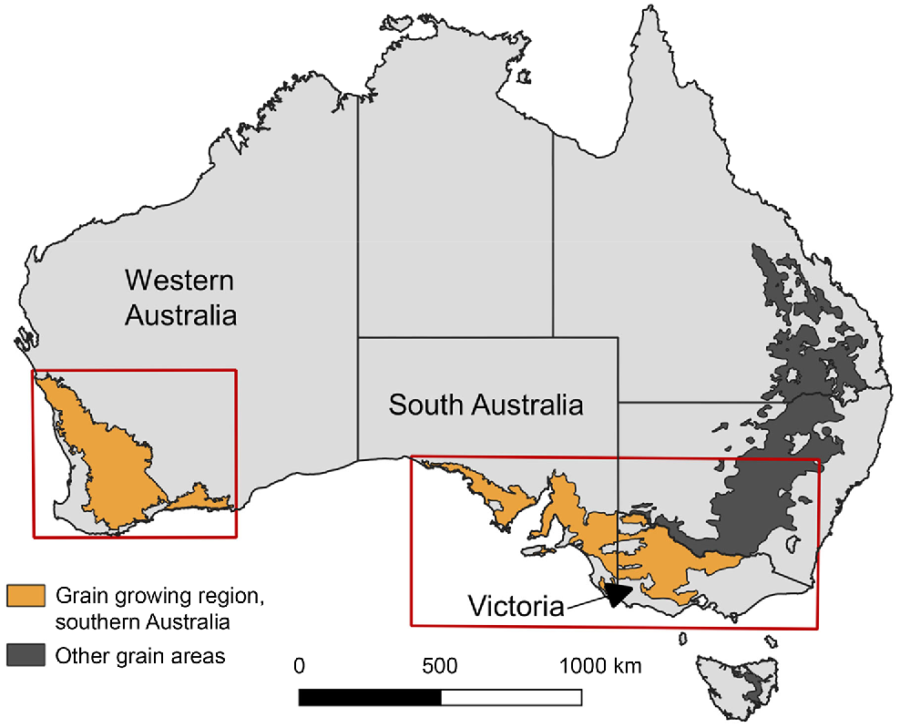
The trials were conducted in the winter rainfall dominant regions of southern Australia (Fig. 1), in the south-west (28.04°–34.77°S, 114.67°–122.27°E) and south-east (31.93°–38.24°S, 133.01°–146.03°E). These trials were reasonably well distributed across both regions. For methodological information, please refer to the NVT website.
Locations of NVTs across southern Australia. The red squares show the two regions, in the south-west and south-east of Australia.
Duplicate trials (i.e. trials grown at the same site in the same year) were sometimes present. These had the potential to distort the dispersion of the data and were removed from the database. We also removed four wheat trials that may have been irrigated (WMaA14NUMU3, WMaA15NUMU3, WMaA16NUMU3 and WMaA17NUMU3).
Climate data for individual trial locations were accessed from the NVT database. Where these were not available, data were obtained from the nearest Bureau of Meteorology weather station (Bureau of Meteorology (BOM) 2023), or the Scientific Information for Land Owners (SILO) database (Jeffrey et al. 2001). The climatic parameters and their codes are listed in Table 2. Monthly sums or monthly averages of climatic variables were estimated as required. We also used the ratio between rainfall and potential evapotranspiration as an estimate of the deficit of water at the locations. We refer to this ratio as the ‘aridity index’; however, unlike more traditional aridity indexes, we applied it to sub-yearly periods (UNEP 1992).
| Variable (units) | Code | Method of calculation | |
|---|---|---|---|
| Sum of rain (mm) | ∑rain | Taken from NVT dataset or nearest BOM weather station; summed over a single month or combination of months | |
| Sum of crop reference evapotranspiration (mm) | ∑ETo | Calculated using the FAO Penman–Monteith formula (Allen et al. 1998); taken from the nearest SILO weather station; summed over a single month or combination of months | |
| Ratio of sum of rain to sum of reference evapotranspiration (mm/mm) | ∑rain/∑ETo | The ratio of the above variables. Here, we refer to this as the ‘aridity index’ (UNEP 1992). This term is usually reserved for annual periods, however, here, we use it for time periods of any length | |
| Sum of pan evaporation | ∑evap | Taken from nearest SILO weather station; summed over a single month or combination of months | |
| Average minimum daily temperature (oC) | av minT | Average minimum temperature measured each day (taken from the nearest SILO weather station); this value averaged over a single month or combination of months | |
| Average maximum daily temperature (oC) | av maxT | Average maximum temperature measured each day (taken from the nearest SILO weather station); this value averaged over a single month or combination of months | |
| Average monthly temperature (oC) | av T | Average of daily maximum and daily minimum temperatures measured each day (taken from the nearest SILO weather station); this value averaged over a single month or combination of months | |
| Temperature range (oC) | range T | Difference between the daily maximum and daily minimum temperatures each day (taken from the nearest SILO weather station); averaged over a single month or combination of months | |
| Highest temperature recorded in a month (oC) | max maxT | Highest daily maximum temperature recorded in a month (taken from the nearest SILO weather station); this value averaged over a single month or combination of months | |
| Lowest temperature recorded in a month (oC) | min minT | Lowest daily minimum temperature recorded in a month (taken from the nearest SILO weather station); this value averaged over a single month or combination of months | |
| Nitrogen fertiliser application (kg/ha) | N fert | Calculated from NVT datasheets | |
| Nitrogen fertiliser applied at (or before) sowing (kg/ha) | N fert start | Calculated from NVT datasheets | |
| Nitrogen fertiliser applied after sowing (kg/ha) | N fert later | Calculated from NVT datasheets | |
| Phosphorus fertiliser (kg/ha) | P fert | Calculated from NVT datasheets | |
| Sulfur fertiliser (kg/ha) | S fert | Calculated from NVT datasheets |
The NVT database also reported other variables that could be related to average crop yield, including the amounts of fertiliser applied. These variables and their codes are also summarised in Table 2. In many trials, nitrogen fertiliser was applied at sowing and on various dates after that. Therefore, we distinguished between the total nitrogen fertiliser applied to the trial, the nitrogen fertiliser applied at sowing, and the nitrogen fertiliser applied after crop establishment.
Statistical analyses
Following the methods of Chen et al. (2019), we used GAMs to establish ‘smoothed’ relationships between the yield of the highest yielding cultivar per site and various combinations of the climatic and the fertiliser variables listed in Table 2. Data manipulation and analyses were performed with R software (R Core Team 2023), and GAMs were performed using the mgcv package (Wood 2017). REML (restricted maximum likelihood) was used for smoothness selection, and to facilitate model selection, an extra penalty was added to each term via the select function in the gam package (Marra and Wood 2011; Wood 2017).
Three models were examined using the additive approach of main effects and interactions. The main modelling syntax in R code is shown below:
where x is an environmental or management variable, s is a smoothed spline fitted to the relationship between x and crop yield, and ti is a tensor product for the interaction between main variable effects. See the documentation for the gam package for further information (Wood 2017).
For Eqn 1, our approach was to build ‘families’ of relationships between crop yield and environmental and management variables. Climatic variables were measured over all possible options of adjacent months. For example, there are 12 possible single months in a year, 11 possible adjacent 2-month periods in a year, 10 possible adjacent 3-month periods, etc. Thus, a family could contain all the sequences of months between January (a sequence of 1 month) and January-to-December (a sequence of 12 months). So, in testing all single-variable relationships between yield and a climatic variable, we calculated the results of 12 + 11 + 10 + 9 + 8 + 7 + 6 + 5 + 4 + 3 + 2 + 1 = 78 possible relationships in a family. For cumulative rain and aridity, we considered the effects of the last 2 months of the previous year (designated Nov.* and Dec.*). So, 14 months were considered giving 14 + 13 + 12 + 11 + 10 + 9 + 8 + 7 + 6 + 5 + 4 + 3 + 2 + 1 = 105 possible relationships in a family. We also considered the value in separating cumulative rain or aridity index into two variables: the first measured over the range of the ‘pre-seasonal’ months between November of the previous year and April (21 options), and the second measured over the range of ‘seasonal’ monthly options from May to October (21 options).
A similar process was used in selecting the optimum two-variable relationships for Eqn 2 except that the number of possible relationship options from within a family could be as high as 105 × 78 = 8190. For Eqn 3, it was not practical to run and filter through more than ~30,000 relationship options at a time, so the range of options assessed was constrained for practicality (see account in Supplementary Materials).
Variables for Eqn 2 were only selected if they accounted for a large proportion of the variation in Eqn 1 (>49% for wheat, >36% for barley), and variables were only used in Eqn 3 if they accounted for a large proportion of the variation in Eqn 2 (>60% for wheat, >47% for barley).
Best relationships in common (across both species) were calculated by aligning the model outcomes for wheat and barley and selecting the combination of months of x-variables (1, 2 or 3) that maximised the adjusted R2 averaged across both species.
Generalised additive models for the ‘best-prospect’ models – those with the largest proportion of variance (adjusted R2) accounted for – identified using the procedures described above were run using the extra penalty function (select = TRUE), which is more conservative than the default, although computationally more intensive (Wood 2017). These final models were then assessed and compared using the Akaike information criterion (AIC), and diagnostic information was generated using the gam.check function in the mgcv package (Wood 2017). The linear relationships between observed and fitted values for all models were assessed using the coefficient of determination (R2), the proportion of variation accounted for by the model, root-mean-square error, slope and intercept. Models were also compared via an analysis of variance to determine whether the more complex model was significantly better than the simpler model (R Core Team 2023). These results were used to select the simplest and most parsimonious model that explained the greatest proportion of yield variation.
Correlations between environmental and management variables can lead to confounding, such that the causal relationships between the variables and yield cannot be established. To test for correlations, a pairwise correlation analysis was performed using the PerformanceAnalytics package (Peterson and Carl 2020). In GAMs, concurvity, the nonparametric analogue to collinearity between terms, occurs when some smooth term in a model can be approximated by one or more of the other smooth terms in the model, which can then lead to an increased risk of type 1 errors (Ramsay et al. 2003; Wood 2017). Therefore, in addition to pairwise correlation analysis, the mgcv package was also used to compute indexes of concurvity between model terms. Once the optimal GAMs were identified using the procedure described above, the predictive power of the final model was tested by k-fold cross-validations, which involved splitting it into random testing and training sets 20 times.
The final selected model was then used to generate figures showing how yield responded to key variable changes. For each variable being assessed, GAMs were used to predict the average point of best fit and the standard error of that value.
Results
Best relationships between climatic variables and yield for each crop, and the calculation of ‘best relationships in common’
The best families of solutions for relationships described in Eqns 1, 2 and 3 are summarised in Table 3. The full range of relationships assessed and a commentary on the process of narrowing from a diverse to a more focused set of relationships is summarised in the Supplementary Materials (see Supplementary Tables S1–S6).
| Crop/GAM relationship | No. of relationships tested in family | Adj. R2 (%) of best relationship | Monthly interval of best relationship | |||
|---|---|---|---|---|---|---|
| x1 | x2 | x3 | ||||
| Wheat | ||||||
| Selected single x-variable relationships: | ||||||
| Hunt and Kirkegaard OK method | ||||||
| 1 | 46.6 | – | – | – | ||
| ∑rain (x1) | ||||||
| 105 | 49.7 | Feb.–Oct. | – | – | ||
| Aridity index (∑rain/∑ETo – x1) | ||||||
| 105 | 54.5 | Feb.–Oct. | – | – | ||
| Selected double x-variable relationships: | ||||||
| ∑rain (pre-seasonal) (x1) × ∑rain (seasonal) (x2) | ||||||
| 21 × 36 | 53.6 | Nov.*–Apr. | May–Oct. | – | ||
| Aridity index (pre-seasonal) (x1) × aridity index (seasonal) (x2) | ||||||
| 21 × 36 | 60.6 | Feb.–Apr. | May–Sept. | – | ||
| Selected triple x-variable relationships: | ||||||
| Aridity index (pre-seasonal) (x1) × aridity index (seasonal) (x2) × av. max. temp. (x3) | ||||||
| 21 × 21 × 78 | 65.6 | Jan.–Apr. | May–Sept. | Apr.–June | ||
| Barley | ||||||
| Selected single x-variable relationships: | ||||||
| Hunt and Kirkegaard OK method | ||||||
| 1 | 33.6 | – | – | – | ||
| ∑rain (x1) | ||||||
| 105 | 36.4 | Nov.*–Oct. | – | – | ||
| Aridity index (∑rain/∑ETo – x1) | ||||||
| 105 | 41.4 | May–Sept. | – | – | ||
| Selected double x-variable relationships: | ||||||
| ∑rain (pre-seasonal) (x1) × ∑rain (seasonal) (x2) | ||||||
| 21 × 36 | 42.0 | Nov.*–Apr. | May–Oct. | – | ||
| Aridity index (pre-seasonal) (x1) × aridity index (seasonal) (x2) | ||||||
| 21 × 36 | 50.6 | Apr. | May–Sept. | – | ||
| Selected triple x-variable relationships: | ||||||
| Aridity index (pre-seasonal) (x1) × aridity index (seasonal) (x2) × av. min. temp. (x3) | ||||||
| 105 × 78 × 1 | 58.1 | Jan.–Apr. | May–Oct. | July–Oct. | ||
The monthly interval of the best climatic variables (*indicates month of previous year) and the number of relationships tested in each family are also presented. The results of these GAM relationships are compared with results using a simple linear fit for the OK method of Hunt and Kirkegaard (2012).
The Hunt and Kirkegaard (2012) method of estimating grain yield from rain, which fits a relationship between grain yield and rainfall (0.25 × ∑rain (Nov.*–Apr.) + ∑rain (May–Oct.)), accounted for the least variation in grain yield in both species (Table 3). Stronger relationships (i.e. with higher adjusted R2 values) were achieved with the others listed in Table 3.
The strength of the relationships increased with increasing number of model terms. Of the single-variable models, the aridity index was the strongest predictor of yield (Table S1). With the two-variable models, either the combination of ∑rain (x1) and ∑ETo (x2) (wheat) or the aridity index separated into pre-seasonal and seasonal components (barley) was the strongest predictor of yield (Table S2). Of the three-variable models, those with the aridity index separated into pre-seasonal and seasonal components, along with extreme temperatures, were the strongest predictor of yield. The average maximum temperature (i.e. the maximum temperature averaged on a daily basis and further averaged over a sequence of months) from April to July was most important for wheat, whereas for barley, the minimum temperature (i.e. the minimum temperature in a month averaged over a sequence of months) between July and October was most important (Table S3). No other climatic variables accounted for more variation or generated more parsimonious models than these.
Despite the attention in the literature that has been placed on the importance of heat stress on crop yields, the highest adjusted R2 values for relationships between elevated temperatures (av maxT or max maxT) and crop yield were 14.0–21.7% less than for the aridity index (Table S1). Nitrogen had the strongest relationship to yield of all the fertilisers, but when considered independently, it explained 27–35% less of the variation in yield than cumulative rainfall (Tables S1 and S4). Furthermore, when nitrogen fertiliser was included along with the aridity index, the percentage of the yield variation explained increased by only 4.6–5.6% relative to the same model without it (Tables S1 and S5).
Final model selection
Tables 4 and 5 present statistics for the selected models and the fit between observed and predicted wheat and barley yields for the GAMs in Table 3. In some cases, the adjusted coefficient of determination presented in Tables 4 and 5 was lower than in Table 3. This is because the GAM model used in the latter tables is more conservative.
| AIC | RMSE | Pearson | Adj. R2 | Slope | Intercept | ||
|---|---|---|---|---|---|---|---|
| Hunt and Kirkegaard (2012) | 2349 | 1.00 | 0.70 | 0.49 | 0.49 | 1.49 | |
| Single-variable models: | |||||||
| ∑rain (Feb.–Oct.) | 2355 | 1.01 | 0.70 | 0.49 | 0.48 | 1.50 | |
| Aridity (Feb.–October) | 2282 | 0.96 | 0.73 | 0.53 | 0.53 | 1.37 | |
| Two-variable models: | |||||||
| ∑rain (pre-seasonal Nov.*–Apr.) and ∑rain (seasonal May–Oct.) (no interaction) | 2319 | 0.98 | 0.72 | 0.51 | 0.51 | 1.43 | |
| ∑rain (pre-seasonal Nov.*–Apr.) and ∑rain (seasonal May–Oct.) (interaction) | 2282 | 0.95 | 0.74 | 0.54 | 0.53 | 1.36 | |
| Aridity (pre-seasonal Feb.–Apr.) and aridity (seasonal May–Sept.) (no interaction) | 2269 | 0.95 | 0.74 | 0.54 | 0.54 | 1.34 | |
| Aridity (pre-seasonal Feb.–Apr.) and aridity (seasonal May–Sept.) (interaction) | 2186 | 0.90 | 0.77 | 0.59 | 0.59 | 1.2 | |
| Three-variable model (final model): | |||||||
| Aridity (pre-seasonal Jan.–Apr.), aridity (seasonal May–Sept.), and av. max. temp. (Apr.–July) (main effects only) | 2204 | 0.91 | 0.76 | 0.58 | 0.58 | 1.23 | |
| Final model with second-order interactions | 2104 | 0.84 | 0.80 | 0.65 | 0.63 | 1.07 | |
| Final model with second- and third-order interactions | 2103 | 0.83 | 0.81 | 0.65 | 0.64 | 1.06 | |
The F-statistic for all models was highly significant (P < 0.001).
AIC, Akaike information criterion; RMSE, root-mean-square error; Pearson, Pearson’s correlation between observed and predicted yield; Adj. R2, adjusted coefficient of determination, or proportion of variance accounted for; Aridity, ∑rain/∑ETo for the specified time interval. *Indicates month of previous season.
| AIC | RMSE | Pearson | Adj. R2 | Slope | Intercept | ||
|---|---|---|---|---|---|---|---|
| Hunt and Kirkegaard (2012) | 1724 | 1.14 | 0.59 | 0.35 | 0.34 | 2.26 | |
| Single variable models: | |||||||
| ∑rain (Nov.*–Oct.) | 1727 | 1.14 | 0.59 | 0.35 | 0.34 | 2.26 | |
| Aridity (May–Sept.) | 1681 | 1.10 | 0.63 | 0.39 | 0.39 | 2.09 | |
| Two variable models: | |||||||
| ∑rain (pre-seasonal Nov.*–Apr.) and ∑rain (seasonal May–Oct.) (no interaction) | 1710 | 1.12 | 0.61 | 0.37 | 0.37 | 2.17 | |
| ∑rain (pre-seasonal Nov.*–Apr.) and ∑rain (seasonal May–Oct.) (interaction) | 1685 | 1.09 | 0.64 | 0.4 | 0.40 | 2.08 | |
| Aridity (pre-seasonal Jan.–Apr.) and aridity (seasonal May–Sept.) (no interaction) | 1671 | 1.08 | 0.64 | 0.41 | 0.41 | 2.03 | |
| Aridity (pre-seasonal Feb.–Apr.) and aridity (seasonal May–Sept) (interaction) | 1617 | 1.01 | 0.70 | 0.49 | 0.48 | 1.80 | |
| ∑rain (Dec.*–Aug.) and ∑ET (Sept.) (no interaction) | 1643 | 1.06 | 0.67 | 0.44 | 0.44 | 1.93 | |
| ∑rain (Dec.*–Aug.) and ∑ET (Sept.) (interaction) | 1644 | 1.05 | 0.67 | 0.44 | 0.44 | 1.93 | |
| Three variable model (final model): | |||||||
| Aridity (pre-seasonal Jan.–Apr.), aridity (seasonal May–Oct.), and min temp (July–Oct.) (main effects only) | 1645 | 1.06 | 0.66 | 0.44 | 0.44 | 1.94 | |
| Final model with second-order interactions | 1603 | 1.01 | 0.70 | 0.49 | 0.48 | 1.77 | |
| Final model with second- and third-order interactions | 1591 | 0.98 | 0.72 | 0.52 | 0.50 | 1.70 | |
The F-statistic for all models was highly significant (P < 0.001).
AIC, Akaike information criterion; RMSE, root-mean-square error; Pearson, Pearson’s correlation between observed and predicted yield; Adj. R2, adjusted coefficient of determination, or proportion of variance accounted for; Aridity, ∑rain/∑ETo for the specified time interval. *Indicates month of previous season.
The simple model using cumulative rainfall had accuracy comparable to the more complex Hunt and Kirkegaard (2012) model in wheat and barley. The model that considered pre-seasonal and seasonal rainfall separately was of comparable accuracy. Considering rainfall and ETo together as the aridity index, either as a single variable or separated into the pre- and post-season, was marginally more reliable than rainfall alone, and for both species the interactions improved the model. The most reliable model used pre-seasonal aridity index, seasonal aridity index, and average maximum temperature (Apr.–July) for wheat and average lowest temperature (July–Oct.) for barley. Including all second- and third-order interactions of main effects resulted in a significantly better model (P < 0.01) than considering only main effects and second-order interactions. There was little or no penalty for including interactions (as determined by AIC). Comparisons between the observed and predicted values from the final model for wheat and barley are shown in the Supplementary Material (Figs S1 and S2).
The correlation analysis between environmental and management variables found significant but weak relationships among the main effects for both species (Figs S3 and S4). The analysis of concurvity between terms in the GAM found weak relationships among main effects that were not considered large enough to necessitate the exclusion of terms (Table S7) (Ramsay et al. 2003; Wood 2017).
Given the well-established agronomic importance of nitrogen and phosphorus, these variables were explored but explained less yield variation than climatic variables; therefore, they are only presented in the Supplementary Material (Tables S4–S6). The correlation analysis showed relatively weak relationships between the climate variables considered in the final models and nitrogen (Figs S3 and S4). Given the additional complexity of the model with nutrients such as nitrogen and phosphorus, the risk of correlation between these and rainfall, and the aim of developing a parsimonious model with as few variables as possible, nitrogen was not included in the final model.
Exploring crop response to water
Table 3 shows that although strong relationships existed between ∑rain or aridity index (x-value) and highest grain yield per site (y-variable), these were not over common intervals of months for the two species. With ∑rain, the adjusted R2 was maximised in wheat when summed over the interval between February and October, whereas in barley, it was maximised when summed over the interval from November of the previous year (Nov.*) to October. With the aridity index, the adjusted R2 was maximised in wheat when summed over the interval between February and October, whereas in barley, it was maximised when summed over the interval from May to September. Therefore, comparisons of responses between crops require us to compromise by selecting a ‘best relationship in common’ that would have been slightly suboptimal for each crop individually.
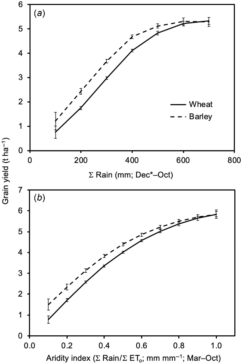
The predicted curves generated using the best relationship in common for single x-variables (∑rain (Dec.*–Oct.) or aridity index (Mar.–Oct.)) are shown in Fig. 2a and b, respectively. The yields of both species decreased as the growing environment became drier or as the aridity index was reduced. At a cumulative rainfall of 100 mm, the predicted yields for wheat and barley were 15% and 23%, respectively, of the predicted yields at 600 mm, and at an aridity index value of 0.1 mm mm−1, the predicted yields were 13% and 26%, respectively, of the predicted yields at 1.0 mm mm−1. Barley had higher yields than wheat under conditions of extreme dryness (∑rain values of 100 mm, aridity index values of ~0.1 mm mm−1).
Smoothed linear representations of the best relationships in common (single x-variable), accounting for variation in highest crop yield per site (y-variable) in wheat and barley: (a) ∑rain (mm, Dec.*–Oct.) as x-variable; (b) aridity index (∑rain/∑ETo, mm mm−1, Mar.–Oct.) as x-variable. Lines denote average fitted values; error bars denote s.e. of the fit. The adjusted R2 values of these relationships are: (a) 49.7% (wheat) and 36.4% (barley); (b) 54.5% (wheat) and 41.4% (barley).
Comparability of wheat and barley datasets
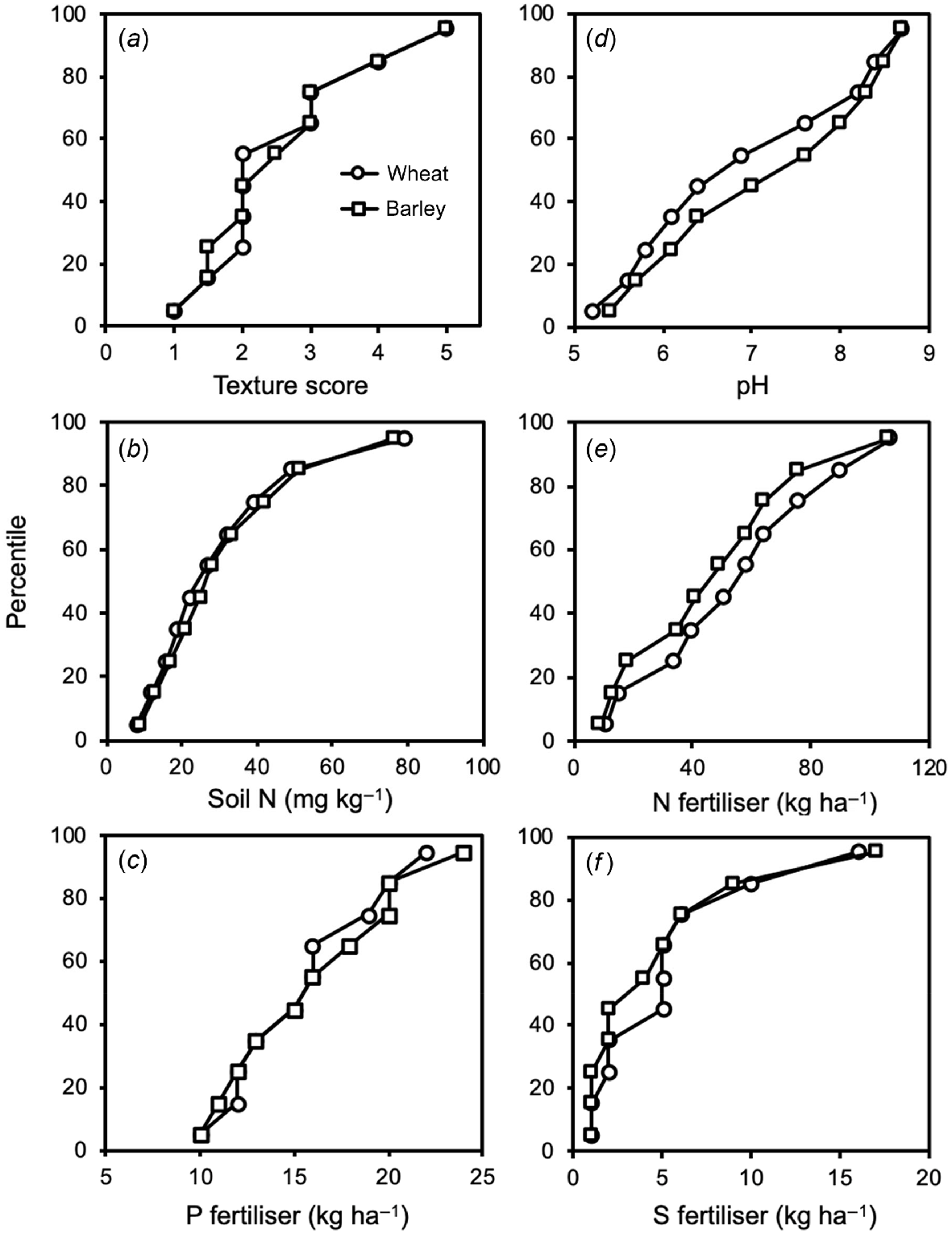
The soil and agronomic variables listed in Table 2 were assessed to identify the relative similarities of the trial sites used for the crops. Table S5 reports the percentile of the distribution of each variable against the level of that variable for wheat and barley, and the number of measurements of each variable for the crops. For most of the variables measured, their distribution across the range of trials was similar between crops, but this was not the case for a few variables (Fig. 3). Where the lines for the two crops were close to each other or overlapped (the case for texture score, soil nitrogen, and phosphorus fertiliser), the trials of the two crops were conducted across similar ranges of conditions. For these, variation in the levels of that variable would not have affected the yield of one crop disproportionately relative to the other. Where the lines differed (the case for pH, nitrogen fertiliser and sulfur fertiliser), the trials were conducted across different ranges of conditions for that variable, and variation might have affected the yield of one crop disproportionately relative to the other.
Graphs of the percentile distribution of a variable against the level of that variable for wheat and barley: (a) texture score at 0–10 cm, (b) soil nitrogen at 0–10 cm, (c) total phosphorus fertiliser, (d) soil pHH2O at 0–10 cm, (e) total nitrogen fertiliser, (f) total sulfur fertiliser. The numbers of trials making up the datasets are indicated in the Supplementary Material (Table S6).
Changes to agronomic practice with time
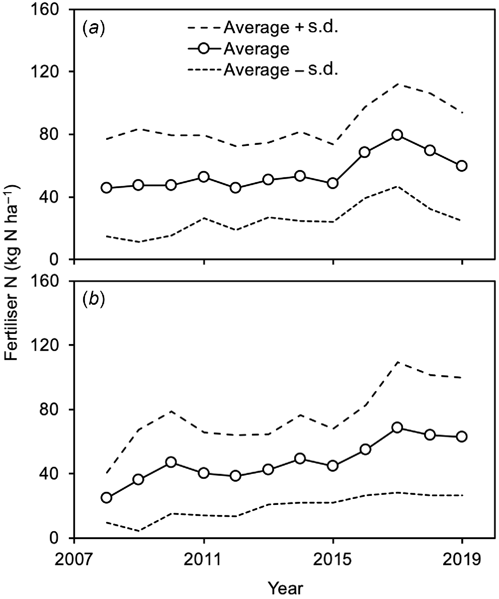
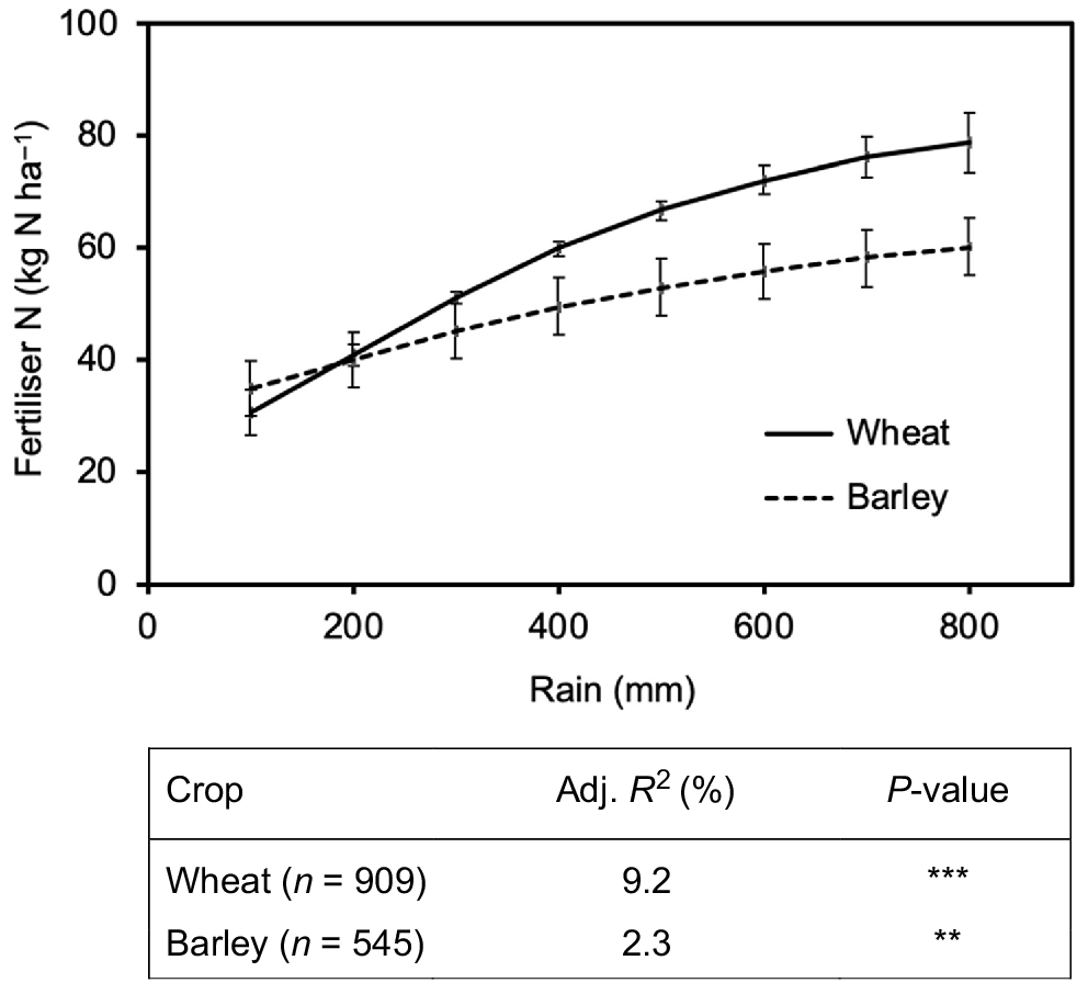
Within years there was wide variation in the amount of fertiliser applied to trials. The coefficient of variation in nitrogen fertiliser application rate varied from 0.41 to 0.77 for wheat and from 0.51 to 0.87 for barley (calculated from data in Fig. 4). However, the rate of nitrogen fertiliser applied to the trials increased with time (Fig. 4). The average amount of nitrogen fertiliser increased by 30% in wheat and 150% in barley during the study period (calculated from data in Fig. 4). Sites of high rainfall received more nitrogen fertiliser than sites of low rainfall, although levels of correlation were not considered large enough to impact the validity of GAMs.
Amounts of nitrogen fertiliser applied to NVTs over the period 2008–2019, aggregated by year of trial, for: (a) main-season wheat, and (b) barley. The points show the average amount of fertiliser applied (n = 909 for wheat, and n = 545 for barley); the dotted lines on either side show this average plus or minus the standard deviation for each year.
The fitted relationship between total rainfall (Dec.*–Oct.) and nitrogen fertiliser rates is presented in Fig. 5. For sites with relatively low rainfall (i.e. ∑rain = 100 mm), the average fertiliser application rates were 30–35 kg N ha−1 for wheat and barley. By contrast, at sites with high rainfall (i.e. ∑rain = 800 mm), the average fertiliser application rates were ~160% and ~70% higher for wheat and barley, respectively, according to district/local practice. In 2008, nitrogen fertiliser was applied mostly at sowing (in 66–69% of cases). However, by 2019, multiple applications of nitrogen fertiliser had become normal practice; only 16–17% of trials received no further nitrogen fertiliser after sowing, with the median trial receiving more than half of its total nitrogen fertiliser application after sowing.
Relationship between ∑rain (Dec.*–Oct.) (x-variable) and the average rate of N fertiliser application (y-variable) applied to NVTs for wheat and barley. Points denote average fitted values; error bars denote s.e. of the fit. The statistics of these relationships are summarised in the table below the graph.
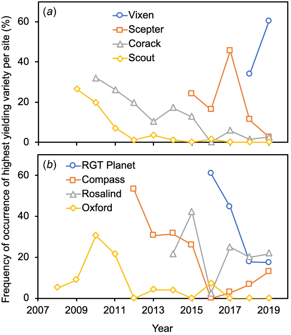
Changes in the highest yielding variety per site and fungicide use were also observed over the 12 years of trials. In 2008–2010, the most important wheat and barley varieties across southern Australia were Scout (highest yielding main-season wheat variety on 27% of sites in 2009) and Oxford (highest yielding barley variety on 31% of sites in 2010) (Fig. 6). By 2017–2019, these had been eclipsed by Vixen (highest yielding main-season wheat variety on 60% of sites in 2019) and RGT Planet (highest yielding barley variety on 44% of sites in 2017). In 2008, an average of seven and five different chemicals-by-application-times were applied to wheat and barley, respectively. By 2019, these numbers had increased to 16 for both species.
Changes in crop yield per site with time
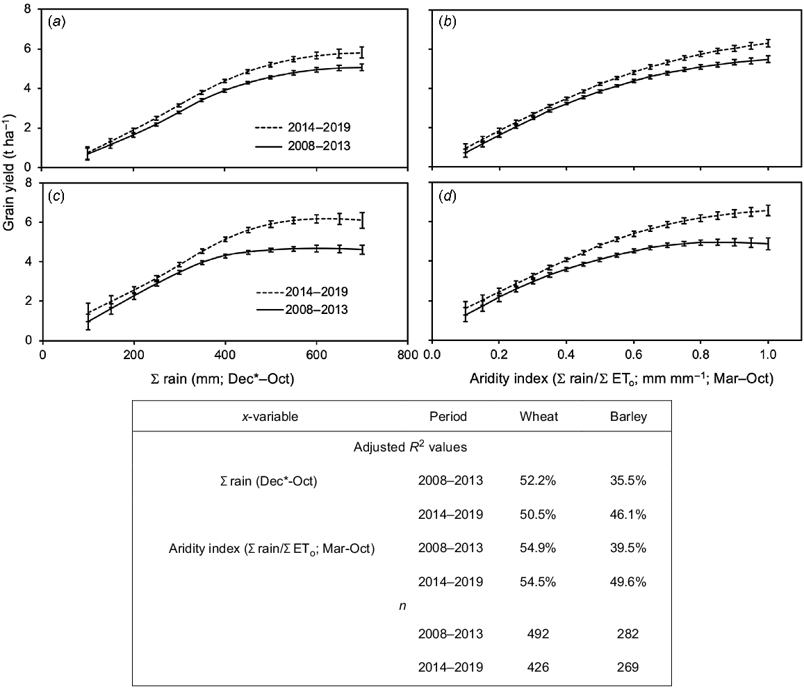
In order to visualise the effects of variety and agronomy changes over the 12 years, the datasets were separated into two 6-year periods (2008–2013 and 2014–2019) (Fig. 7). For both species, the later period had higher crop yields than the earlier period. The difference between the periods was greater at higher rainfall (Fig. 7a, b) or in environments with a higher aridity index (Fig. 7c, d). The average increase in yield between the two 6-year periods was 22% for barley and 11% for wheat (calculated from data in Fig. 7).
Effects of ∑rain (Dec.*–Oct.) or aridity index (∑rain/∑ETo) (x-variables) and the period in which the NVT was conducted (2008–2013 or 2014–2019) on highest crop yield per site for: (a, c) wheat, and (b, d) barley. Each point is a mean predicted from the relevant GAM relationship; error bars denote standard error of the fit. All relationships were significant at P < 0.001. The adjusted R2 of each relationship and the numbers of trials in each set (n) are described in the table below the graph.
Discussion
Our study used the NVT dataset for the two most important field crops grown in southern Australia to test the key variables affecting grain yield. Using GAMs as a statistical tool, we formally analysed the key variables affecting grain yield. Some of our findings are consistent with the outcomes of other studies, for example, the importance of seasonal rainfall (French and Schultz 1984) and including pre-seasonal rainfall (Oliver et al. 2009; Harries et al. 2022). However, our analysis has added new elements and insights (e.g. ETo as a component of the aridity index). We have also formalised the case for these variables driving grain yield in barley and wheat. This paper sought to answer five questions; the following sections refer to each question.
Question 1: what are the main constraints to yield?
Our work has shown that the most important variable accounting for variation in both wheat and barley grain yield in southern Australia is the aridity index (defined here as the ratio of cumulative rainfall to cumulative potential evapotranspiration), either considered as a single variable or separated into a pre-seasonal and seasonal component. A more complex three-variable model considering pre-seasonal and seasonal aridity index, along with extreme temperature (maximum temperature for wheat and minimum temperature for barley), was the most parsimonious model with the greatest explanatory power in both species.
The analysis has also shown that with improved agronomy (i.e. better fertiliser strategies, cultivars, and the use of agricultural chemicals), there were gains in water-use efficiency over the period 2014–2019 compared with 2008–2013. We acknowledge that true water-use efficiency estimates are impossible given the lack of data regarding starting soil moisture. However, starting soil water is likely to be negligible in the winter-rainfall zones of much of southern Australia.
These findings conform to the existing understanding of the primacy of water in dictating grain yield in dryland farming regions of Australia and the validity of a breeding and agronomy focus on water-use efficiency to increase productivity (Richards et al. 2013; Hunt et al. 2021). It also accords with findings that >60% of the variation in global grain yields can be attributed to climatic variation, which in dryland farming regions is predominantly water availability (Ray et al. 2015). Interactions among variables in the final models are significant. However, the biophysical meaning of these interactions is presently unclear and requires further research.
Between about 40% and 50% of yield variation remains unexplained by our best models. Given the known influence of other environmental and management variables on grain yield (Hochman et al. 2009; Passioura and Angus 2010; Asseng et al. 2011; Hoogmoed et al. 2018; Hochman and Waldner 2020; Lawes et al. 2021), it is surprising that inclusion of other factors along with rain and evapotranspiration, such as nitrogen, did not have more explanatory power on their own or improve the predictive power of the model based on water-related variables by more than a few per cent. The possibility of confounding between rainfall and nitrogen fertility was considered, but the lack of correlation between predictors, or concurvity between smoothed terms in the GAMs, suggests that confounding was minimal. There is a perception that NVTs receive ‘luxury’ rates of fertiliser relative to agronomic norms in an area, but there is evidence that NVT sites can be under-fertilised relative to their yield potential (Eichi et al. 2020). We presume that the unexplained variation is due to factors such as fertility, subsoil constraints, disease, and other weather variables. However, this information is either unavailable in the NVT database or is not available with enough precision or accuracy to be useful. For example, the weather from the SILO database is interpolated at the district level (Jeffrey et al. 2001) and may not account well for the weather at a particular field site.
Question 2: how should the growing season be defined?
For many years it has been accepted that seasonal rainfall – defined by French and Schultz (1984) as the rain falling between the months of April and October – is the main variable limiting crop yield in southern Australia and that relationships between seasonal rainfall and crop yield can be described using straight lines. Our analysis finds that the optimal period over which rainfall and evaporation should be considered varies between species. The best models suggest that the pre-season period from January to April needs to be considered in wheat and barley. This finding agrees with Kirkegaard et al. (2007) and Oliver et al. (2009), who found that the rain falling before crops are sown still significantly impacts crop productivity in southern Australia. The seasonal periods for both species are comparable but slightly different, being May–September in wheat and May–October in barley.
Question 3: can improved methods for predicting and benchmarking yields be developed?
Our findings show that the French and Schulz approach of using water to predict and benchmark wheat and barley grain yield in southern Australia remains valid. However, we demonstrate that extending this approach using GAMs including evapotranspiration and appropriate timing of rainfall, and considering other climatic variables, can further improve the accuracy and reliability of the approach. This extends the work of Chen et al. (2019), who argued for using GAMs for simulating wheat yields in Western Australia because of their relative simplicity and ability to capture non-linear relationships and interactions.
Yield response to water availability does not conform to simple linear relationships. It will, of course, be expected to plateau and then decline at higher rainfall as water ceases to limit plant growth. The addition of water exceeding the water-holding capacity of the soil is of limited benefit to plant growth and yield, and excess water can also reduce yields through waterlogging (Oliver et al. 2009). The importance of potential evapotranspiration to plant productivity in natural and agricultural systems is also well established (Sadras and Rodriguez 2007; Sadras and McDonald 2011; Sinclair 2020). Our analyses reinforce the importance of considering potential evapotranspiration when benchmarking crop yields in southern Australia.
Computer-based crop simulation models and decision support tools are important for agricultural research, farm management and extension (Reardon-Smith et al. 2015; Robertson et al. 2015; Ahmed et al. 2016; Muller and Martre 2019; Keating 2020). Several crop models are available, and their performance depends on various factors (Stöckle and Kemanian 2020). The Agricultural Production Systems sIMulator (APSIM), developed by the Agricultural Production Systems Research Unit in Australia, is widely used and has been successfully applied to various crops and agricultural systems globally (Keating et al. 2003; Holzworth et al. 2014; Holzworth et al. 2018). As is the case for many crop models, APSIM requires data that are often not routinely collected or commonly available and is generally not straightforward to use without training, which can be an obstacle to some users (Zheng et al. 2015b; Holzworth et al. 2018; Zhao et al. 2019). This has prompted some workers to find compromises with less complex, but less reliable, models (Chen et al. 2019; Zhao et al. 2019). Furthermore, simple rules of thumb between crop yield and environmental parameters offer a service to farmers, helping them benchmark their crops’ performance for the season. Our work, and that of Chen et al. (2019), demonstrate that GAMs offer a relatively simple tool that can be used to predict grain yield based on widely available climatic input parameters and possibly other variables. We believe that these models could be implemented as a user-friendly software application updated each season with new data from NVTs.
Question 4: do the changes to agronomic practice matter when defining the factors affecting crop performance?
We find substantial evidence for yield gains with time and concomitant improvement in water-use efficiency. However, the gains are greater at higher than at lower levels of water availability. This is in agreement with other work in this field (Harries et al. 2022). Evolution in fertiliser management, along with changes to other practices such as sowing new genotypes and the use of a wider range of herbicides and fungicides, make it challenging for us to attribute yield improvements to any single variable; this is because optimal combinations of technologies have synergistic, not additive, responses (Kirkegaard and Hunt 2010; Kirkegaard 2019; Hunt et al. 2021).
This is also why we have not incorporated the use of fertiliser into our final best relationship in common; given the wide range of simultaneous changes over time in NVTs (fertilisers, genotypes, use of chemicals), it is not safe to attribute the gains to any single factor. If the agronomic changes to trials increase yield potential, then we should find that the lines of best fit between yield and climate parameters would increase with time. Furthermore, as crop yield becomes less limited by crop agronomy and genotype, and more strongly limited by climate, we might expect the gains between yield and climatic variables to decrease with time, with yields becoming increasingly ‘compressed’ against the ceiling created by climate. The higher gain in grain yield in barley than in wheat that we observed may have been partly caused by the increased rates of nitrogen fertiliser applied to barley. For wheat, the average nitrogen application rates over the two 6-year periods were 48 and 62 kg ha−1, a 28% increase. By contrast, for barley, the average rates of nitrogen application were 39 and 57 kg ha−1, respectively, a 46% increase.
Question 5: are individual crop species evaluated across sufficiently similar environments to enable comparisons between the climatic performance of those crops?
In the case of wheat and barley, we found that the species were tested across a sufficiently similar sample of environments and management types to allow direct comparisons and use of similar models. However, care needs to be taken if similar analytical approaches are used for other crop species. For example, it is well known that lupins are grown mainly in lighter soils, limiting our ability to understand the influence of soil type. Wheat and barley are also tested in a relatively large number of environments. Other species are not and, therefore, do not sample such a large diversity of environments and management. This limitation must be considered in any similar use of NVT data.
Concluding remarks and future work
The purpose of the NVTs is to provide crop breeders and farmers with a common and unbiased platform for assessing the relative performance of crop varieties across various environments and seasons, and it has been highly successful in achieving this aim. We have used NVTs as a source of field data to support and extend an understanding of the determinants of yield in southern Australian farming systems. Our work and that of others cited earlier demonstrate the value of the NVTs beyond their original purpose as late-stage variety trials. It shows that making raw data freely and readily available to third-party researchers can deepen the understanding of grain production in Australia to the benefit of Australian farmers and the grains industry. This will increase the value of the investment by the GRDC in the NVTs for little additional cost.
To enhance and extend our work, we believe there is a need to evaluate the reliability and representativeness of the weather data and assess additional environmental and management variables. The weather data we used were interpolated, and it is uncertain whether this accurately reflects the weather at the locations where it was applied. This needs to be investigated further by comparing model reliability for sites with in situ weather stations and those without. Furthermore, potential evapotranspiration was used owing to its availability in the climate databases. Other estimated evapotranspiration measures, such as short-crop evapotranspiration, could be explored as an alternative. We considered all sites in southern Australia in aggregate, but the appropriate interval for rainfall and evapotranspiration may differ between different sub-regions. Finally, variables such as soil profile features, quantitative soil textual information, soil classification, starting soil moisture, date of emergence, weed pressure, disease ratings, and DNA-based testing of soil-borne pathogens may help explain cryptic variation in yield. These variables could be easily obtained from all NVT locations at a relatively low cost with a modest expansion of existing trial protocols. The additional information would not only enhance the value of the trial data for research such as ours but would also increase the overall usefulness of the NVT data and their interpretability. It would also help validate crop models such as APSIM, and better enable use of APSIM to explore more accurately a range of research questions by providing suitable data to initialise the simulation.
Various statistical and machine-learning techniques are increasingly applied to large datasets to determine the nature and magnitude of environmental and genetic influences and their interactions on crop yield (Yan 2014; Lawes et al. 2016; Gogel et al. 2018; Chen et al. 2019; Lawes et al. 2021; Mourtzinis et al. 2021). Although GAMs have advantages in terms of simplicity, other approaches, such as machine learning, could also be applied to the NVT data.
Data availability
The data that support this study were obtained from the website Australian National Variety Trials of the Grains Research and Development Corporation and used with permission.
Acknowledgements
The Grains Research and Development Corporation are sincerely thanked for making National Variety Trial data publicly available. We also thank the various individuals and organisations responsible for implementing the National Variety Trials. We sincerely thank Dr Kefei Chen for his advice on statistical methods and Professor Sally Thompson for advice on ecohydrology.
References
Ahmed M, Akram MN, Asim M, Aslam M, Hassan F-U, Higgins S, et al. (2016) Calibration and validation of APSIM-Wheat and CERES-Wheat for spring wheat under rainfed conditions: models evaluation and application. Computers and Electronics in Agriculture 123, 384-401.
| Crossref | Google Scholar |
Allen RG, Pereira LS, Raes D, Smith M (1998) Crop evapotranspiration - Guidelines for computing crop water requirement. FAO Irrigation and Drainage Paper 56, 300 pp. (Food and Agriculture Organization of the United Nations: Rome, Italy) Available at: https://data.longpaddock.qld.gov.au/static/publications/Evapotranspiration_overview.pdf
Anderson WK (1992) Increasing grain yield and water use of wheat in a rainfed Mediterranean type environment. Australian Journal of Agricultural Research 43, 1-17.
| Crossref | Google Scholar |
Asseng S, Foster I, Turner NC (2011) The impact of temperature variability on wheat yields. Global Change Biology 17, 997-1012.
| Crossref | Google Scholar |
Bryan BA, King D, Zhao G (2014) Influence of management and environment on Australian wheat: information for sustainable intensification and closing yield gaps. Environmental Research Letters 9, 044005.
| Crossref | Google Scholar |
Bureau of Meteorology (BOM) (2023). Australian Government. Available at www.bom.gov.au/climate/data
Chen K, O’Leary RA, Evans FH (2019) A simple and parsimonious generalised additive model for predicting wheat yield in a decision support tool. Agricultural Systems 173, 140-150.
| Crossref | Google Scholar |
Chenu K, Cooper M, Hammer GL, Mathews KL, Dreccer MF, Chapman SC (2011) Environment characterization as an aid to wheat improvement: interpreting genotype–environment interactions by modelling water-deficit patterns in North-Eastern Australia. Journal of Experimental Botany 62, 1743-1755.
| Crossref | Google Scholar | PubMed |
Chenu K, Porter JR, Martre P, Basso B, Chapman SC, Ewert F, et al. (2017) Contribution of crop models to adaptation in wheat. Trends in Plant Science 22, 472-490.
| Crossref | Google Scholar | PubMed |
Cooper M, Messina CD (2023) Breeding crops for drought-affected environments and improved climate resilience. The Plant Cell 35, 162-186.
| Google Scholar | PubMed |
Crimp SJ, Zheng B, Khimashia N, Gobbett DL, Chapman S, Howden M, et al. (2016) Recent changes in southern Australian frost occurrence: implications for wheat production risk. Crop & Pasture Science 67, 801-811.
| Crossref | Google Scholar |
Dreccer MF, Fainges J, Whish J, Ogbonnaya FC, Sadras VO (2018) Comparison of sensitive stages of wheat, barley, canola, chickpea and field pea to temperature and water stress across Australia. Agricultural and Forest Meteorology 248, 275-294.
| Crossref | Google Scholar |
D’Emden FH, Llewellyn RS (2006) No-tillage adoption decisions in southern Australian cropping and the role of weed management. Australian Journal of Experimental Agriculture 46, 563-569.
| Crossref | Google Scholar |
Eichi VR, Okamoto M, Garnett T, Eckermann P, Darrier B, Riboni M, et al. (2020) Strengths and weaknesses of national variety trial data for multi-environment analysis: a case study on grain yield and protein content. Agronomy 10, 753.
| Crossref | Google Scholar |
FAO (2022) FAOSTAT. Food and Agriculture Organization of the United Nations. Available at www.fao.org/faostat/en/#data
Farooq M, Bramley H, Palta JA, Siddique KHM (2011) Heat stress in wheat during reproductive and grain-filling phases. Critical Reviews in Plant Sciences 30, 491-507.
| Crossref | Google Scholar |
French RJ, Schultz JE (1984) Water use efficiency of wheat in a Mediterranean-type environment. I. The relation between yield, water use and climate. Australian Journal of Agricultural Research 35, 743-764.
| Crossref | Google Scholar |
George N, Lundy M (2019) Quantifying genotype x environment effects in long-term common wheat yield trials from an agroecologically diverse production region. Crop Science 59, 1960-1972.
| Crossref | Google Scholar |
Gobbett DL, Hochman Z, Horan H, Navarro Garcia J, Grassini P, Cassman KG (2017) Yield gap analysis of rainfed wheat demonstrates local to global relevance. The Journal of Agricultural Science 155, 282-299.
| Crossref | Google Scholar |
Gogel B, Smith A, Cullis B (2018) Comparison of a one- and two-stage mixed model analysis of Australia’s National Variety Trial South Region wheat data. Euphytica 214, 44-1-44-21.
| Google Scholar |
Harries M, Flower KC, Renton M, Anderson GC (2022) Water use efficiency in Western Australian cropping systems. Crop & Pasture Science 73, 1097-1117.
| Crossref | Google Scholar |
Hochman Z, Waldner F (2020) Simplicity on the far side of complexity: optimizing nitrogen for wheat in increasingly variable rainfall environments. Environmental Research Letters 15, 114060.
| Crossref | Google Scholar |
Hochman Z, Holzworth D, Hunt JR (2009) Potential to improve on-farm wheat yield and WUE in Australia. Crop & Pasture Science 60, 708-716.
| Crossref | Google Scholar |
Hochman Z, Gobbett D, Horan H, Garcia JN (2016) Data rich yield gap analysis of wheat in Australia. Field Crops Research 197, 97-106.
| Crossref | Google Scholar |
Hochman Z, Gobbett DL, Horan H (2017) Climate trends account for stalled wheat yields in Australia since 1990. Global Change Biology 23, 2071-2081.
| Crossref | Google Scholar |
Holzworth DP, Huth NI, deVoil PG, Zurcher EJ, Herrmann NI, McLean G, et al. (2014) APSIM – Evolution towards a new generation of agricultural systems simulation. Environmental Modelling & Software 62, 327-350.
| Crossref | Google Scholar |
Holzworth D, Huth NI, Fainges J, Brown H, Zurcher E, Cichota R, et al. (2018) APSIM next generation: overcoming challenges in modernising a farming systems model. Environmental Modelling & Software 103, 43-51.
| Crossref | Google Scholar |
Hoogmoed M, Neuhaus A, Noack S, Sadras VO (2018) Benchmarking wheat yield against crop nitrogen status. Field Crops Research 222, 153-163.
| Crossref | Google Scholar |
Hunt J, Kirkegaard J (2012) A guide to consistent and meaningful benchmarking of yield and reporting of water-use efficiency. p. 8. Sustainable Agriculture, CSIRO. Available at https://publications.csiro.au/rpr/download?pid=csiro:EP156113&dsid=DS2
Hunt JR, Kirkegaard JA, Harris FA, Porker KD, Rattey AR, Collins MJ, et al. (2021) Exploiting genotype × management interactions to increase rainfed crop production: a case study from south-eastern Australia. Journal of Experimental Botany 72, 5189-5207.
| Crossref | Google Scholar | PubMed |
Jeffrey SJ, Carter JO, Moodie KB, Beswick AR (2001) Using spatial interpolation to construct a comprehensive archive of Australian climate data. Environmental Modelling & Software 16, 309-330.
| Crossref | Google Scholar |
Keating BA (2020) Crop, soil and farm systems models – science, engineering or snake oil revisited. Agricultural Systems 184, 102903.
| Crossref | Google Scholar |
Keating BA, Carberry PS, Hammer GL, Probert ME, Robertson MJ, Holzworth D, et al. (2003) An overview of APSIM, a model designed for farming systems simulation. European Journal of Agronomy 18, 267-288.
| Crossref | Google Scholar |
Kirkegaard JA (2019) Incremental transformation: success from farming system synergy. Outlook on Agriculture 48, 105-112.
| Crossref | Google Scholar |
Kirkegaard JA, Hunt JR (2010) Increasing productivity by matching farming system management and genotype in water-limited environments. Journal of Experimental Botany 61, 4129-4143.
| Crossref | Google Scholar | PubMed |
Kirkegaard JA, Lilley JM, Howe GN, Graham JM (2007) Impact of subsoil water use on wheat yield. Australian Journal of Agricultural Research 58, 303-315.
| Crossref | Google Scholar |
Lawes RA, Huth ND, Hochman Z (2016) Commercially available wheat cultivars are broadly adapted to location and time of sowing in Australia’s grain zone. European Journal of Agronomy 77, 38-46.
| Crossref | Google Scholar |
Lawes R, Chen C, Whish J, Meier E, Ouzman J, Gobbett D, et al. (2021) Applying more nitrogen is not always sufficient to address dryland wheat yield gaps in Australia. Field Crops Research 262, 108033.
| Crossref | Google Scholar |
Lillemo M, van Ginkel M, Trethowan RM, Hernandez E, Crossa J (2005) Differential adaptation of CIMMYT bread wheat to global high temperature environments. Crop Science 45, 2443-2453.
| Crossref | Google Scholar |
Marra G, Wood SN (2011) Practical variable selection for generalized additive models. Computational Statistics & Data Analysis 55, 2372-2387.
| Crossref | Google Scholar |
Mourtzinis S, Esker PD, Specht JE, Conley SP (2021) Advancing agricultural research using machine learning algorithms. Scientific Reports 11, 17879.
| Crossref | Google Scholar |
Muller B, Martre P (2019) Plant and crop simulation models: powerful tools to link physiology, genetics, and phenomics. Journal of Experimental Botany 70, 2339-2344.
| Crossref | Google Scholar |
Munaro LB, Hefley TJ, DeWolf E, Haley S, Fritz AK, Zhang G, et al. (2020) Exploring long-term variety performance trials to improve environment-specific genotype × management recommendations: a case-study for winter wheat. Field Crops Research 255, 107848.
| Crossref | Google Scholar |
Oliver YM, Robertson MJ, Stone PJ, Whitbread A (2009) Improving estimates of water-limited yield of wheat by accounting for soil type and within-season rainfall. Crop & Pasture Science 60, 1137-1146.
| Crossref | Google Scholar |
Peterson BG, Carl P (2020) PerformanceAnalytics: econometric tools for performance and risk analysis. Available at https://CRAN.R-project.org/package=PerformanceAnalytics
R Core Team (2023) ‘R: a language and environment for statistical computing.’ (R Foundation for Statistical Computing: Vienna, Austria) Available at https://www.R-project.org/
Ramsay TO, Burnett RT, Krewski D (2003) The effect of concurvity in generalized additive models linking mortality to ambient particulate matter. Epidemiology 14, 18-23.
| Crossref | Google Scholar | PubMed |
Ray DK, Gerber JS, MacDonald GK, West PC (2015) Climate variation explains a third of global crop yield variability. Nature communications 6, 5989.
| Crossref | Google Scholar | PubMed |
Reardon-Smith K, Mushtaq S, Farley HS, Cliffe N, Stone RC, Ostini J, et al. (2015) Virtual discussions to support climate risk decision making on farms. Journal of Economic and Social Policy 17, 7.
| Google Scholar |
Richards RA, Hunt JR, Kirkegaard JA, Passioura JB (2013) Yield improvement and adaptation of wheat to water-limited environments in Australia – a case study. Crop & Pasture Science 65, 676-689.
| Crossref | Google Scholar |
Robertson MJ, Rebetzke GJ, Norton RM (2015) Assessing the place and role of crop simulation modelling in Australia. Crop & Pasture Science 66, 877-893.
| Crossref | Google Scholar |
Sadras VO (2020) On water-use efficiency, boundary functions, and yield gaps: French and Schultz insight and legacy. Crop Science 60, 2187-2191.
| Crossref | Google Scholar |
Sadras VO, Angus JF (2006) Benchmarking water-use efficiency of rainfed wheat in dry environments. Australian Journal of Agricultural Research 57, 847-856.
| Crossref | Google Scholar |
Sadras VO, Rodriguez D (2007) The limit to wheat water-use efficiency in eastern Australia. II. Influence of rainfall patterns. Australian Journal of Agricultural Research 58, 657-669.
| Crossref | Google Scholar |
Sahin S (2012) An aridity index defined by precipitation and specific humidity. Journal of Hydrology 444–445, 199-208.
| Crossref | Google Scholar |
Sinclair TR (2020) “Transpiration and crop yields” by C.T. de Wit, 1958, Institute of biological and chemical research of field crops and herbage, No. 64.6, Wageningen, the Netherlands. Crop Science 60, 29-31.
| Crossref | Google Scholar |
Stöckle CO, Kemanian AR (2020) Can crop models identify critical gaps in genetics, environment, and management interactions? Frontiers in Plant Science 11, 737.
| Crossref | Google Scholar | PubMed |
Teixeira EI, Fischer G, Van Velthuizen H, Walter C, Ewert F (2013) Global hot-spots of heat stress on agricultural crops due to climate change. Agricultural and Forest Meteorology 170, 206-215.
| Crossref | Google Scholar |
Zhao C, Liu B, Xiao L, Hoogenboom G, Boote KJ, Kassie BT, et al. (2019) A SIMPLE crop model. European Journal of Agronomy 104, 97-106.
| Crossref | Google Scholar |
Zheng B, Chapman SC, Christopher JT, Frederiks TM, Chenu K (2015a) Frost trends and their estimated impact on yield in the Australian wheatbelt. Journal of Experimental Botany 66, 3611-3623.
| Crossref | Google Scholar | PubMed |
Zheng B, Chenu K, Doherty A, Chapman S (2015b) The APSIM-wheat module (7.5R3008). Available at https://www.apsim.info/wp-content/uploads/2019/09/WheatDocumentation.pdf