

Fluorescence in the estimation of chlorophyll-a in public water reservoirs in the Brazilian cerrado
Lucélia Souza de Barros A , Tati de Almeida A , Raquel Moraes Soares A , Bruno Dias Batista B , Henrique Dantas Borges A and Rejane Ennes Cicerelli A B *
A
B
Abstract
The usual strategy for monitoring of eutrophication process is the use of traditional limnological methods, based on laboratory analysis. These procedures involve costly and time-consuming analyses, usually with in vitro methodologies, which can still have limitations in terms of sensitivity and reliability, if poorly managed. Phytoplankton pigments, such as chlorophyll-a (Chl-a), are highly fluorescent and can provide the environmental status of water bodies.
This study aims to analyse, compare and evaluate an estimation of Chl-a through fluorescence in public water sources in the Brazilian cerrado. Exploratory statistical analyses were conducted by using absolute fluorescence units (AFU) and relative fluorescence units (RFU) compared with traditional laboratory data (standard procedure for the determination of Chl-a by spectroscopic methods) to evaluate the significance of differences in estimating Chl-a concentration. Subsequently, empirical models, based on spectral band combinations, were generated to convert fluorescence measurement in Chl-a concentration, by linear regression.
The generated model found a strong correlation and coefficient of determination (r = 0.88; R2 = 0.78). The efficiency of the model was also confirmed by statistical indicators (RMSE = 1.27, MAPE = 26.72 and BIAS = −6.32).
We concluded that the estimate of Chl-a through RFU was better than through AFU.
Therefore, based on the results of this study, it is recommended that RFU be used to obtain more precise and accurate estimates of Chl-a concentration through empirical models based on linear regression.
Keywords: absolute fluorescence units, AFU, aquatic environments, chlorophyll-a, public water supply, relative fluorescence units, RFU, water quality monitoring.
Introduction
Protecting water reservoirs has become critical for maintaining the health of terrestrial ecosystems. In addition to underground sources and rainfall, water that supplies urban and rural areas comes from these surface water bodies. Therefore, it is the responsibility of society to utilise, preserve, and monitor them in a mindful manner (Mustafa et al. 2020). Also, anthropogenic impacts, such as siltation and artificial eutrophication – which are generally caused by point and diffuse source pollution – are progressively worse and more frequent worldwide. These processes’ dynamics are heightened in tropical environments, where the alternation between seasons – hot and humid weather in the summer, followed by a cold and dry period in the winter – lead to an increased capacity for nutrient uptake and consequent rapid growth of algae and aquatic plants (Lewis 2000; Hennemann and Petrucio 2010; Andrade et al. 2020). As a result, some limnological variables may have values out of the adequate water quality range, and the reservoir may fail to fulfil its multiple uses. This is a common scenario in large urban regions, which can make it challenging to establish monitoring strategies that ensure the understanding of the aquatic environment’s dynamics. Chlorophyll-a (Chl-a) is a photosynthetic pigment found in phytoplankton biomass, and it has the potential to serve as a marker for eutrophication, making it an important target with great potential for orientating control measures (Lorenzen 1967; Hartmann et al. 2019; Panchenko et al. 2020).
Currently, there are a variety of approaches to measure and quantify Chl-a. The most traditional and based on laboratory techniques are the spectrophotometric methods and high-performance liquid chromatography (HPLC; Marino 2017; Batista and Fonseca 2018; Garrido et al. 2019). Although these methods provide very reliable quantifications, they are in vitro methods which demand benchtop protocols with several steps and substantial consumption of chemical reagents that can deteriorate algae at the time of extraction (Lorenzen 1967; Van Heukelem and Thomas 2001; Marino 2017; Graban et al. 2020). In addition, analyses are time-consuming, require a large sample volume and involve high logistic and analytical costs (Ferreira et al. 2012; Kuha et al. 2020), which can delay the availability of results and response actions for prevention and control.
To overcome this temporal limitation, alternative technologies that present real-time data acquisition have been proposed (Loisa et al. 2015; Cremella et al. 2018; Shin et al. 2018; Garrido et al. 2019; Panchenko et al. 2020; Silva and Garcia 2021). Fluorescence optical sensors stand out among diverse technologies. Roesler et al. (2017) highlight the benefits of using in vivo fluorescence, such as ease of use, immediate non-destructive determination of concentrations from the organisms, and high rates of data acquisition, precision and accuracy.
This method is based on the spectral ranges of excitation and emission of each pigment. For Chl-a, absorbance wavelengths are smaller than 675 nm (453–440, 620–635 and 672–675 nm) and re-emission is at ~685 nm (Lohrenz et al. 2003; Seppälä et al. 2007; Suggett et al. 2010; Choo et al. 2018; Shin et al. 2020). These ranges (fluorimetric bands) play a very important role in pigment detection and identification of algae groups. Ling et al. (2018) showed good results using fluorescence emission channels at 550 and 700 nm to estimate Chl-a and to distinguish microalgae groups. Garrido et al. (2019) also had good results with this method, but used other fluorimetric bands (370, 450, 525, 570, 590 and 610 nm) for pigment quantification. Despite these advantages, some studies report concerns regarding acquired data, such as observed by Catherine et al. (2012), which identified overestimated Chl-a values when compared to traditional laboratory measurements.
Besides, many other works, with different approaches, also evaluated the effectiveness of in vivo fluorescence determination (Leboulanger et al. 2002; Gregor and Maršálek 2004; Richardson et al. 2010; Houliez et al. 2012; Kring et al. 2014; Escoffier et al. 2015; Ling et al. 2018; Hartmann et al. 2019). However, several of these were developed in either controlled environments, temperate regions, or in sites with high Chl-a concentrations, which differ from tropical reservoirs that can be highly heterogeneous in comparison.
Considering the above, the present study aims to analyse and evaluate methods of Chl-a estimation by fluorescence in reservoirs for public water supply in the cerrado region (Brazil). To this end, different compositions in terms of absolute and relative fluorescence units (emission and excitation regions) were tested to assess their accuracy in detecting Chl-a. We believe that raw fluorometric data (relative fluorescence units, RFU) can be adapted through empirical models, which could improve the process of estimating Chl-a in specific environmental conditions.
Material and methods
Experimental area
The aquatic environments studied in this work are in the cerrado, a biome located in central Brazil, known to contain most of the headwaters of the country’s main hydrographic basins (Lima 2011). Its climate is characterised by a dry season and a rainy season, with an average annual precipitation in the range of 800–1800 mm and average temperatures ranging between 20 and 27°C (Pereira et al. 2011).
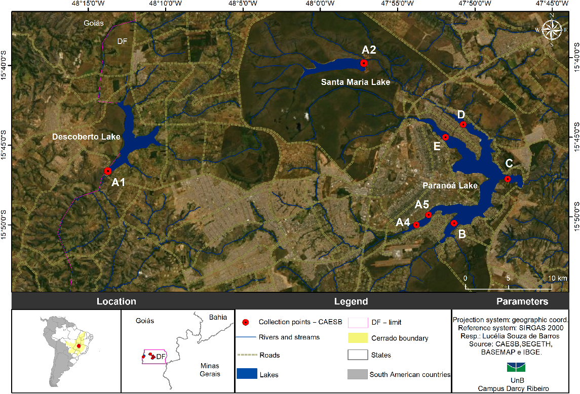
The study was carried out in three public water reservoirs in the Federal District (FD): Descoberto, Santa Maria and Paranoá lakes (Fig. 1), which supply water to ~3 million people (IBGE 2017). Descoberto lake accounts for 60% of the public water supply and is in the western region of the FD, with useful volume of 86 ×106 m3 (Governo do Distrito Federal 2017). Over the years, expansion of agricultural activity and inadequate occupations of its surroundings has been contributing to its pollution. The second studied reservoir – Santa Maria – is located in a conservation area, the National Park of Brasília, that occupies an area of 6.1 km2 with a grassland–cerrado landscape. According to the Integrated Planning for Addressing the Water Crisis (Governo do Distrito Federal 2017), the Descoberto and Santa Maria reservoirs have been suffering from low levels of precipitation (drought) in recent years, which has interfered with catchment levels. This situation pushed the FD Environmental Sanitation Company (CAESB) to interrupt the water supply, which required a rotation distribution system for FD regions in 2016 and 2017.
The 2016–2017 water crisis led to an emergency use of Paranoá lake as a source of water to public supply. Also, in 2016, along with the water crisis, the same lake recorded high nutrient concentrations that resulted in eutrophication and, consequently, the emergence of an intense cyanobacteria growth, which can be harmful to the environment and to human health (Barbosa et al. 2019). Thus, Paranoá lake was chosen as the third study site. This multiple-uses water body, located in FD’s central region, with an area of ~48 km2, is heavily influenced by the anthropic activities in its surroundings, particularly by receiving treated wastewater effluents. The reservoirs were sampled for analyses with the same design sample due to the fact that concentration range of Chl-a was very similar among them. This is justified by the proximity between them, as well as similar environmental and meteorological conditions.
Data acquisition design and estimation methods
In this study, data acquisition was carried out along with the routine sampling done by the CAESB, that carries out systematic water quality monitoring using conventional methods. The sampling points and dates (covering ~1 year of data collection) are listed in Table 1 and Fig. 1. The variation on depths was dependent on routine sampling done by the CAESB, without affecting the results. Kiefer et al. (1989) demonstrated that, depending on the wavelength, the quality of fluorescence is relatively constant with the depth.
| Date | Points | Reservoir | Depths | Number of samples | |
|---|---|---|---|---|---|
| 10 July 2019 | A1 | Descoberto (area 12 km2) | 30 cm (surface) | 1 | |
| 21 October 2019 | 30 cm, 1 m, and 5 m | 3 | |||
| 15 August 2019 | A2 | Santa Maria (area 7 km2) | 30 cm (surface) | 1 | |
| 19 June 2019 | C, D, and E | Paranoá (area 38 km2) | 1 m | 3 | |
| 23 July 2019 | D, and E | 2 | |||
| 13 August 2019 | A4, A5, B, C, D, and E | 6 | |||
| 22 October 2019 | 6 | ||||
| 19 November 2019 | 6 | ||||
| 11 December 2019 | 6 | ||||
| 11 February 2020 | 6 | ||||
| 17 August 2020 | A5, B, C, D, and E | 30 cm | 5 (validation) | ||
| Total | 45 |
Concentration of chlorophyll-a was estimated by two different methods: a traditional spectrophotometric technique (reference) and in vivo fluorescence (IVF) by spectrofluorometer (portable probes). The traditional estimation method used for validation was performed by the CAESB, using the 10200 H reference technique of the Standard Methods for the Examination of Water and Wastewater (American Public Health Association et al. 2012).
Each water sample collected in the field was kept under refrigeration and in the dark until arrival at the laboratory, where they were filtered through a Whatman GF/F filter (porosity 0.7 μm and diameter 47 mm) and frozen. These were then subjected to pigment extraction with a 90% acetone solution. Samples were then analysed using a spectrophotometer at 664 and 750 nm and then, after acidifying with a 0.1-N HCl solution, re-analysed at 665 and 750 nm. This methodology has been used in Brazilian inland waters by several authors (Ferreira et al. 2012; Utsumi et al. 2015; Silva et al. 2016; Cicerelli et al. 2017).
Chlorophyll-a concentration was also measured using spectrofluorometry by IVF. These instruments induce specific excitation (absorption) and emission (fluorescence) wavelengths by directing a beam of light (light-emitting diode, LED) at a specific wavelength and then measuring the highest fluorescence wavelength emitted (Yellow Springs Inc. 2009). In this study, two models were tested: the multi-parameter probe EXO2 from YSI and the bbe Moldaenke FluoroProbe (ver. 2.6 E2, bbe Moldaenke, Schwentinental, Germany). According to the EXO2-YSI manufacturer’s standard procedure for Chl-a estimation, the excitation wavelength occurs at 470 ± 15 nm, whereas the emission wavelength is at 685 ± 20 nm. For the estimation of the phycocyanin and phycoerythrin pigments, the excitation wavelength is at 590 and 525 ± 15 nm respectively, and the emission wavelength is at 685 ± 20 nm (Choo et al. 2018). The FluoroProbe fluorometer has six excitation wavelengths – 370, 470, 525, 570, 590 and 610 nm – with an emission wavelength range between 685 and 700 nm. The results are generated in RFU, that is a unit of measurement used in analysis which employs fluorescence detection. Also, it should be noted that these instruments provide Chl-a estimate in absolute fluorescence units (AFU, μg L−1).
Then, using the localisation from each point of the design sample (Fig. 1), we acquired chlorophyll concentration by traditional limnologic method and the fluorescence method. The probes remained recording data for 4 min with 2-s intervals. The fluorescence data were used to obtain an average of each point. As stated above, the EXO probe gave us only AFU (μg L−1) to compare with the reference value.
Modelling and statistical analysis
Chlorophyll-a data acquired by the fluorometers (μg L−1) as well as by the traditional laboratory analyses (in vitro) were subjected to an exploratory statistical evaluation. First, a basic descriptive statistical analysis of the data was performed, followed by normality tests (Shapiro–Wilk and Kolmogorov–Smirnov tests), which identified data that did not fit the normal distribution. A boxplot visualisation was then used to investigate the source of the abnormality, which could have arisen from outliers, noisy observations, or abnormal system behaviour (Díaz Muñiz et al. 2012; Gradilla-Hernández et al. 2020). Frequently, a raw dataset may contain data with atypical behaviour (outliers), so it is important to categorise the outlier type to adopt the best data refinement strategy (Gradilla-Hernández et al. 2020). It was concluded that many of the observed outliers were caused by common limnologic variation in aquatic environments; consequently, these observations were not excluded.
Previous studies also did not find normal distributions for similar datasets and used non-parametric statistics to perform comparative analyses, such as the Spearman correlation (Hartmann et al. 2019) and the Kruskal–Wallis test (Garrido et al. 2019). In this work, the Kruskal–Wallis test and Dunn’s post hoc (or Dunn–Bonferroni) pairwise comparative method were used to analyse and compare the differences between the evaluated methods. Furthermore, data analysis was complemented by other metrics: linear regression, 95% reliability, probability of significance (P-value), correlation, coefficient of determination (R2) and root mean square error (RMSE), with the aim of evaluating the behavior, accuracy, dispersion and trend of AFU compared with reference data.
The chosen approach for relative fluorescence data analysis was then used to develop empirical models by combining emission spectra bands, to estimate Chl-a concentrations from fluorometric measurements, similarly to what is described in Ling et al. (2018). These authors also applied a method based on combinations of fluorescence emission spectra bands to estimate dominant algal species in marine environments.
In this study, after several tests, eight combinations were used, which included individual band analysis and bands ratio operations (Table 2). For each combination of fluorescence emission, all 40 collected samples were used to create the model. Pearson correlation (r), determination coefficient (R2) and dispersion analysis were used to determine the best model. Subsequently, regression analysis was used to generate Chl-a estimation models from the relationship between laboratory spectrophotometry data and relative fluorescence data. These models considered dispersion of the points in relation to the regression function, with a 95% confidence interval and a P-value of 0.05. The model that had the best statistical results was chosen to estimate Chl-a.
| Band combinations | ID | |
|---|---|---|
| Individual band x | (1) | |
| log10(x) | (2) | |
| (x)−(y) | (3) | |
| (x) ÷ (y) | (4) | |
| log10(x) ÷ log10(y) | (5) | |
| [(x)−(y)] ÷ [(x) ÷ (y)] | (6) | |
| [(x)−(y)] ÷ [(y) ÷ (x)] | (7) | |
| [(x) + (y)] ÷ [(x) ÷ (y)] | (8) | |
| [(x) + (y)] ÷ [(y) ÷ (x)] | (9) | |
| [(x)−(y)] ÷ [(x) + (y)] | (10) |
Data validation
Statistical analyses were performed to assess the performance and accuracy of the chosen model. Three statistical indicators, commonly used in limnological variables research, were applied: RMSE, mean absolute percentage error (MAPE) and systematic error (BIAS) (Ling et al. 2018; Kuha et al. 2020). These can be calculated as follows:
To evaluate model performance, another dataset was collected in situ on 17 August 2020 (5 points), and Chl-a values, determined by the model, were compared with values obtained by the traditional spectrophotometric technique.
Owing to the small quantity of validation points, the validation technique ‘leave-one-out cross-validation’ was also applied to provide an overall assessment of the model accuracy. However, it does not evaluate the dependence of the estimation error on Chl-a values. Such an evaluation, for the estimation error associated with the uncertain model parameters, can be achieved through a non-parametric bootstrap method (Efron 1979; Volpe et al. 2011). As such, we adopt a bootstrap resampling method, in which the observed set of Chl-a fluorescence pairs are re-sampled with re-substitution (i.e. a pair that has been extracted is available for possible subsequent sampling).
Results and discussion
Absolute fluorescence units
Fieldwork was carried out in favourable boating weather conditions of temperature (average 22°C), wind (average 1.1 m s−1), air humidity (55%) and with no rain. Statistical analyses of the Chl-a concentration absolute values provided by the fluorometers are shown in Table 3. All the values were below 30 μg L−1 in the evaluated period, which is within the limit established by the Brazilian environmental regulations Resolução n°357, de 17 de Março de 2005 (Ministério do Meio Ambiente e Mudança do Clima 2005). Although observed values were low, data variability was still observed, as shown by the standard deviation values. The coefficients of variation obtained from fluorometers EXO2 and bbe Moldaenke were of 118 and 86% respectively. Laboratory analyses (LAB) provided the smallest variability values (66%).
| Variable | EXO probe | BBE probe | LAB | |
|---|---|---|---|---|
| Sample size | 40 | 40 | 40 | |
| Min. | 0.28 | 1.60 | 0.80 | |
| Max. | 10.01 | 20.88 | 11.8 | |
| Total amplitude | 9.73 | 19.28 | 11 | |
| Median | 0.88 | 3.92 | 3.60 | |
| Average | 1.89 | 5.63 | 4.09 | |
| Variance | 5.02 | 23.56 | 7.50 | |
| s.d. | 2.24 | 4.85 | 2.74 | |
| s.e. | 0.35 | 0.77 | 0.43 | |
| Coefficient of variation | 118.73% | 86.15% | 66.91% |
According to Table 3, average Chl-a concentration was lower than 6 μg L−1 for all methods. By contrast, other works in the literature that used similar methods, such as the papers by Gregor et al. (2005), Catherine et al. (2012) and Garrido et al. (2019), found medium values of 90, 265 and 42 μg L−1 respectively. It seems clear that estimation under these conditions is difficult, as it is close to the detection limit of the techniques employed.
The Kruskal–Wallis non-parametric test showed significant difference (P < 0.05) between the three tested methods. However, when compared in pairs with the Dunn method, there was no significant difference between the LAB and the BBE measurement (P-adjusted < 0.05), differently for measurements by LAB and EXO (P-adjusted < 0.05). Fig. 2 shows the outlier points (7, 6 and 1 for EXO2, BBE and LAB methods respectively) which were measured at the same date for the sampling sites in each of the three lakes being studied. Thus, it is concluded that the effects of outliers were the result of common phenomena in these aquatic environments.
Distribution of chlorophyll-a (Chl-a) data using fluorimeter (BBE and EXO2) and spectrophotometric (LAB) methods.
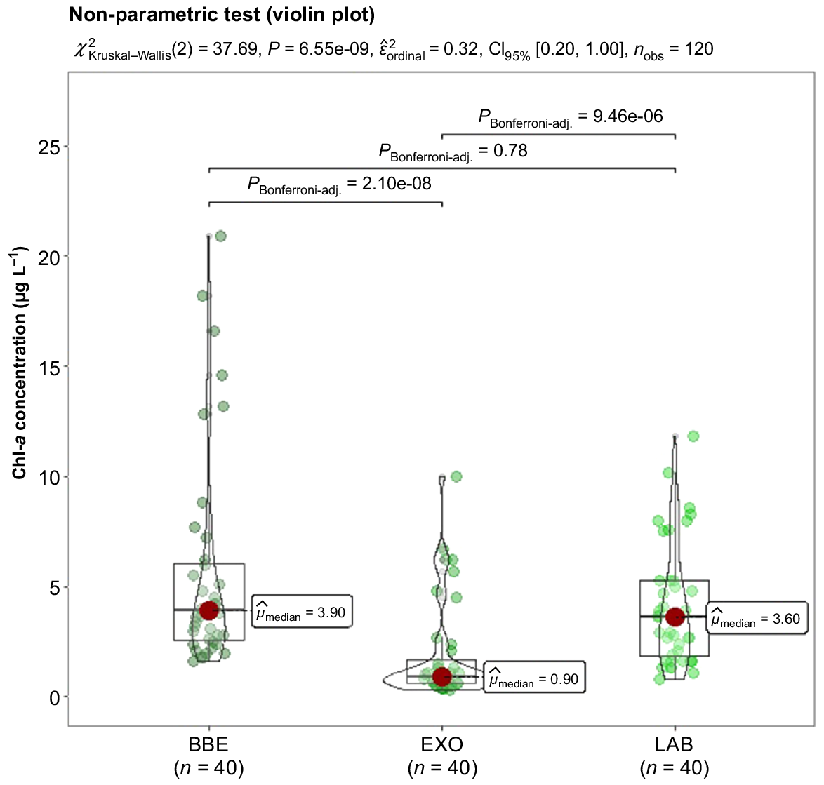
Fig. 2 also shows a violin plot statistical data distribution for every tested method. Chlorophyll-a values from portable fluorometers generally are higher than those obtained by the conventional spectrophotometric technique. This overestimation could have been caused by several reasons, such as an increase in fluorescence emission by cyanobacteria in the face of nutrient limitation (MacIntyre et al. 2010), the phytoplankton life cycle phase and its variations in the pigment content of cells (Beutler et al. 2002), the different levels of efficiency during the extraction of Chl-a by the spectrophotometric method (Nusch 1980), as well as other factors, such as light variation, presence of bubbles, dissolved organic matter, turbidity and temperature (Zamyadi et al. 2016; Choo et al. 2018). Besides considering the type and size of the algae, it is worth mentioning that the fluorescence method predicts the estimation for a point based on a set of data collected over time, taking into account the variation in types and sizes of naturally occurring algae in the environment, as well as their composition, richness and abundance.
This overestimation could have also been caused by the HPLC-based calibration method of the BBE fluorometer, as discussed by Meyns et al. (1994). Several studies have calculated an ‘overestimation index’ for Chl-a spectrofluorometry measurements, with values ranging from 0.27 to 1.03 (Leboulanger et al. 2002; Silva et al. 2016) (Table 4). Additionally, Leboulanger et al. (2002) found a Chl-a concentration and overestimation index similar to what was found in the present study.
| Extraction solvet | Chl-a concentration range (μg L−1) | Number of sampled places | Overestimation factor | Reference | |
|---|---|---|---|---|---|
| Acetone | 0–20 | 1 | 1.03 A | Leboulanger et al. (2002) | |
| Ethanol | 0–50 | 6 | 0.83 A | Gregor and Maršálek (2004) | |
| Ethanol | 0–90 | 5 | 0.74 A | Gregor et al. (2005) | |
| Methanol | 0–265 | 50 | 0.56 B | Catherine et al. (2012) | |
| Ethanol | 42–626 | 1 | 0.36 A and 0.27 B | Silva et al. (2016) | |
| Acetone | 0–20.8 | 3 | 1.37 B | This study |
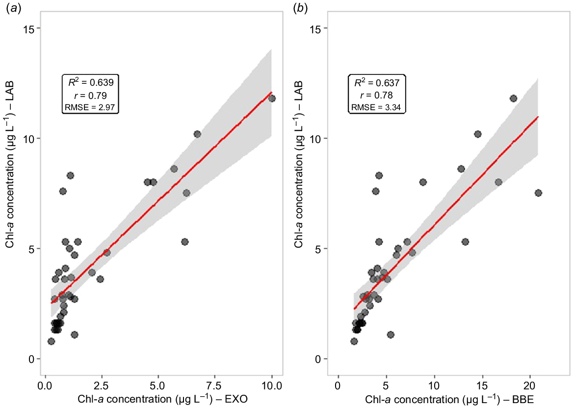
Fig. 3 shows a scatter plot of spectrophotometry (LAB) and spectrofluorometry (EXO and BBE) chlorophyll-a measurements. The LAB and EXO results were strongly correlated (r = 0.79, R2 = 0.63, P < 0.0001, n = 40) and had a relatively low RMSE (2.97). The BBE probe results also show a strong correlation (r = 0.78, R2 = 0.63, P < 0.0001, n = 40), but with a higher RMSE of 3.34. A possible reason for such difference is the due to outliers, as can be seen in Fig. 3b. Concentrations above 5 μg L−1 did not fit well to the linear regression model and can be seen out of the grey zone corresponding to the confidence interval (95%). A different scenario can be seen in Fig. 3a where EXO measurements had a better fit to the linear regression, which can be attributed to these measurements finding Chl-a concentrations below 10 μg L−1.
Linear regression models of the spectrofluorometry methods. (a) Chlorophyll-a (Chl-a) EXO: Y = 2.234 + 0.984X; (b) Chl-a BBE: Y = 1.536 + 0.453X.
Previous studies, such as Silva et al. (2016), found a strong correlation between spectrofluorometry and spectrophotometry methods for Chl-a concentrations bellow 100 μg L−1 (r = 0.84, P < 0.001, n = 25), and a low correlation for concentrations above 100 μg L−1 (r = 0.17, P = 0.63, n = 10). Gregor et al. (2005) and Catherine et al. (2012) also observed strong correlations (r = 0.95, n = 96; r = 0.97, n = 50) for maximum Chl-a concentrations of 90 and 264 μg L−1 respectively. On the other hand, Leboulanger et al. (2002) found a high correlation in an aquatic environment with maximum Chl-a of 20 μg L−1 (r = 0.77, n = 55), which is similar to the present study’s conditions. Those studies show that low biomass frequently provides minor correlation coefficients. Although these studies have found strong correlations, in general factors such as organic matter, total suspended material and bloom conditions in particular, can limit the accuracy of the results (Chang et al. 2012; Kring et al. 2014; Zamyadi et al. 2016).
Relative fluorescence units
Table 5 shows the fluorescence emission bands combination results. Among the various combinations, equation 9, with the 525- and 570-nm bands, had the overall best result, with a Pearson correlation value (r) of 0.88 and a coefficient of determination (R2) of 0.78. In contrast to what was found here, other studies have shown different spectral bands for selective excitation of Chl-a. Suggett et al. (2010), Seppälä et al. (2007) and Lohrenz et al. (2003) used the band combinations of 453–440, 620–635 and 672–675 nm respectively. Blockstein and Yadid-Pecht (2014) also used a different wavelength (465 nm) for the estimation of Chl-a concentrations using a self-made portable, and Gosset et al. (2018) used 470 nm as the excitation wavelength, which is the suggested value to be used with the bbe FluoroProbe fluorometer
| Combinations | r | R2 | Combinations | r | R2 | |
|---|---|---|---|---|---|---|
| 1: (525) | 0.85 | 0.72 | 7: (525–570) ÷ (570 ÷ 525) | 0.85 | 0.73 | |
| 1: (610) | 0.83 | 0.69 | 7: (570–590) ÷ (590 ÷ 570) | 0.83 | 0.69 | |
| 1: (370) | 0.83 | 0.69 | 8: (525 + 590) ÷ (525 ÷ 590) | 0.78 | 0.61 | |
| 1: (590) | 0.86 | 0.73 | 8: (570 + 590) ÷ (570 ÷ 590) | 0.78 | 0.61 | |
| 1: (470) | 0.79 | 0.62 | 8: (610 + 370) ÷ (610 ÷ 370) | 0.79 | 0.62 | |
| 2: (log10 470) | 0.79 | 0.63 | 8: (610 + 590) ÷ (610 ÷ 590) | 0.86 | 0.74 | |
| 2: (log10 525) | 0.83 | 0.69 | 8: (370 + 470) ÷ (370 ÷ 470) | 0.77 | 0.60 | |
| 2: (log10 610) | 0.83 | 0.70 | 9: (525 + 570) ÷ (570 ÷ 525) | 0.88 | 0.78 | |
| 2: (log10 370) | 0.84 | 0.71 | 9: (525 + 590) ÷ (590 ÷ 525) | 0.82 | 0.67 | |
| 2: (log10 590) | 0.85 | 0.73 | 9: (610 + 590) ÷ (590 ÷ 610) | 0.81 | 0.65 | |
| 3: (525–570) | 0.87 | 0.76 | 9: (370 + 590) ÷ (590 ÷ 370) | 0.77 | 0.60 | |
| 3: (590–570) | 0.81 | 0.66 | 9: (525 + 610) ÷ (610 ÷ 525) | 0.78 | 0.61 | |
| 6: (525–570) ÷ (525 ÷ 570) | 0.81 | 0.65 | 9: (370 + 470) ÷ (470 ÷ 370) | 0.86 | 0.73 |
Equation combinations 1, 2, 3, 6, 7, 8 and 9 are those used in Table 2. The bold data are the best results. r, Pearson correlation; R2, coefficient of determination.
The 525- and 570-nm spectral bands, which showed the best results here, are generally related to fluorescence peaks that occur in brown (Bacillariophyceae and Dinophyceae) and mixotrophic (Cryptophyceae) algae groups, which contain accessory pigments, other than chlorophyll-a, such as chlorophyll-c and phycobiliproteins (bbe Moldaenke 2017). Batista and Fonseca (2018) found Bacillariophyceae, Chlorophyceae and Cryptophyceae as the predominant microalgae groups in Paranoá lake, and Roriz et al. (2019) had previously observed the invasive Dinophyceae species Ceratium furcoides (Levander) Langhans in this lake.
In a marine environment, Ling et al. (2018) found good results using fluorescence emission spectral channels at 550 and 700 nm to distinguish marine microalgae, which, along with the present study, corroborates the idea that using flexibly chosen specific spectral channels is a promising approach to the characterisation and quantification of phytoplankton.
Fig. 4 shows the linear regression for model values (fluorometric measurements combinations) and laboratory Chl-a determinations. Results show a high correlation between values (r = 0.88), as well as a good model fit (R2 = 0.77), which show a stronger correlation than what was found by Leboulanger et al. (2002), who obtained r = 0.77 for waters with maximum Chl-a values of 20 μg L−1. However, other studies have shown higher correlation values, such as Gregor et al. (2005) (r = 0.95, n = 96) and Catherine et al. (2012) (r = 0.97, n = 50). Also, it was observed in the present study that relative values provided a better estimate of Chl-a than AFU values (FluoroProbe: R2 = 0.63, r = 0.78).
Linear regression (y = 0.135 + 0.068x) analysis for chlorophyll-a (Chl-a) estimation based on fluorometric measurement combinations and laboratory Chl-a determinations.
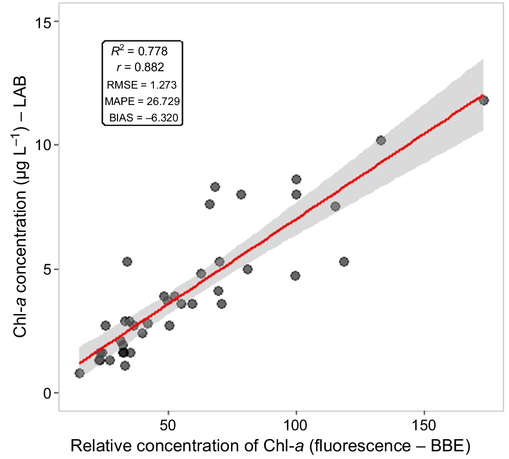
Other indicators, such as the RMSE, MAPE and BIAS, were used to analyse the method’s performance for estimating the concentration of Chl-a. For the best performing model, the statistical values were: RMSE = 1.27, MAPE = 26.72 and BIAS = −6.32 (Fig. 4). The RMSE for RFU was lower than for AFU (BBE probe: RMSE = 3.34). Previous studies from Ferreira et al. (2012) and Ling et al. (2018) also showed the efficiency of fluorescence relative measurements for the quantification and identification of phytoplankton. Both brought improvements to the estimation model.
When converting fluorometric data into relative values of Chl-a, the correction factors may suffer various interferences and cause deviations from the spectrophotometric results. Several authors pointed out that light intensity, temperature, biomass composition and quenching effects can affect the fluorescence responses, resulting in changes in the fluorescence values obtained, which can lead to measurement imprecision (Catherine et al. 2012; Chang et al. 2012; Kring et al. 2014; Cicerelli et al. 2017; Garrido et al. 2019).
For data validation, the model produced by RFU was fed with a dataset obtained in situ on 17 August 2020 (5 points, Table 1) and the results were compared to concentration values obtained from spectrophotometric analyses in the laboratory. The estimated values (1.44–2.65 μg L−1) were very close to laboratory measurements (3.37–0.87 μg L−1), which reinforces the accuracy and precision of the Chl-a estimate model, as confirmed by a RMSE of 0.48 and correlation coefficient (r) of 0.80. The strong correlation, along with a small error value, shows the good performance of the model calibration.
A bootstrap technique was then utilised. In it, the observed set was resampled 10 000 times. This procedure essentially constructs many samples from the same empirical distribution. The resulting empirical distribution of the correlation coefficients (Fig. 4) shows that the values found in the original samples are reliable. The empirical distribution of Pearson’s correlation coefficient presented a median of 0.88 and varied between 0.7922 and 0.9822, with a confidence interval of 95%. These analyses show the high dependence between the concentration of Chl-a and fluorescence data. Regarding the values of β0 and β1, the standard deviation was of 0.005 and 0.389 respectively, highlighting model stability.
The aim of the second validation method, which applied the jackknife technique, was to understand the role of each point in the RFU model, and to verify if the model can predict all the variability in Chl-a concentration. Using this method, generated linear coefficients ranged from −0.022 to 0.210. That is, each model cuts the Y-axis of the cartesian plane in significantly different places. By contrast, the angular coefficient shows a stable behaviour, as there was little variation (0.068–0.073), which indicates a smaller variation of the slope of the line, reinforcing the robustness of the model.
Escoffier et al. (2015) pointed out that, in order to improve estimates, it is important to apply specific fluorimetric calibrations that correspond to the species present in the aquatic environment. However, this can be a complex activity, that is usually carried out directly by equipment manufacturers. The alternative presented in this work, along with what was reported in Ferreira et al. (2012) and Ling et al. (2018), proved to be an excellent quantification tool to estimate Chl-a concentration in aquatic environments using field data calibration.
However, it is worth mentioning the importance of knowing the effects of other environmental factors in Chl-a quantification, as these interferences may vary according to the species or groups of microalgae found in aquatic environments. For instance, a group that has a relatively high concentration can corrupt the determination of another group with lower concentration. Moreover, the model is adapted to specific characteristics of the environment, which means that the model will not be able to adjust to extreme phenomena, such as the occurrence of high concentration of Chl-a or even a mixture of other elements not foreseen in the construction of the regression model.
Conclusions
The correlation between Chl-a estimates from the different methods and the traditional estimate (LAB) was strong, but the presence of outliers affected the linear regression model at concentrations above 5 μg L−1. These results highlight the importance of considering these factors and using appropriate approaches when studying Chl-a concentration in tropical aquatic environments.
In conclusion, the results of fluorimetric measurements (relative data) confirm the efficiency of the model, with a strong correlation (r = 0.88; R2 = 0.78), further supported by validation parameters (RMSE = 1.27, MAPE = 26.72 and BIAS = −6.32). These fluorimetric measurements achieved good estimation accuracy and precision for Chl-a concentration, which is necessary for tropical environments with low concentrations in public water supply reservoirs in the cerrado region. The absolute model provided by manufacturers showed limitations in estimation, which were minimised by using relative models.
The method of combining fluorescence emission bands and the conversion process is a good alternative for the quantification of Chl-a concentration, highlighting the 525- and 570-nm wavelengths corresponding to brown and mixotrophic microalgae. Therefore, relative fluorometric data can be adapted by using empirical models and improving the potential in estimating Chl-a. The estimation model offered by the fluorometers’ manufacturers, which is based on absolute values, should be improved, or adapted to tropical regions, and that is dependent on the predominant phytoplankton groups in the environment.
This alternative allows fast Chl-a quantification because the fluorescence results in less time and work in the analysis in the laboratory, which is a relevant factor for monitoring the water quality in the reservoirs. In addition, there is a reduction in operating costs, ease of use, stability, ease of equipment transportation and a small carbon footprint. Freshwater ecosystems researchers have an accurate and easy way to determine Chl-a concentration.
Data availability
The data that support this study will be shared upon reasonable request to the corresponding author.
Declaration of funding
This work was supported by grants from Financiadora de Estudos e Projetos (FINEP) through the Project ‘CT-HIDRO 01/2013 – AQUAVANT’ (number 01.14.0114.00), from Fundação de Apoio à Pesquisa do Distrito Federal (FAP-DF) through the projects ‘Monitoramento da Qualidade da Água nos Reservatórios do Distrito Federal Utilizando Imagens Obtidas por VANT e por Plataformas Orbitais’ (number 17457.78.36995.26042017) and ‘Dinâmica da Qualidade da Água nos reservatórios do Distrito Federal (DF) por meio imagens obtidas por RPAs e por plataformas orbitais’ (number 00193.00001143/2021-15), and by the Coordenação de Aperfeiçoamento de Pessoal de Nível Superior - Brasil (CAPES) (finance code 001).
References
Andrade EM, Ferreira KCD, Lopes FB, Araújo ICS, Silva AGR (2020) Balance of nitrogen and phosphorus in a reservoir in the tropical semiarid region. Revista Ciência Agronômica 51(1), e20196800.
| Crossref | Google Scholar |
Barbosa JSB, Bellotto VR, da Silva DB, Lima TB (2019) Nitrogen and phosphorus budget for a deep tropical reservoir of the Brazilian Savannah. Water 11, 1205.
| Crossref | Google Scholar |
Batista BD, Fonseca BM (2018) Fitoplâncton da região central do Lago Paranoá (DF): uma abordagem ecológica e sanitária: Phytoplankton in the central region of Paranoá Lake, Federal District of Brazil: an ecological and sanitary approach. Engenharia Sanitária e Ambiental 23, 229241 [In Portuguese with English title and abstract].
| Crossref | Google Scholar |
bbe Moldaenke (2017) FluoroProbe III: the instrument for depth profiles of microalgae. (bbe Moldaenke: Schwentinental, Germany) Available at https://www.bbe-moldaenke.de/en/products/chlorophyll/details/fluoroprobe.html?file=files/knowledge-media/brochures/FluoroProbe_eng.pdf [Verified 19 January 2024]
Beutler M, Wiltshire KH, Meyer B, et al. (2002) A fluorometric method for the differentiation of algal populations in vivo and in situ. Photosynthesis Research 72, 39-53.
| Crossref | Google Scholar | PubMed |
Blockstein L, Yadid-Pecht O (2014) Lensless miniature portable fluorometer for measurement of chlorophyll and CDOM in water using fluorescence contact imaging. IEEE Photonics Journal 6(3), 6600716.
| Crossref | Google Scholar |
Catherine A, Escoffier N, Belhocine A, Nasri AB, Hamlaoui S, Yéprémian C, Bernard C, Troussellier M (2012) On the use of the FluoroProbe, a phytoplankton quantification method based on fluorescence excitation spectra for large-scale surveys of lakes and reservoirs. Water Research 46(6), 1771-1784.
| Crossref | Google Scholar | PubMed |
Chang D-W, Hobson P, Burch M, Lin T-F (2012) Measurement of cyanobacteria using in-vivo fluoroscopy – effect of cyanobacterial species, pigments, and colonies. Water Research 46, 5037-5048.
| Crossref | Google Scholar |
Choo F, Zamyadi A, Newton K, Newcombe G, Bowling L, Stuetz R, Henderson RK (2018) Performance evaluation of in situ fluorometers for real-time cyanobacterial monitoring. H2Open Journal 1, 26-46.
| Crossref | Google Scholar |
Cicerelli RE, Galo MLBT, Roig HL (2017) Multisource data for seasonal variability analysis of cyanobacteria in a tropical inland aquatic environment. Marine and Freshwater Research 68(12), 2344-2354.
| Crossref | Google Scholar |
Cremella B, Huot Y, Bonilla S (2018) Interpretation of total phytoplankton and cyanobacteria fluorescence from cross-calibrated fluorometers, including sensitivity to turbidity and colored dissolved organic matter. Limnology and Oceanography: Methods 16, 881-894.
| Crossref | Google Scholar |
Díaz Muñiz C, García NPJ, Alonso Fernández JR, Martínez Torres J, Taboada J (2012) Detection of outliers in water quality monitoring samples using functional data analysis in San Esteban estuary (Northern Spain). Science of The Total Environment 439(15), 54-61.
| Crossref | Google Scholar |
Efron B (1979) Bootstrap methods: another look at the jackknife. The Annals of Statistics 7(1), 1-26.
| Crossref | Google Scholar |
Escoffier N, Bernard C, Hamlaoui S, Groleau A, Catherine A (2015) Quantifying phytoplankton communities using spectral fluorescence: the effects of species composition and physiological state. Journal of Plankton Research 37(1), 233-247.
| Crossref | Google Scholar |
Ferreira RD, Barbosa CCF, Novo EMLM (2012) Assessment of in vivo fluorescence method for chlorophyll-a estimation in optically complex waters (Curuai floodplain, Pará – Brazil). Acta Limnologica Brasiliensia 24(4), 373-386.
| Crossref | Google Scholar |
Garrido M, Cecchi P, Malet N, Bec B, Torre F, Pasqualini V (2019) Evaluation of FluoroProbe performance for the phytoplankton-based assessment of the ecological status of Mediterranean coastal lagoons. Environmental Monitoring and Assessment 191, 204.
| Crossref | Google Scholar | PubMed |
Gosset A, Durrieu C, Renaud L, Deman A-L, Barbe P, Bayard R, Chateaux J-F (2018) Xurography-based microfluidic algal biosensor and dedicated portable measurement station for online monitoring of urban polluted samples. Biosensors and Bioelectronics 117, 669-677.
| Crossref | Google Scholar | PubMed |
Governo do Distrito Federal (2017) Plano Integrado de Enfrentamento à Crise Hídrica. Governo de Brasília, Special Publication Number 1. (GDF: Brasília, Brazil) Available at https://www.agenciabrasilia.df.gov.br/wp-conteudo/uploads/2017/03/plano-integrado-de-enfrentamento-a-crise-hidrica-governo-de-brasilia.pdf [In Portuguese, verified 19 January 2024]
Graban S, Dall’Olmo G, Goult S, Sauzède R (2020) Accurate deep-learning estimation of chlorophyll-a concentration from the spectral particulate beam-attenuation coefficient. Optics Express 28(16), 24214-24228.
| Crossref | Google Scholar |
Gradilla-Hernández MS, de Anda J, Garcia-Gonzalez A, Meza-Rodríguez D, Yebra Montes C, Perfecto-Avalos Y (2020) Multivariate water quality analysis of Lake Cajititlán, Mexico. Environmental Monitoring and Assessment 192(5), 5.
| Crossref | Google Scholar |
Gregor J, Maršálek B (2004) Freshwater phytoplankton quantification by chlorophyll a: a comparative study of in vitro, in vivo and in situ methods. Water Research 38(3), 517-522.
| Crossref | Google Scholar |
Gregor J, Geriš R, Maršálek B, Heteša J, Marvan P (2005) In situ quantification of phytoplankton in reservoirs using a submersible spectrofluorometer. Hydrobiologia 548, 141-151.
| Crossref | Google Scholar |
Hartmann A, Horn H, Röske I, Röske K (2019) Comparison of fluorometric and microscopical quantification of phytoplankton in a drinking water reservoir by a one-season monitoring program. Aquatic Sciences 81(1), 19.
| Crossref | Google Scholar |
Hennemann MC, Petrucio MM (2010) Seasonal phytoplankton response to increased temperature and phosphorus inputs in a freshwater coastal lagoon, Southern Brazil: a microcosm bioassay. Acta Limnologica Brasiliensia 22(3), 295-305.
| Crossref | Google Scholar |
Houliez E, Lizon F, Thyssen M, Artigas LF, Schmitt FG (2012) Spectral fluorometric characterization of Haptophyte dynamics using the FluoroProbe: an application in the eastern English Channel for monitoring Phaeocystis globosa. Journal of Plankton Research 34, 136-151.
| Crossref | Google Scholar |
Instituto Brasileiro de Geografia e Estatística (2017) Censo Demográfico. (IBGE: Brasília, Brazil) Available at https://cidades.ibge.gov.br/brasil/df/brasilia/panorama [In Portuguese, verified 19 January 2024]
Kiefer DA, Chamberlin WS, Booth CR (1989) Natural fluorescence of chlorophyll a: relationship to photosynthesis and chlorophyll concentration in the western South Pacific gyre. Limnology and Oceanography 34, 868-881.
| Crossref | Google Scholar |
Kring SA, Figary SE, Boyer GL, Watson SB, Twiss MR (2014) Rapid in situ measures of phytoplankton communities using the bbe FluoroProbe: evaluation of spectral calibration, instrument intercompatibility, and performance range. Canadian Journal of Fisheries and Aquatic Sciences 71, 1087-1095.
| Crossref | Google Scholar |
Kuha J, Järvinen M, Salmi P, Karjalainen J (2020) Calibration of in situ chlorophyll fluorometers for organic matter. Hydrobiologia 847, 4377-4387.
| Crossref | Google Scholar |
Leboulanger C, Dorigo U, Jacquet S, Le Berre B, Paolini G, Humbert JF (2002) Application of a submersible spectrofluorometer for rapid monitoring of freshwater cyanobacterial blooms: a case study. Aquatic Microbial Ecology 30, 83-89.
| Crossref | Google Scholar |
Lewis WM, Jr (2000) Basis for the protection and management of tropical lakes. Lakes & Reservoirs: Research & Management 5, 35-48.
| Crossref | Google Scholar |
Lima JEFW (2011) Situação e perspectivas sobre as águas do cerrado. Ciência e Cultura 63(3), 27-29 [In Portuguese with English abstract].
| Crossref | Google Scholar |
Ling Z, Sun D, Wang S, Qiu Z, Huan Y, Mao Z, He Y (2018) Retrievals of phytoplankton community structures from in situ fluorescence measurements by HS-6P. Optics Express 26, 30556-30575.
| Crossref | Google Scholar |
Lohrenz SE, Weidemann AD, Tuel M (2003) Phytoplankton spectral absorption as influenced by community size structure and pigment composition. Journal of Plankton Research 25, 35-61.
| Crossref | Google Scholar |
Loisa O, Kaaria J, Laaksonlaita J, Niemi J, Sarvala J, Saario J (2015) From phycocyanin fluorescence to absolute cyanobacteria biomass: an application using in-situ fluorometer probes in the monitoring of potentially harmful cyanobacteria blooms. Water Practice and Technology 10, 695-698.
| Crossref | Google Scholar |
Lorenzen CJ (1967) Determination of chlorophyll and pheo-pigments: spectrophotometric equations. Limnology and Oceanography 12, 343-346.
| Crossref | Google Scholar |
MacIntyre HL, Lawrenz E, Richardson TL (2010) Taxonomic discrimination of phytoplankton by spectral fluorescence. In ‘Chlorophyll a fluorescence in aquatic sciences: methods and applications. Developments in Applied Phycology. Vol. 4’. (Eds DJ Suggett, O Prasil, MA Borowitzka) pp. 129–169. (Springer)
Marino L (2017) Relação entre clorofila-a e cianobactérias no estado de São Paulo: Link between chlorophyll-a and cyanobacteria in the state of São Paulo. Revista DAE 65, 32-43 [In Portuguese with English title and abstract].
| Crossref | Google Scholar |
Meyns S, Illi R, Ribi B (1994) Comparison of chlorophyll-a analysis by HPLC and spectrophotometry: where do the differences come from? Archives für Hydrobiologie 132, 129-139.
| Crossref | Google Scholar |
Ministério do Meio Ambiente e Mudança do Clima (2005) Resolução n°357, de 17 de Março de 2005. (CONAMA) Available at https://conama.mma.gov.br/?option=com_sisconama&task=arquivo.download&id=450 [In Portuguese, verified 19 January 2024]
Mustafa S, Bahar A, Aziz ZA, Darwish M (2020) Solute transport modelling to manage groundwater pollution from surface water resources. Journal of Contaminant Hydrology 233, 103662.
| Crossref | Google Scholar | PubMed |
Nusch EA (1980) Comparison of different methods for chlorophyll and phaeopigment determination. Archiv für Hydrobiologie – Beiheft Ergebnisse der Limnologie 14, 14-36.
| Google Scholar |
Panchenko MV, Domysheva VM, Pestunov DA, Sakirko MV, Shamrin AM, Zavoruev VV, Shmargunov VP (2020) Reconstruction of the diurnal behavior of the concentration of chlorophyll in the surface and bottom water of the coastal zone of Lake Baikal on the basis of empirical calibration of fluorescence characteristics. Limnology and Freshwater Biology 4, 622-623.
| Crossref | Google Scholar |
Pereira BAS, Venturoli F, Carvalho FA (2011) Florestas estacionais no cerrado: uma visão geral. Pesquisa Agropecuária Tropical 41(3), 446-455 [In Portuguese with English abstract].
| Crossref | Google Scholar |
Richardson TL, Lawrenz E, Pinckney JL, Guajardo RC, Walker EA, Paerl HW, Macintyre HL (2010) Spectral fluorometric characterization of phytoplankton community composition using the Algae Online Analyser. Water Research 44(8), 2461-2472.
| Crossref | Google Scholar | PubMed |
Roesler C, Uitz J, Claustre H, Boss E, Xing X, Organelli E, Briggs N, Bricaud A, Schmechtig C, Poteau A, D’Ortenzio F, Ras J, Drapeau S, Haëntjens N, Barbieux M (2017) Recommendations for obtaining unbiased chlorophyll estimates from in situ chlorophyll fluorometers: a global analysis of WET Labs ECO sensors. Limnology and Oceanography: Methods 15(6), 572-585.
| Crossref | Google Scholar |
Roriz PRC, Batista BD, Fonseca BM (2019) Primeiro registro da espécie invasora Ceratium furcoides (Levander) Langhans 1925 (Dinophyceae) no Lago Paranoá, Distrito Federal. Oecologia Australis 23(3), 620-635 [In Portuguese].
| Crossref | Google Scholar |
Seppälä J, Ylöstalo P, Kaitala S, Hällfors S, Raateoja M, Maunula P (2007) Ship-of-opportunity based phycocyanin fluorescence monitoring of the filamentous cyanobacteria bloom dynamics in the Baltic Sea. Estuarine, Coastal and Shelf Science 73, 489-500.
| Crossref | Google Scholar |
Shin Y-H, Barnett JZ, Gutierrez-Wing MT, Rusch KA, Choi J-W (2018) A hand-held fluorescent sensor platform for selectively estimating green algae and cyanobacteria biomass. Sensors and Actuators – B. Chemical 262, 938-946.
| Crossref | Google Scholar |
Shin Y-H, Gutierrez-Wing MT, Choi J-W (2020) Review – recent progress in portable fluorescence sensors. Journal of the Electrochemical Society 168, 017502.
| Crossref | Google Scholar |
Silva GSM, Garcia CAE (2021) Evaluation of ocean chlorophyll-a remote sensing algorithms using in situ fluorescence data in Southern Brazilian Coastal Waters. Ocean and Coastal Research 69, e21012.
| Crossref | Google Scholar |
Silva T, Giani A, Figueredo C, Viana P, Khac VT, Lemaire BJ, Tassin B, Nascimento N, Vinçon-Leite B (2016) Comparison of cyanobacteria monitoring methods in a tropical reservoir by in vivo and in situ spectrofluorometry. Ecological Engineering 97, 79-87.
| Crossref | Google Scholar |
Utsumi AG, Galo MLBT, Tachibana VM (2015) Mapeamento de cianobactérias por meio da fluorescência da ficocianina e de análise geoestatística: Mapping of cyanobacteria using phycocyanin fluorescence and geostatistical analysis. Revista Brasileira de Engenharia Agrícola e Ambiental 19(3), 273-279 [In Portuguese with English title and abstract].
| Crossref | Google Scholar |
Van Heukelem L, Thomas CS (2001) Computer-assisted high-performance liquid chromatography method development with applications to the isolation and analysis of phytoplankton pigments. Journal of Chromatography A 910(1), 31-49.
| Crossref | Google Scholar | PubMed |
Volpe V, Silvestri S, Marani M (2011) Remote sensing retrieval of suspended sediment concentration in shallow waters. Remote Sensing of Environment 115(1), 44-54.
| Crossref | Google Scholar |
Yellow Springs Inc. (2009) 6-series environmental monitoring systems operations manual. Revision A. (YSI Inc.: Yellow Springs, OH, USA) Available at https://www.uvm.edu/bwrl/lab_docs/manuals/YSI_multi-sonde.pdf [Verified 19 January 2024]
Zamyadi A, Choo F, Newcombe G, Stuetz R, Henderson RK (2016) A review of monitoring technologies for real-time management of cyanobacteria: recent advances and future direction. TrAC Trends in Analytical Chemistry 85, 83-96.
| Crossref | Google Scholar |