

Determination of population age structure from the survivorship of individuals of unknown ages in unicorns and platypuses
J. W. Macgregor A B * , P. A. Fleming C , O. Wade B , R. Donaldson B and K. S. Warren B D
A
B
C
D
Abstract
Population age structure is an important parameter for wildlife population modelling. However, for many species it is not possible to accurately assess the age of adult individuals. We present a hypothetical example to illustrate a previously described method of determining population age structure from the survivorship of individuals of unknown ages that to our knowledge is unused in the fields of zoology and ecology. We then apply this method to data collected over 10 years for a population of wild platypuses (Ornithorhynchus anatinus), a species whose adult individuals cannot be accurately aged and for which only limited data on life history characteristics are available. Our results show a lower mortality rate over the first years of life of platypuses than the one previous study available for comparison, and suggested a Type I or Type III survivorship curve.
Keywords: cohort survivorship curve, life history, longevity, modelling, platypus, population age structure, stationary populations, survivorship.
Introduction
Population age structure is an important parameter for inclusion in the modelling of populations of wild species. It is of particular importance when other life history characteristics, such as reproductive success, vary with age (Caswell 2000; Pelletier et al. 2011). The most straightforward way to assess population age structure would be to count the number of individuals of each age category within the population (Caughley 1977). More complex methods using calculations based on observations of death rates of each age category were described by Caughley (1977). However, while either of the above are possible for species with reliable age-related morphological or epigenetic characteristics (Caughley 1977; Mayne et al. 2022; Parsons et al. 2023; Zhang et al. 2024), for many wildlife species the assessment of age of adult individuals is not possible (Caughley 1977).
In species for which individuals cannot be readily aged, determining the age structure can be undertaken by measuring the lifespan of juveniles, if the population is assumed to be a stationary. A stationary population is one whose recruitment rates, death rates and hence age structure never change (Caughley 1977). Deevey (1947) described two different life tables for stationary populations – a horizontal life table (or cohort survivorship) and a vertical life table (or population age structure). Assuming a population is stationary, the shapes of these two tables will be identical (Deevey 1947). Three broad patterns of cohort survivorship have been described (Deevey 1947; Rauschert 2010). For species with a type III cohort survivorship curve, a large number of individuals are recruited to the population, but early mortality rates are high, leaving only a few individuals to live a long life. For species with a type I cohort survivorship curve, a small number of individuals are recruited to the population and many of these survive to an old age. For species with a type II survivorship curve, recruitment rates are intermediate to types I and III, and mortality occurs at a similar rate at all ages. To visually assess which type a species fits, it is generally not survivorship, but the logarithm of survivorship, which is plotted against time (Rauschert 2010). While overcoming the need to age individuals, this method of determining population age structure requires a large juvenile sample size, which may not always be possible.
A lesser known method for determining the age structure of a stationary population has also been described, which uses the survivorship of individuals of unknown age (Brouard 1985; Müller et al. 2004; Vaupel 2009; Carey et al. 2012). A direct relationship between survivorship of individuals of unknown age and population age structure in a stationary population was first reported by Brouard (1985). This relationship was independently, and in a different context, observed more recently (Carey et al. 2018), with Müller et al. (2004) and Vaupel (2009) describing the relationship in detailed mathematical terms. Carey et al. (2012) further investigated the relationship and also provided a visual explanation to complement the previous mathematical one. This method has two advantages: it does not depend on the need to be able to age individuals, and the analyses are not reliant on data from juvenile individuals. While the use of this method has been recommended to assess population age structure in the fields of zoology and ecology (Müller et al. 2004; Vaupel 2009), to our knowledge it has not been described in the literature in these fields, including the often cited discussion in Caughley (1977), nor has it been applied to real-life populations.
Platypuses (Ornithorhynchus anatinus) are one of five extant species of monotreme, found in eastern Australia from Tasmania in the south to Cooktown, Queensland, in the north (Booth 2003). Although population modelling has been performed for this species (Fox et al. 2004; Furlan et al. 2012; Bino et al. 2015), there is only a limited, although increasing, amount of published data available for several of the life history characteristics that are needed for such analysis (Serena et al. 2014, 2024; Bino et al. 2015). One of these life history characteristics is population age structure, which remains uncertain for platypuses largely because it is difficult to age adult individuals. Juvenile platypuses can be aged by spur sheath morphology (Temple-Smith 1973; Williams et al. 2013). A method of approximately aging adult male platypuses using spur collar morphology has been proposed (Williams et al. 2013), but not widely adopted to date. There is currently no method of aging adult female platypuses. The only published data to date that can be used to estimate population age structure derive from Serena et al. (2014), who monitored the survivorship of 46 juvenile platypuses by repeat capture. In that study, 55% of males and 29% of females were last captured before 2 years of age. Of the individuals that survived beyond 2 years, 40% were last captured between 3 and 5 years of age, 36% between 6 and 8 years of age, and 24% at 9 or more years of age. If the study population is assumed to be stationary, these data would suggest a cohort survivorship close to a type II curve (Deevey 1947). However, the reliability of this method may be low due to migration of juveniles, and avoidance of nets in previously captured individuals (Griffiths et al. 2013; Bino et al. 2015).
The aims of this study relate to the previously described, but little used, relationship between population age structure and survivorship of individuals of unknown ages. As with Brouard (1985) and Müller et al. (2004), we encountered this relationship independently and by a different means. We observed the relationship non-mathematically, by looking at hypothetical survivorship charts. We first show these charts for a hypothetical population (of unicorns, a mythical species: Shepard (1993), for which life history characteristics can be chosen without any reference to real world data), with the aim of bringing this relationship to a wider audience using a visual description that differs from that of Carey et al. (2012). We then apply the relationship to field data collected over 10 years to produce important new population age structure data for wild platypus populations.
Methods
Determining population age structure from survivorship of individuals of unknown ages
The relationship, in stationary populations, between population age structure and survivorship of individuals of unknown age, by which the latter can be used to determine the former, is based on the observation (see Fig. 1) that for a representative sample of individuals from a stationary population, the proportion of individuals in the sample that die in the first year is equal to the proportion of individuals in the population that are aged up to a year; the proportion of individuals in the sample that die in the second year is equal to the proportion of individuals in the population that are aged 1–2 years, the proportion of individuals in the sample that die in the third year is equal to the proportion of individuals in the population that are aged 2–3 years, and so on. For individuals whose lives are usually measured in different units, the above relationship holds true by replacing ‘year’ with ‘hour’, ‘day’, ‘week’, ‘month’, ‘decade’, or whatever measure is appropriate. However, while this relationship has been explained and demonstrated previously (Brouard 1985; Müller et al. 2004; Carey et al. 2012), the potentially non-intuitive nature of the relationship and its lack of application in wildlife studies to date suggest that further illustration of the relationship may be useful.
Illustration
To illustrate this relationship, we will examine features of the age structure and survivorship of a hypothetical population of unicorns with the characteristics we define as follows:
Individuals live to a maximum of 5 years of age.
The age structure of the population is the same at all times (stationary population).
We can know the age of all individuals within the population at any point in time.
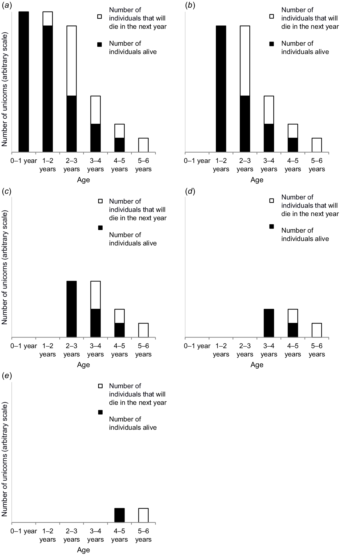
The black columns in Fig. 1 indicate the number of individuals of each age at any given time.
Given the above population characteristics, the total number of individuals in the population equals the sum of the black columns in Fig. 1a. These individuals can be considered as our study population at t = 0 years. In the following year, the original 0–1 year olds will be the new 1–2 year olds, and the number of these individuals that have died in this year is the white column in the 1–2 year old category. Similarly, the original 1–2 year olds will become the new 2–3 year olds, and the number of these individuals that have died in this year is the white column in the 2–3 year old category, and so on. By looking at Fig. 1a, it can be seen (without any mathematical equations) that the number of the original individuals that will die after a year (the total of the white columns) is equal to the number of the original population that were 0–1 year old.
Fig. 1b shows the study population at t = 1 year, and shows that the above method can be used to show that the number of the original unicorns that die after 2 years equals the number of the original individuals that were 1–2 years of age. At t = 1 year (Fig. 1b), none of our study population is now in the 0–1 year old category. As the population is stationary, the numbers of individuals in the other age categories are the same as in Fig. 1a). As previously, we can see that the number of 1–2 year olds that will die in the next year is the white column in the 2–3 year old column, the number of 2–3 year olds that will die in the next year is the white column in the 3–4 year old column, and so on. So, it can be seen (without any mathematical equations) that the number of the original unicorns that will die in the second year (the total of the white columns in Fig. 1b) is equal to the number of the original individuals that were 1–2 year olds.
The same process can be worked through in Fig. 1c–e to show that the number of unicorns that die in the third, fourth and fifth year is equal to the number in the stationary population that are 3–4, 3–4 and 4–5 years old.
Template for determining population age structure in wild populations
Fig. 1 demonstrates the relationship between population age structure and survivorship/mortality using charts of a stationary population with a known age structure. In a stationary population with unknown age structure but known survivorship, a chart illustrating survivorship from t = 0 years could be used to determine the number of individuals dying in each year, which would equate to the number of individuals in the corresponding age categories. By approaching the relationship from the starting point of survivorship, we can estimate population age structure from individuals of unknown ages.
We propose that with three broad assumptions, the age structure of a wild population can be determined by monitoring the survivorship of a sample of individuals from that population (‘sample survivorship’) – the proportion of individuals in each age category equating to the proportion of individuals that die in the corresponding period after the start of monitoring. The three assumptions are: (1) the population is stationary, (2) the age structure of individuals monitored is representative of the whole population, and (3) the survivorship of those individuals can be monitored accurately.
There are a number of other points to be noted in relation to the use of this method in a real-life setting. Firstly, Fig. 1 could be adjusted to show the same relationship for a population with any maximum age. Therefore, the derivation of population age structure can apply to a population whose maximum age is initially unknown. Equally, monitoring does not need to have reached the point of all the sample population being dead to know the proportion of individuals in the earlier age categories, and the proportion of individuals that remain alive at any time after the start of monitoring equals the proportion of individuals in the population that are older than that length of time.
Secondly, the method does not require any estimates of the ages of the sample individuals, nor does it give any information about the ages of the individuals. It just gives an estimate of the proportion of the individuals that are in each age category.
Lastly, it is likely that in many real-life situations there will be deviations to some degree from assumptions (1) and (2). In relation to assumption 1, while stationary populations are rare, it is common for populations to exhibit oscillations over time around an equilibrium structure, depending on external factors such as food availability, climate and disease (Bode and Possingham 2005). In relation to assumption 2, depending on the sample size, the sample may not be exactly representative of the whole population. Any such deviations from assumptions (which, it should be noted, are likely to affect any attempt to estimate population age structure) may lead to the observed proportions dying not exactly representing the actual proportions in the population age categories. For instance, in a period with an extreme weather event, the observed mortality rate may indicate a higher than real proportion of individuals in that age category; or in a period with favourable conditions, the observed mortality rate may indicate a lower than real proportion of individuals in that age category. Variations such as these may lead to the mortality rate in one period being higher than in the previous period. So simply using sample survivorship data to determine mortality rates and hence population age structure would lead to one age category in the population having a greater proportion of individuals than the previous age category (e.g. there being more 4-year-olds than 3-year-olds) – which is impossible in a stationary population. While the method we propose is unfamiliar to most with experience in wildlife survivorship and population age structure, we note that the issues described in this paragraph are likely to affect any attempt to estimate population age structure, even where it is possible to age individuals. As such, we suggest that to reject this method on the basis of these issues would miss the opportunity of providing important age structure estimates in populations where individual age cannot be accurately assessed. Instead, we propose that it would be appropriate to fit one or more regression line(s) through the sample survivorship data collected. More than one regression line should be fitted where the data suggest a different pattern of survivorship for different ages, consistent with the concept of stage based demography. Using this/these regression line(s), the mortality from one period to the next can then be calculated, and the estimated population age structure determined. Again, it is important to note that one age category cannot contain a greater proportion of the population than the previous age category. As such, when fitting the regression line(s), the rate of change of the survivorship curve can never increase.
Application to platypuses
Between August 2011 and August 2013, 154 platypuses (63 females > 1 year of age, three juvenile females, 82 males > 1 year of age, six juvenile males) were captured using fyke nets at 82 sites in the Inglis River catchment (41.06°S, 145.64°E) in north-west Tasmania. Each platypus was individually identified with a Trovan Unique® microchip inserted under the skin between the shoulder blades (Grant and Whittington 1991). Platypuses were classified as juvenile or older than 1 year of age by spur/spurs sheath morphology (Temple-Smith 1973; Williams et al. 2013; Macgregor 2015). Males were classified as juvenile if they had a full spur sheath present in the months January–June, or a full or partial spur sheath present July–December. Females were classified as juvenile if the spur sheath was retained in the months March–December. Additional confidence in these age assessments was provided by considering their body mass/size measurements (Macgregor 2015). Six sites were selected for ongoing survivorship remote monitoring using instream microchip antennas (Trovan®ANT 612, Trovan®ANT C600 and Trovan®ANT CUST) based on the land access and suitability of the water body for use of this technique (Macgregor et al. 2014). 2013 was selected as the starting point of the survivorship study. Platypuses were selected for the survivorship study if they were known to be alive in 2013, known to be at least 1 year old by spur/spur sheath morphology in 2013, and detected at any time at one or more of the six monitoring sites. This study group of 30 individuals consisted of four platypuses captured in 2011 and detected remotely at one of the study sites in 2013, 15 platypus captured in 2012 and detected remotely at one of the study sites in 2013, one platypus captured in 2012 and detected remotely at a study site in 2014, one platypus captured in 2012 and recaptured at a study site in 2015, and nine platypuses captured at the study sites in 2013.
Remote monitoring, and ongoing live capture/release fieldwork, was performed between 2014 and 2023. Sample survivorship data points were calculated for each of these years. Not all sites were monitored/trapped every year, dependent on the availability of resources within the project. To calculate each annual sample survivorship data point, only the platypuses from the sites monitored in that year were included. While some of the unmonitored individuals were known to be alive because they were observed in later years, the status of unmonitored individuals that were not subsequently detected was unknown. Any attempt to include data from any of these unmonitored individuals would introduce uncertainty and bias into the results. While the sample size used to create the sample survivorship data points varied between some of the years there is no reason to expect that any subset of the sample group of individuals is any less representative of the overall population. With the approach taken (excluding the possibility of migration of some individuals, which is addressed in the Discussion section) we can be confident of the status of each individual included in calculation of the sample survivorship data points, and so can be confident that each data point is valid.
A monitoring timeline was recorded by year from 2013 for each study individual. Each individual was recorded as ‘not alive’ in years when it was not detected by remote monitoring performed at the site(s) where it had been previously detected. The individual was recorded as ‘alive’ in years when it was detected by remote monitoring. In addition to this, any previous ‘not alive’ entries for this individual were changed to ‘alive’. With the exception of recaptures, no records were made for an individual in years when no remote monitoring was performed at its monitoring site. Recapture of an individual that occurred in a year when no remote monitoring occurred at that site was recorded as ’alive’ for that individual that year, and any previous ‘not alive’ entries were changed to ‘alive’. Because platypuses are known to avoid nets after initial capture (Griffiths et al. 2013), no entry was made in an individual’s monitoring timeline if it was not recaptured when trapping was performed.
The following assumptions in our methods should be made explicit, and will be explored in the Discussion. Firstly, we have assumed that any entry that remains as ‘not alive’ by the time of analysis denotes that the individual was dead in the year of the entry. Secondly, because not all sites were monitored each year, the number of individuals monitored each year was not the same. So, while the number of individuals monitored or alive may increase from one year to the next, on the assumption that ‘not alive’ equates to dead we consider that sample survivorship data point for each year is valid. Lastly, it should be noted again that when an ‘alive’ entry was made, previous ‘not alive’ entries were changed to ‘alive’, but years with no entries (indicating no monitoring at the relevant site) were left blank. As such, our sample survivorship data points below are calculated only from individuals whose sites were monitored and, again on the assumption that ‘not alive’ equates to dead, our sample survivorship data points remain valid.
Applying the above method to platypuses, for each year from 2014 to 2023 we calculated the proportion of individuals still alive (sample survivorship) as the number of individuals recorded as ‘alive’ divided by the sum of the number ‘alive’ and the number ‘not alive’. It was on these sample survivorship data points that subsequent analyses were performed. These yearly sample survivorship data points were calculated for female platypuses, male platypuses, and for the overall population.
Sample survivorship was plotted by year from the start of monitoring. The next step was to make a subjective decision as to whether any abrupt change in the distribution points was evident, to determine whether a single relationship should be sought for all the data points, or whether the data points should be grouped into more than one group of consecutive years for analysis.
To test whether there were sex differences in survival, we fit linear models to the proportion of animals that were known to be alive as the response variable, with year, sex, and the interaction between year and sex as predictors. We also compared models with polynomial and quadratic fit to the year, and tested variations of the model (for survival – 1) that forced the intercept through 0. We compared model rank using Akaike Information Criterion corrected for small sample size (AICc).
The formula for the best fit model was then used as our estimated cohort survivorship curve to determine the proportion of individuals expected to die during each period and hence the population age structure.
We made a crude assessment of the ability of our field methods to monitor individual survivorship by calculating the proportion of monitoring periods when detections were made for those platypuses that were known to be alive at the end of the study period, and then determining the average rate of non-detection for these individuals.
Results
The monitoring timelines for the 30 platypuses monitored are shown in Table 1. Table 2 shows the sample survivorship data. Fig. 2 illustrates the sample survivorship data by year over the course of the project and the derived population age structure. We made the subjective assessment that there were no clear changes in the distribution of the data points, so only one relationship between samples survivorship and time was sought.
 |
0, not detected at monitoring period or subsequently. 1, known to be alive at a monitoring period (by detection either at that monitoring period or subsequently). Bordered cells have had a 0 changed to a 1 by a subsequent detection. Shaded cells are recaptures. Empty cells indicate no monitoring was performed that year at the individual’s monitoring site. Horizontal lines group platypuses by monitoring site.
| Year | All | Female | Male | |||||||
|---|---|---|---|---|---|---|---|---|---|---|
| No. monitored | No. alive | % alive | No. monitored | No. alive | % alive | No. monitored | No. alive | % alive | ||
| 0 | 30 | 30 | 100 | 20 | 20 | 100 | 10 | 10 | 100 | |
| 1 | 10 | 9 | 90 | 6 | 5 | 83 | 4 | 4 | 100 | |
| 2 | 10 | 9 | 90 | 6 | 5 | 83 | 4 | 4 | 100 | |
| 3 | 10 | 8 | 80 | 6 | 5 | 83 | 4 | 3 | 75 | |
| 4 | 18 | 10 | 56 | 12 | 7 | 58 | 6 | 3 | 50 | |
| 5 | 17 | 10 | 59 | 12 | 8 | 67 | 5 | 2 | 40 | |
| 6 | 10 | 5 | 50 | 6 | 3 | 50 | 4 | 2 | 50 | |
| 7 | 14 | 7 | 50 | 8 | 3 | 38 | 6 | 4 | 67 | |
| 8 | 0 | 0 | 0 | |||||||
| 9 | 30 | 11 | 37 | 20 | 7 | 35 | 10 | 4 | 40 | |
| 10 | 30 | 8 | 27 | 20 | 5 | 25 | 10 | 3 | 30 | |
(a) Observed male and female sample survivorship by year with 95% confidence intervals around the regression lines. (b) Observed whole sample survivorship with the best model regression line (Proportion of cohort survivorship = −0.0755 × year + 1) and 95% confidence interval. (c) Derived age structure for the population.
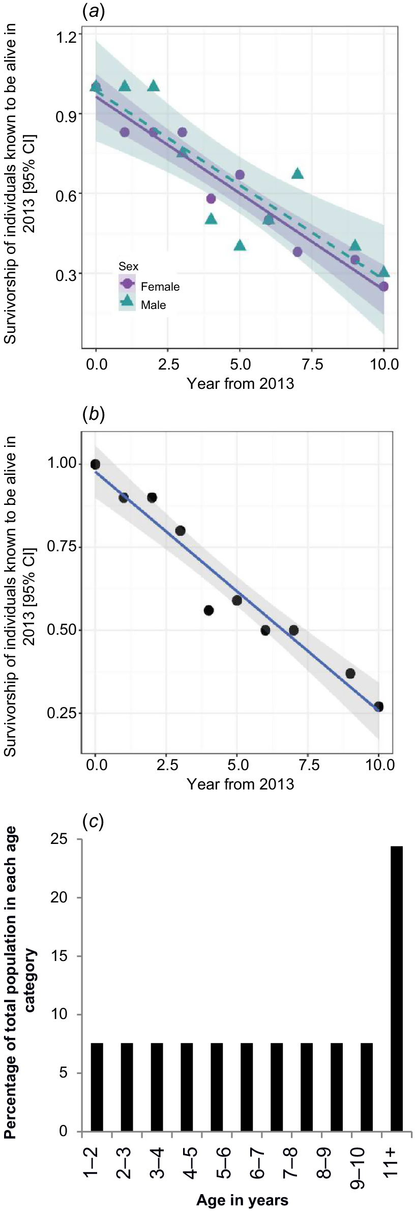
A single model describing survival was selected as having weight of support, with all other models having ΔAICc > 2 (Table 3). The best model included a linear fit to year and the intercept forced through zero (R2 = 0.946). The equivalent model that also included sex had a ΔAICc = 5.13; this result indicates that there was no weight of support for the assumption that there was difference in survival between males and females (Table 3, Fig. 2a). There was also no weight of support for the polynomial or quadratic line fits; therefore the linear fit was deemed the best fit to the data (Table 3).
| Model | d.f. | AICc | ΔAICc | R2 | |||
|---|---|---|---|---|---|---|---|
| m1 | m1 <- lm(Survival ~ Year × Sex, data = green) | 5 | −21.04 | 8.73 | 0.83823 | ||
| m2 | m2 <- lm(Survival ~ Year + Sex, data = green) | 4 | −24.65 | 5.13 | 0.83812 | ||
| m3 | m3 <- lm(Survival ~ Year, data = green) | 3 | −27.37 | 2.40 | 0.83448 | ||
| m4 | m4 <- lm(Survival ~ poly(Year,2) × Sex, data = green) | 7 | −15.21 | 14.56 | 0.86229 | ||
| m5 | m5 <- lm(Survival ~ poly(Year,2) + Sex, data = green) | 5 | −23.17 | 6.61 | 0.85453 | ||
| m6 | m6 <- lm(Survival ~ poly(Year,2), data = green) | 4 | −26.29 | 3.48 | 0.85090 | ||
| m7 | m7 <- lm(Survival ~ poly(Year,3) × Sex, data = green) | 9 | −2.86 | 26.91 | 0.86441 | ||
| m8 | m8 <- lm(Survival ~ poly(Year,3) + Sex, data = green) | 6 | −19.00 | 10.77 | 0.85461 | ||
| m9 | m9 <- lm(Survival ~ poly(Year,3), data = green) | 5 | −22.68 | 7.09 | 0.85098 | ||
| m1Z | m1Z <- lm((Survival-1) ~ Year × Sex + 0, data = green) | 5 | −21.04 | 8.73 | 0.94831 | ||
| m2Z | m2Z <- lm((Survival-1) ~ Year + Sex + 0, data = green) | 4 | −24.65 | 5.13 | 0.94828 | ||
| m3Z | m3Z <- lm((Survival-1) ~ Year + 0, data = green) | 2 | −29.77 | 0.00 | Best model | 0.94607 | |
| m4Z | m4Z <- lm((Survival-1) ~ poly(Year,2) × Sex + 0, data = green) | 7 | −15.21 | 14.56 | 0.95600 | ||
| m5Z | m5Z <- lm((Survival-1) ~ poly(Year,2) + Sex + 0, data = green) | 5 | −23.17 | 6.61 | 0.95352 | ||
| m6Z | m6Z <- lm((Survival-1) ~ poly(Year,2) + 0, data = green) | 3 | 25.08 | 54.85 | 0.27187 | ||
| m7Z | m7Z <- lm((Survival-1) ~ poly(Year,3) × Sex + 0, data = green) | 9 | −2.86 | 26.91 | 0.95668 | ||
| m8Z | m8Z <- lm((Survival-1) ~ poly(Year,3) + Sex + 0, data = green) | 6 | −19.00 | 10.77 | 0.95355 | ||
| m9Z | m9Z <- lm((Survival-1) ~ poly(Year,3) + 0, data = green) | 4 | 28.24 | 58.02 | 0.27190 | ||
The best fit relationship (Fig. 2b) produced the following estimated relationship for cohort survivorship between 1 and 11 years of age:
From this relationship, it is deduced that each age category from 1 to 11 years of age contains 7.55 ± 0.42 (s.e.) % of the total adult population, and platypuses over 11 years of age comprise 24.45% of the adult population (Fig. 2c). Of the eight platypuses known to be alive at the end of the study period, six were detected at every monitoring period, one was detected at 67% of monitoring periods and one was detected at 33% of monitoring periods. The average non-detection rate of these eight individuals was 12.5%.
Discussion
With our hypothetical illustration of a population of unicorns, this report provides a visual explanation of a previously described, but little-used, technique to investigate population age structure. The report then illustrates the application of this technique to a population of wild platypuses. Although our study is likely to have at least another decade to run, our interim results provide valuable baseline data for platypus population modelling, suggesting a population age structure/cohort survivorship that is markedly different from previously available data.
Applying the hypothetical method to a real-world population of platypuses in this study raises a number of issues that should be addressed. Firstly it may be suggested that stage-based demography is more useful than age-based demography (Caswell 2009). While this may be true in a range of species, it is not known if this is the case for the platypus and, to date, there is no method of differentiating adult platypuses into stages. Equally, even where stage-based demography is more appropriate, age and age-specific properties are still relevant to survivorship and longevity (Caswell 2009). As such, a population age structure is an important starting point from which further investigation of platypus demography, including whether stage based demography is an appropriate approach, can be performed.
Second, in any study involving analysis of rates of detection, detection probabilities should be discussed. Although not free from possible sources of bias, we consider that the mark–resight methods in this study provide meaningful results, and are a substantial improvement on studies relying on recapture with nets. While net avoidance has been observed in previously captured platypuses (Griffiths et al. 2013), and platypus recapture rates while currently unquantified are anecdotally known to be low, Macgregor et al. (2014) reported that in-stream antennas detected microchipped platypuses 93% of times they passed an antenna. The difference in detection rates is amplified by our antennas being in place for at least 2 weeks, as opposed to nets being in place for 1–4 days in most platypus capture field studies. As an example of the merits of in-stream antennas over recapture with nets, platypus 1 – detected by our in-stream antennas during all five monitoring periods at the site of her capture between 2013 and 2023 – wasn’t recaptured once during six nights of fieldwork that nets were in place at that site in the same period.
Migration of individuals away from the monitoring sites can decrease detections and therefore negatively bias survivorship data. However, we do not consider this to be a large source of bias. Despite having microchipped over 200 platypuses in the Inglis River Catchment, our remote monitoring and live capture work has detected only two movements of adults over 3 km (one of 11 km and one of 12 km) (Macgregor, unpubl. data) By contrast, juveniles have been observed to disperse over long distances (Serena and Williams 2013), and Bino et al. (2015) found recapture rates of juvenile platypuses to be significantly less than those of adults. Such juvenile dispersal could negatively bias repeat detection rates whether by in-stream antennas or repeat capture. As juvenile platypuses spend the first 4 months of their lives in their natal burrows (Grant 2007), a bias away from juveniles in the sample population is a further reason for their exclusion from this study. To combat these potential issues, we did not include juvenile platypuses, therefore avoiding the likely negative bias of juvenile dispersal.
Variability in detection probabilities between individuals is likely present; however, we make no comparisons between individuals. We assume that there is negative bias associated with our 2-week minimum monitoring period; constant monitoring would give the best possible results, but was not possible due to availability of resources, and access to monitoring sites. However, with a baseline 2-week monitoring period, if a monitoring period happened to run for longer than 2 weeks, any negative bias could only decrease. Although identical monitoring period lengths are ideal, small variations in the timing and duration of monitoring periods are common in wildlife fieldwork, and are one of the many uncertainties inherent in field research within which findings must be considered.
Although only a crude measure, our observation of an average non-detection rate of 12.5% in individuals that we know were alive at every monitoring period indicates that detection probability is likely to have a negative bias on our sample survivorship data. This bias is likely to be greater in the later years of monitoring, as opportunities to subsequently detect individuals and change a previous ‘not alive’ result back to ‘alive’ are reduced. This in turn is likely to result in a bias towards older individuals in the calculated population age structure and could explain why at least a small rate of mortality between 1 and 11 years was not observed. By continuing the monitoring for a number of years beyond when the last platypus is detected, we anticipate that this effect will be minimised in the final results.
The final issue to be considered in relation to the real-world application of the described method is whether the original sample population is representative of the whole population. This is an unknowable not unique to our study, but faced by all wildlife fieldwork.
Our results show a linear relationship between sample survivorship and year, and hence no evidence of high mortality between 1 and 11 years of age. This would be consistent with a type I or type III cohort survivorship curve (Deevey 1947), depending on mortality rates before and after 1–11 years of age. Monitoring platypuses from juveniles, Serena et al. (2014) show a steadily declining cohort survivorship curve for a population of platypuses in Victoria, consistent with a type II population. Unlike our results, they suggested that of the individuals alive at 2 years of age, only 24% remained alive 6 years later. These differences between the two studies could be explained by different population age structures. An alternative explanation for the apparent differences in survivorship curves/population age structures could be the differences between the methods. For example, avoidance of nets by previously captured platypuses (see above) would negatively bias redetection rates based on recapture. Equally, studies of the survivorship of juveniles are likely to be negatively biased by juvenile dispersal (see above). Use of the technique outlined in this paper for assessing survivorship in platypuses of all ages, rather than just juveniles, may be likely to reduce a negative bias associated with juvenile migration. With this hypothesis in mind, it would be interesting to apply this technique to the Serena et al. (2014) and Bino et al. (2015) datasets.
Bino et al. (2015) reported recapturing one female platypus over a 21 year period. This suggests that our survivorship study is at approximately its half-way point. Our linear cohort survival model, however, if extended into the future suggests a maximum age of between 14 and 15 years. The most likely explanation for this is that at some point in the future, the rate of change of our sample survivorship data will begin to decrease. This would be consistent both with a maximum life expectancy of over 15 years, as well as with a gradual decrease in cohort size/survivorship over several years rather than all individuals dying at around the same age. It seems likely that the mortality rates in older platypuses will be higher than in younger platypuses, consistent with the concept of stage based demography in which different life stages may exhibit different vital rates. If at some age there is a marked change in mortality rate, this may be visible in the subjective assessment of the data. In this situation, it may be considered appropriate to fit one regression line to the first years of data, and one or more to subsequent years.
Serena et al. (2014) reported higher maximum longevity estimates for male platypuses than females. By contrast, Bino et al. (2015) reported older maximum ages for females than males, and likewise observed survivorship was significantly higher for females than males. Although our data to date show no evidence of a difference in survivorship between males and females, continuation of the study is required to determine whether this changes over the age of 11 years.
The theory behind our method for using survivorship data to determine population age structure is not new; however, we hope we have brought it to the attention of researchers studying platypuses and other wildlife species. This method uses data from individuals of all, and unknown, ages. It avoids the need to either be able to accurately age individuals, or to have a large juvenile sample size. Although the precise way of monitoring survivorship is likely to vary between species and between studies, the availability of a method for determining population age structure from survivorship data may be valuable for the study, modelling, and management of a range of species for which individuals cannot be accurately aged.
Code of practice and research approvals
This study complied with the Australian Code for the Care and Use of Animals for Scientific Purposes. This study was approved by the Animal Ethics Committee of Murdoch University, Western Australia (Permit Numbers RW2422/11, RW2661/14, R3015/18 and RW3446/23), Department of Primary Industries, Parks, Water and Environment, Tasmania (Permit to take Wildlife for Scientific Purposes Numbers FA 11131, FA 12165, FA13937, FA14182, FA 15226, FA16252, FA17303, FA18081, FA20084, FA21049, FA22283 and FA23025) and Inland Fisheries Service, Tasmania (Exemption Permit Number 2011-10).
Data availability
A summary of the data used to generate the results in this paper is available in Table 1.
Declaration of funding
Financial support for this study was provided by a Holsworth Wildlife Research Endowment, Universities Federation for Animal Welfare Research Award and the Edward Alexander Weston and Iris Evelyn Fernie Research Fund.
References
Bino G, Grant TR, Kingsford RT (2015) Life history and dynamics of a platypus (Ornithorhynchus anatinus) population: four decades of mark–recapture surveys. Scientific Reports 5, 16073.
| Crossref | Google Scholar |
Bode M, Possingham H (2005) Optimally managing oscillating predator–prey systems. In ‘MODSIM 2005 International Congress on Modelling and Simulation’, December 2005. (Eds A Zerger, RM Argent) pp. 2054–2060. (Modelling and Simulation Society of Australia and New Zealand). Available at http://www.mssanz.org.au/modsim05/papers/%20Bode.pdf
Carey JR, Müller H-G, Wang J-L, Papadopoulos NT, Diamantidis A, Koulousis NA (2012) Graphical and demographic synopsis of the captive cohort method for estimating population age structure in the wild. Experimental Gerontology 47, 787-791.
| Crossref | Google Scholar | PubMed |
Caswell H (2009) Stage, age and individual stochasticity in demography. Oikos 118, 1763-1782.
| Crossref | Google Scholar |
Deevey ES, Jr. (1947) Life tables for natural populations of animals. The Quarterly Review of Biology 22, 283-314.
| Crossref | Google Scholar | PubMed |
Furlan E, Stoklosa J, Griffiths J, Gust N, Ellis R, Huggins RM, Weeks AR (2012) Small population size and extremely low levels of genetic diversity in island populations of the platypus, Ornithorhynchus anatinus. Ecology and Evolution 2, 844-857.
| Crossref | Google Scholar | PubMed |
Grant TR, Whittington RJ (1991) The use of freeze-branding and implanted transponder tags as a permanent marking method for the platypus, Ornithorhynchus anatinus (Monotremata: Ornithorhynchidae). Australian Mammalogy 14, 147-150.
| Crossref | Google Scholar |
Griffiths J, Kelly T, Weeks A (2013) Net-avoidance behaviour in platypuses. Australian Mammalogy 35, 245-247.
| Crossref | Google Scholar |
Macgregor JW, Holyoake CS, Munks S, Connolly JH, Robertson ID, Fleming PA, Warren KS (2014) Novel use of in-stream microchip readers to monitor wild platypuses. Pacific Conservation Biology 20, 376-384.
| Crossref | Google Scholar |
Mayne B, Mustin W, Baboolal V, Casella F, Ballorain K, Barret M, Vanderklift MA, Tucker AD, Korbie D, Jarman S, et al. (2022) Age prediction of green turtles with an epigenetic clock. Molecular Ecology Resources 22, 2275-2284.
| Crossref | Google Scholar | PubMed |
Müller H-G, Wang J-L, Carey JR, Caswell-Chen EP, Chen C, Papadopoulos N, Yao F (2004) Demographic window to aging in the wild: constructing life tables and estimating survival functions from marked individuals of unknown age. Aging Cell 3, 125-131.
| Crossref | Google Scholar | PubMed |
Parsons KM, Haghani A, Zoller JA, Lu AT, Fei Z, Ferguson SH, Garde E, Hanson MB, Emmons CK, Matkin CO, et al. (2023) DNA methylation-based biomarkers for ageing long-lived cetaceans. Molecular Ecology Resources 23, 1241-1256.
| Crossref | Google Scholar | PubMed |
Pelletier F, Moyes K, Clutton-Brock TH, Coulson T (2011) Decomposing variation in population growth into contributions from environment and phenotypes in an age-structured population. Proceedings of the Royal Society B: Biological Sciences 279, 394-401.
| Crossref | Google Scholar |
Rauschert E (2010) Survivorship curves. Nature Education Knowledge 3, 18.
| Google Scholar |
Serena M, Williams GA (2013) Movements and cumulative range size of the platypus (Ornithorhynchus anatinus) inferred from mark–recapture studies. Australian Journal of Zoology 60, 352-359.
| Crossref | Google Scholar |
Serena M, Williams GA, Weeks AR, Griffiths J (2014) Variation in platypus (Ornithorhynchus anatinus) life-history attributes and population trajectories in urban streams. Australian Journal of Zoology 62, 223-234.
| Crossref | Google Scholar |
Serena M, Snowball G, Thomas JL, Williams GA, Danger A (2024) Platypus longevity: a new record in the wild and information on captive life span. Australian Mammalogy 46(2), AM23048.
| Crossref | Google Scholar |
Vaupel JW (2009) Life lived and left: Carey’s equality. Demographic Research 20, 7-10.
| Crossref | Google Scholar |
Williams GA, Serena M, Grant TR (2013) Age-related change in spurs and spur sheaths of the platypus (Ornithorhynchus anatinus). Australian Mammalogy 35, 107-114.
| Crossref | Google Scholar |
Zhang Y, Bi J, Ning Y, Feng J (2024) Methodology advances in vertebrate age estimation. Animals 14, 343.
| Crossref | Google Scholar |