
Mesocarnivores in residential yards: influence of yard features on the occupancy, relative abundance, and overlap of coyotes, grey fox, and red fox
Emily P. Johansson A * and Brett A. DeGregorio B
A
B
Abstract
As conversion of natural areas to human development continues, there is a lack of information about how developed areas can sustainably support wildlife. While large predators are often extirpated from areas of human development, some medium-bodied mammalian predators (hereafter, mesocarnivores) have adapted to co-exist in human-dominated areas.
How human-dominated areas such as residential yards are used by mesocarnivores is not well understood. Our study aimed to identify yard and landscape features that influence occupancy, relative abundance and spatial-temporal overlap of three widespread mesocarnivores, namely, coyote (Canis latrans), grey fox (Urocyon cineroargenteus) and red fox (Vulpes vulpes).
Over the summers of 2021 and 2022, we deployed camera-traps in 46 and 96 residential yards, spanning from low-density rural areas (<1 home per km2) to more urban areas (589 homes per km2) in north-western Arkansas, USA.
We found that mesocarnivore occupancy was marginally influenced by yard-level features as opposed to landscape composition. Fences reduced the occupancy probability of coyotes, although they were positively associated with the total area of potential shelter sites in a yard. We found that relative abundance of grey fox was highest in yards with poultry, highlighting a likely source of conflict with homeowners. We found that all three species were primarily nocturnal and activity overlap between the species pairs was high.
Thus, these species may be using spatio-temporal partitioning to avoid antagonistic encounters and our data supported this, with few examples of species occurring in the same yards during the same 24-h period.
As the number of residential yards continues to grow, our results suggested that there are ways in which our yards can provide resources to mesocarnivores and that homeowners also have agency to mitigate overlap with mesocarnivores through management of their yard features.
Keywords: carnivores, mesocarnivores, occupancy, overlap, predators, residential yards, temporal activity patterns, yard features.
Introduction
Large mammalian predators and humans have a long and tumultuous history of struggling to co-exist (Fardell et al. 2020; Farr et al. 2022). However, as humans have altered the landscape to an unprecedented degree, mammalian mesocarnivores (medium-sized mammalian predators) such as coyote (Canis latrans) and foxes (Vulpes vulpes and Urocyon cinereoargenteus) often proliferate in human-dominated landscapes (Gehrt et al. 2011; Lombardi et al. 2017; Parsons et al. 2019). As human development expands, some bolder species are better able to occupy spaces within human-dominated areas than are others (Lombardi et al. 2017; Breck et al. 2019; Rodriguez et al. 2021). In these human-dominated areas, coyotes and foxes are often at the top of the food web and exert predatory pressure on deer, birds, and smaller mammals (Gompper 2002; Jones et al. 2016; Dyck et al. 2021). The presence of these species in and around human-dominated areas often draws extreme public interest in both positive and negative ways (Røskaft et al. 2007; Wilkinson 2023) and feelings can be the most extreme when these mesocarnivores are seen living in and around where humans reside (Farr et al. 2022).
One of the most prevalent human-dominated landcover types in North America is the suburban yard, which accounts for approximately 17.4% of the United States and covers more than 1.74 million km2 (Mathieu et al. 2007; Giner et al. 2013; Hedblom et al. 2017). Because homeowners use their yards for a variety of purposes, residential yards can be viewed as independently managed greenspaces that can vary widely in the resources that are of potential use to wildlife (Bolger et al. 2001; Gallo et al. 2017; Johansson and DeGregorio 2023). Although most yards are far smaller than the home range of mesocarnivores, they are frequently used by these species for foraging (Murray and St. Clair 2017), traveling (Noss et al. 2021), or denning (Way et al. 2001; Hansen et al. 2020; Raymond and St. Clair 2022) if the proper resources are present.
Mesocarnivores found in developed areas are often concentrated in green spaces such as parks and cemeteries (Parsons et al. 2019), but foray into residential areas to take advantage of subsidised resources (Prevedello et al. 2013) and can even shelter or raise young in residential yards (Way et al. 2001; Gosselink et al. 2003; Vuorisalo et al. 2014; Raymond and St. Clair 2022). Yards may be particularly attractive to mesocarnivores if they have dense populations of small mammal prey species owing to the presence of compost or refuse, bird feeders, pet food, or outdoor pets (Contesse et al. 2004; Timm et al. 2004; Newsome et al. 2014; Soulsbury and White 2015; Murray and St. Clair 2017; Hansen et al. 2020). Mesocarnivore diet can consist almost entirely of anthropogenic food sources (Contesse et al. 2004; Murray et al. 2015; Newsome et al. 2015; Reshamwala et al. 2018), including domestic pets and poultry (Larson et al. 2015). However, coyotes in urban environments may rely on natural prey items such as eastern cottontails (Sylvilagus floridanus) (Morey et al. 2007) and sometimes white-tailed deer (Newsome et al. 2015) and these prey species may preferentially reside in yards that contain features such as gardens. Additionally, infrastructure can provide safe and attractive denning or shelter opportunities under garages, decks, or outbuildings for both mesocarnivores and their prey species (Gosselink et al. 2003; Duduś et al. 2014). However, the suburban environment can also be heavily fragmented by fences separating yards, which can restrict access to yards. Coyotes and both fox species were less likely to be present in fenced yards (Hansen et al. 2020).
However, because yards are typically small, the features present in a yard may not be the only factors that influence where mesocarnivores occur. Wildlife often use habitat in a hierarchical fashion (Johnson 1980) and thus the composition of the surrounding landscape is almost certainly an important factor in mesocarnivore occupancy (Gehrt et al. 2009; Cooper et al. 2012). Residential yards situated in largely forested areas or surrounded by more open greenspace may be more likely to have mesocarnivores present, whereas they may be absent in yards surrounded by high-density housing or those surrounded primarily by impervious surface (roads, parking lots, buildings), even if the yards provide similar resources (Riley 1999; Riley et al. 2003; Kays et al. 2008; Morin et al. 2022).
Mesocarnivores living around humans often switch to being active primarily at night to avoid contact with humans and our dogs (Cove et al. 2012; Gese et al. 2012; Lowry et al. 2012; Gallo et al. 2017). However, if co-occurring mesocarnivore species concentrate their activity at night, they are more likely to have high activity overlap with one another (Moll et al. 2018; Gallo et al. 2022). This increase in overlap could possibly lead to antagonistic encounters among species (Gallo et al. 2022; Green et al. 2022). Thus, it is important to understand how these mesocarnivores alter their activity patterns in response to humans and if that increases temporal overlap among mesocarnivore species.
In the altered mammalian communities occurring around human development in the United States, coyotes, red and grey fox are often present and represent the largest carnivores (aside from black bears (Ursus americanus) and bobcats (Lynx rufus)) that regularly occur near people (Gehrt et al. 2009; Bateman and Fleming 2012; Lombardi et al. 2017). Red and grey foxes commonly occur in suburban environments and may even prefer these areas as opposed to more rural areas (Parsons et al. 2019; Hansen et al. 2020). Red foxes benefit by occurring in suburban areas because they can be protected from larger dominant carnivores such as coyotes and bobcats (Moll et al. 2018), a phenomenon referred to as the ‘human shield’ effect (Berger 2007). Even though coyotes are more cautious of residing in human-dominated areas than is red fox, they can also be regularly present throughout suburban and urban areas (Gehrt et al. 2011; Gil-Fernández et al. 2020). Grey foxes are not as common across developed areas; however, they often select denning sites near suburban development (Farías et al. 2012; Shannon et al. 2014; Moll et al. 2018; Sarkar and Bhadra 2022).
Our objectives were to use camera-traps to identify how yard features and surrounding landscape composition influence mesocarnivore occupancy, relative abundance (i.e. detection rate, which we defined as number of focal species detected per night), and interspecific temporal overlap in residential yards in a rapidly developing area. We predicted that mesocarnivore occupancy and relative abundance would be highest in yards with supplemental food and water such as compost piles, bird feeders, poultry, and garden ponds. Furthermore, we predicted that fences would decrease occupancy and relative abundance of all three species. We also predicted that both fox species would be less likely to occur in yards with coyote presence (Egan et al. 2021). We did not expect that the presence of one fox species would influence the occupancy of the other (Morin et al. 2022). Finally, we also predicted that as forest cover increases and housing-unit density decreases, coyote occupancy probability and relative abundance would increase (Riley 1999; Riley et al. 2003; Kays et al. 2008), whereas the opposite would be true for grey and red fox, which would most likely occur around developed open space (lawns, cemeteries, parks, golf courses etc.) (Moll et al. 2018). We also predicted that all mesocarnivore species would be primarily nocturnal and that the overlap of their activity patterns would thus be high.
Materials and methods
Study area
Our study was conducted in the north-western region of Arkansas, USA, which is a rapidly developing area with a population of approximately 350,000 people. Fayetteville is located within the Ozark Highlands Ecoregion, which is primarily forest intermixed with open areas and some pasture lands used for cattle and agriculture. Our study sites encompassed residential yards in and near the centres of Fayetteville, Springdale, Rogers, Eureka Springs, and Bella Vista and less developed areas up to 32 km from city centres (Fig. 1). The yards in which we conducted our study were owned by volunteers from the Arkansas Master Naturalist Program and University of Arkansas Department of Biological sciences. We restricted our study sites to yards occurring within an 80.5 km radius of downtown Fayetteville. We intentionally selected yards that represented a continuum of urban to rural setting as determined by surrounding housing-unit density (described below). We also ensured that we selected yards that contained (or did not contain) varying suites of a priori selected yard features associated with supplemental food, shelter, or water for wildlife (see below). Because volunteers came from the Master Naturalist Program and a Biology Department, not all yards contained features to attract wildlife and were representative of the yards available to wildlife in this region.
Map of study sites (residential yards) in north-western Arkansas, USA, during the summers of 2021 and 2022; study sites are indicated with a blue pin. (a) Large-scale view of the USA. (b) Finer-scale view of Arkansas, USA. (c) Finer-scale view of study sites within north-western region of Arkansas, USA.
Camera deployment
We deployed motion-triggered camera-traps (Browning StrikeForce or Spypoint ForceDark) in residential yards during the summers of 2021 and 2022. We deployed one camera per yard approximately 0.95 m above the ground on either a tripod or strapped to a tree. We placed cameras at least 5 m away from one another and no more than 100 m from a house. We positioned cameras to maximise wildlife detections, when possible, near features such as compost piles, water sources (natural or maintained), and fence lines or animal paths. We coordinated with homeowners to choose locations that would allow them to maintain their privacy and that also would not interfere with yard maintenance. If vegetation grew to impede the view of the camera, we would remove the vegetation. We set cameras to take a burst of three photos per trigger, with a 5 s reset time when triggered. We did not use any bait or lures at camera sites. Cameras were checked every 2 weeks to assess battery life and to download data. We moved cameras within yards up to three times within the season, to ensure that we captured the full range of wildlife present in each yard.
We surveyed each yard for features that we predicted would influence mesocarnivore occupancy (Table 1). We first recorded variables representing possible food sources, including the presence and number of bird feeders (both seed/suet and nectar), the volume of brush and firewood piles, area of compost piles, and the presence or absence of poultry. All area and volume calculations were undertaken by using a measuring tape to measure height, length, and width of the features. We reasoned that bird feeders could provide direct food to some of our focal species and could also serve as an attractant to prey species such as mice, rats, and birds (Saad et al. 2020). We considered the volume of firewood and brush piles as a food source because they could similarly be associated with high numbers of prey species (Goguen et al. 2015).
| Landscape covariate | Description of variable | Minimum | Maximum | Average | |
|---|---|---|---|---|---|
| Forest cover (NLCD) | Area of forest cover within 1.5 km buffer | 0.00 | 0.45 | 0.19 | |
| Open developed land (NLCD) | Area of open developed land, (parks, cemeteries, and lawns) within 1.5 km buffer | 0 | 0.31 | 0.09 | |
| Agricultural land (NLCD) | Area of land used for agricultural purposes within 1.5 km buffer | 0 | 0.43 | 0.09 | |
| Housing-unit density (HUD) (Radeloff et al. 2018) | Maximum HUD within 1.5 km buffer of camera (houses/km2) | 0.13 | 5094.60 | 589.41 | |
| Developed land (high + medium intensity) (NLCD) | Area of land that with greater than 49% impervious surface within 1.5 km buffer | 0 | 0.23 | 0.04 | |
| Developed land (low intensity) (NLCD) | Area of land that contains between 20% and 49% impervious surface within 1.5 km buffer | 0 | 0.30 | 0.08 | |
| Environmental covariates | |||||
| Average temperature (NOAA) | Average temperature over a 7-day period (°C) | 2021: 14.72 2022: 13.89 | 2021: 28 2022: 29.67 | 2021: 26.04 2022: 24.42 | |
| Average precipitation (NOAA) | Average precipitation over a 7-day survey period (cm.) | 2021: 0 2022: 0 | 2021: 1.45 2022: 6.25 | 2021: 0.43 2022: 1.50 | |
| Yard-feature covariates | |||||
| Volume of denning sites | Volume under sheds/outbuildings and under decks less than 1 m off the ground (m3) | 0 | 700 | 24.35 | |
| Volume of brush piles | Volume of brush piles (m3) | 0 | 335.94 | 38.65 | |
| Volume of firewood | Volume of firewood piles (m3) | 0 | 13 | 0.72 | |
| Supplemental water source | Number of human-maintained water sources | 0 | 7 | 0.85 | |
| Compost pile | Area of compost pile (m2) | 0 | 16 | 0.40 | |
| Fence type | If a camera was within a fence, it was given a score of either zero or one, zero being a fence that is permeable to most wildlife and one being the most impassable. | 18 yards had fences, 85 did not | |||
| Poultry presence | Presence or absence of poultry being kept in yard | 97 yards did not have poultry, 9 did | |||
| Bird feeders | Number of bird feeders at a camera site, including seed feeders, suet, hummingbird feeders, and dried fruit. | 0 | 19 | 3.15 | |
| Year | Year that the yard was surveyed | NA | NA | NA | |
We also recorded the area of potential sheltering sites in a yard. Sheltering sites included the total available area of sheds and outbuildings under which animals could access as well as decking that was less than 0.3 m off the ground (Linduska 1947; Moll et al. 2018). We counted the number of supplemental water sources present in a yard, which included bird baths, garden ponds, and fountains that were actively maintained by the homeowner.
If a camera was deployed in an area that was surrounded by a fence, we scored the type of fence based on its ease of access to our focal species. We scored each yard with a binary score of zero or one. Yards without fences or with fences that presented minimal resistance to the movement of our focal species (barbed wire or those made of semi spaced slats 1 m tall that allowed for smaller-bodied species to pass through and most larger species to jump over) were given a zero. If a fence was fallen, had large holes in them, or had a gate that was always left open, the fence also received a score of zero. Privacy and chain-link fences that were 1.8 m or taller and were made of a solid material, that were likely to prevent the passage of focal species, apart from capable climbers, were given a one.
Landscape and environmental covariates
To acquire landscape-level covariates to explain mesocarnivore occupancy and relative abundance, we calculated the area of several landcover types surrounding each focal yard. First, we imported all camera-location points to GIS (ArcGIS Pro 10.2; ESRI, Inc. Redlands Inc.) and created 1.5 km buffers around each camera on the basis of a reasonable approximation of mesocarnivore home ranges (Šálek et al. 2015). Within each buffer, we then calculated the area of forest cover, developed open land (e.g. cemeteries, parks, and grass lawns), and agricultural land (grasslands, cultivated crops, and pastureland) by using the 2019 National Land Cover Database (Dewitz and US Geological Survey 2021). We used two different development categories for analyses because we predicted that our focal species might respond differently to development of varying intensities. We used low-intensity development, which was represented by areas containing 20–49% of impervious surface. We then grouped the National Land Cover Database (NLCD) categories of medium- and high-intensity development (which we refer to as high intensity development) that contained areas with over 49% impervious surface. We also quantified the maximum housing-unit density (HUD) around each camera by using the SILVIS Housing Data Layer (Radeloff et al. 2018).
Mesocarnivore occupancy
To explore the effects of covariates on the detection and occupancy of our three focal mesocarnivores (coyotes, red and grey foxes), we used a single-season multi-species occupancy model (MacKenzie et al. 2002). Our occupancy models were used to estimate the probability that a mesocarnivore occurred in a yard and the influence of covariates on occupancy probability while accounting for imperfect detection (MacKenzie et al. 2004). We chose multispecies models to account for avoidance or attraction between our focal species. Multispecies occupancy allowed us to simultaneously model environmental covariates, while letting the occupancy of one species vary on the basis of the presence of another. We used individual yards as our survey locations and within each survey location, we used 1-week sampling periods. For each sampling period, we assigned a one or a zero for each species at each survey location. If the focal species was detected during a survey period at a site, a one was assigned, and if none was detected, a zero was assigned. We used a 1-week sampling period because this represented an appropriate amount of time as to not over- or under-compress statistical power and is consistent with numerous occupancy analyses conducted using camera-traps (Trolle and Kéry 2003; MacDougall and Sander 2022). During the summer of 2022, we resampled 41 of our study yards from 2021. For these sites, we created year–site combinations and treated them as independent sites, as in previous studies (Hines et al. 2014; Devenish-Nelson and Nelson 2021; Murray et al. 2021). We used year as an occupancy covariate (Linden and Roloff 2013) to explore whether patterns differed between the 2 years of the study. Not all cameras in yards were actively functioning for the duration of the entire season because of camera malfunctions or staggered deployment and pick-up dates. To correct for this, we censored weeks in which the camera was not operating continuously for all 7 days. We censored these camera weeks by assigning a ‘NA’ value as opposed to a one or a zero.
We also compiled a number of environmental covariates that we predicted would influence the behaviour or activity of our three focal species. Both rainfall and temperature can influence how active our species were and therefore could affect detection probability (Madsen et al. 2020). We defined detection probability as the chance that a species would be detected on a given day. To gather environmental variables, we used publicly available data from a National Oceanic and Atmospheric Association (NOAA) weather station located at the Fayetteville Experimental Station. This weather station was 75 km from the furthest yard studied. We used this data to calculate the average weekly air temperature and average weekly precipitation for each camera site.
Before model fitting, we assessed collinearity of covariates and considered any two covariates to be collinear if they had correlation coefficients ≥|0.6| (Gilhooly et al. 2019). From those, we would then decide which of the two variables were predicted to be more meaningful and only included that variable in subsequent analyses (Gilhooly et al. 2019). For detection covariates in occupancy analyses, we found that temperature was correlated with both precipitation (r = −0.61) and week of the survey (r = 0.72) and was therefore subsequently removed. When assessing occupancy covariates, high-intensity development was correlated with area of low intensity development (r = 0.75) as well as forested area (r = −0.74). Area of low development was also found to be correlated with forested areas (r = 0.73). Both development levels were subsequently removed from analyses. So as to facilitate comparison between variables measured on different scales, we centered all continuous covariates by subtracting the variable mean value and then dividing by one standard deviation (Schielzeth 2010).
To avoid model over-fitting, we used a multi-stage fitting approach (Fuller et al. 2016) to select for the best detection covariate. We modelled mean precipitation, week of the year, an additive model of week + precipitation, and a null model as covariates for detection against null occupancy parameters and selected the top covariate model using Akaike’s information criterion corrected for small sample size (AICc). The covariate(s) in the top model were then used as the detection covariates in all subsequent analyses of occupancy probability.
For occupancy covariates, we included the area of compost pile, supplemental water sources, poultry presence, number of bird feeders, fence type, as well as the volumes of denning sites, firewood piles, and brush piles (Table 1). We also included four landscape-level occupancy covariates, including the areas of open development, agriculture, forest, and HUD.
Our candidate model set included all possible two-way additive combinations of occupancy covariates with our top identified detection covariate(s) as well as a global and a null model. All model fitting was performed in R (R Core Team 2022, available at https://www.r-project.org/) with the unmarked package (Fiske and Chandler 2011, available at https://cran.r-project.org/web/packages/unmarked/index.html). To improve clarity in presenting model selection tables, we display only models that were competitive within two ΔAICc. Because there was model uncertainty, we used full model averaging (Lukacs et al. 2009) for all the model estimates to generate an average of unconditional occupancy estimates (Cade 2015).
Mesocarnivore relative abundance
In addition to mesocarnivore occupancy, we also examined how yard and landcover covariates influenced the relative abundance of each focal species. We defined relative abundance as the number of focal species detections at each site (yard) divided by the total number of trap-nights. Although this metric often correlates with true abundance (Campbell et al. 2015), it is more often used as an index of intensity of use within an area and thus could be a good complement to occupancy, which is a coarser metric (Martin et al. 2010). Because camera-traps take multiple photographs at once, we combined all photos taken within a 5 min period into one ‘detection’ to minimise double-counting of individuals. To evaluate which landcover and yard variables most influenced the relative abundance of our mesocarnivore species in each yard, we used a generalised linear model (GLM) analysis. We used separate GLM analyses for each species to explore how landscape and yard features affected how frequently a mesocarnivore was detected in a yard. For each analysis, we evaluated the same candidate models as those used in the occupancy analyses. The candidate model set for each analysis consisted of simple one-way variable models and all additive two-way combinations as well as a global and a null model.
For each analysis, we ranked candidate models by using an information-theoretic approach with AICc. When appropriate, we derived parameter estimates for candidate models by model averaging all models within two ΔAICc (Burnham and Anderson 2002) in R (R Core Team 2022) with the AICcmodavg package (R package version 2.3.2, available at https://cran.rproject.org/package=AICcmodavg).
To improve clarity in presenting model selection tables, we display only models that were competitive within two ΔAICc for each analysis. Initial exploratory analyses indicated that relationships between predictor variables and response variables were linear and thus models were not corrected. Full model averaging was used to avoid bias away from zero (Lukacs et al. 2009). Model goodness-of-fit was assessed using residual plots and examining the R2 value (R2 = 0.12).
Interspecific temporal overlap
To better understand interspecific temporal overlap, we calculated the activity overlap between each species pair by using the R package overlap (Meredith and Ridout 2021; available at https://cran.r-project.org/web/packages/overlap/index.html). We created kernels of activity for each species to quantify when during the diel period they were most active. We first converted the time that each species was detected to radians. We then calculated a species-specific non-parametric kernel around the detection times to quantify when each species was active. For each species pair, we calculated the overlapped area under the kernel curve for the species pair. This number was quantified along a 0–1 index, with zero representing no overlap and one representing complete overlap (Schmid and Schmidt 2006). For our purposes, we used the Δ4 value (a vector of densities estimated at the time of observation) because we had over 75 detections of each species (Schmid and Schmidt 2006; Ridout and Linkie 2009). We used detections from across all of our study sites collectively to create activity kernels.
To assess the time between interspecific detections, we calculated the time elapsed between detections of one species in a yard and the next chronological detection of the next focal species in the same yard. We first did this by days between, and then for anything with less than 24 h between detections, we calculated hours between the detections.
Results
Over the course of two seasons, we surveyed 138 yards across north-western Arkansas. During the 2021 season, we deployed cameras in 46 yards between 1 May and 10 August and surveyed these sites for up to 15 weeks (mean ± s.d., 14 ± 1.5). In 2022, we deployed cameras at 92 yards between 1 May and 10 August and surveyed these yards for up to 15 weeks (mean ± s.d., 14 ± 2.5).
Mesocarnivore occupancy
Cumulatively, we conducted 1456 week-long surveys for a total of 10,192 trap-nights and accumulated 1,494 focal mesocarnivore detections (507 coyote, 157 grey fox, and 830 red fox). We detected at least one mesocarnivore (coyote, grey fox, or red fox) in 74% of yards. Two species were present at 25 yards, whereas only six yards had all three species present.
Coyotes were detected at 51% of yards during 191 survey periods, grey fox at 14% of yards in 52 surveys, and red fox at 40% of yards during 160 surveys. The occupancy probability (ψ) for at least one mesocarnivore in a yard was 0.74 (95% credibility interval (CI): 0.66–0.80). The ψ of coyotes was 0.54 (95% CI: 0.43–0.63), ψ of grey fox 0.14 (95% CI: 0.09–0.26), and ψ of red fox was 0.41 (95% CI: 0.31–0.53). The detection probability (pi) was similar among the three species, with pi of coyotes averaging 0.18 (95% CI: 0.16–0.22), pi of grey fox averaging 0.19 (95% CI: 0.14–0.25), and pi of red fox averaging 0.20(95% CI: 0.17–0.24). Preliminary modelling for detection covariates suggested that the best predictors for mesocarnivore detection at a yard were the additive effect of week and average precipitation, and this model accounted for 63% of the weight of evidence (Table 2). Coyotes and red fox were less likely to be detected later in the summer and coyotes and grey fox were more likely to be detected during rainy weeks. Therefore, we used week and average precipitation as the pi covariates for all analyses of ψ.
| Model | K | AICc | ΔAICc | AICcWt | LL | |
|---|---|---|---|---|---|---|
| Ψ(.), p(week + rain) | 15 | 2492.04 | 0.00 | 0.63 | −1229.07 | |
| Ψ(.), p(week) | 12 | 2493.30 | 1.26 | 0.34 | −1233.41 |
Covariates of detection included week of the survey and average weekly precipitation. Models were ranked using Akaike’s information criterion corrected for small sample size (AICc) and included with each model is the number of parameters (K), AICc difference between model of interest and model with lowest AICc (ΔAICc), model weight (AICcwt) and log-likelihood estimate (LL).
The three candidate models predicting mesocarnivore occupancy that were within 2 ΔAICc units of one another all assumed pairwise dependence between species. These top models accounted for 36% of the weight of evidence (Table 3). Two of the top models included fence type, one of which also included compost piles in the model; however, credibility intervals overlapped for all species for effect of compost pile. The other model that received some weight of evidence was the area of shelter sites (Table 3 and Supplementary material Table S1). Fences reduced coyote ψ (β = −0.92, 95% CI: −0.93, −0.07) but coyote ψ increased when sheltering area was abundant (β = 0.01, 95% CI:0.00, 0.01) (Fig. 2). We found no evidence that any of the measured covariates influenced ψ of red or grey fox (Table 4).
| Model | K | AICc | ΔAICc | AICcWt | LL | |
|---|---|---|---|---|---|---|
| Ψ(fence), p(precipitation + week) | 18 | 0.00 | 0.00 | 0.17 | −1225.85 | |
| Ψ(fence × compost), p(precipitation + week) | 18 | 1.12 | 1.12 | 0.10 | −1226.41 | |
| Ψ(den site), p(precipitation + week) | 18 | 1.35 | 1.35 | 0.09 | −1226.53 |
95% credibility intervals for covariates from our top a priori models evaluating detection (pi) and occupancy probability (ψ) of coyote (Canis latrans), grey fox (Urocyon cinereoargenteus), and red fox (Vulpes vulpes) occurring in residential yards during the summers of 2021 and 2022 in north-western Arkansas, USA.
| Species | Model | ψ(fence) | ψ(compost) | ψ(shelter site) | p(rain) | p(week) | |
|---|---|---|---|---|---|---|---|
| Coyote | Ψ(fence), p(rain + week) | −0.92 (95% CI = −0.93, −0.07) | – | – | 0.43 (95% CI = 0.05, 0.82) | −0.05 (95% CI = −0.09, −0.01) | |
| Ψ(fence + compost), p(rain + week) | −0.50 (95% CI = −0.93, −0.07) | −0.08 (95% CI = −0.37, 0.21) | – | 0.43 (95% CI = 0.05, 0.82) | −0.05 (95% CI = −0.09, −0.01) | ||
| Ψ(shelter site), p(rain + week) | – | – | 0.01 (0.00,0.01) | 0.44 (95% CI = 0.05, 0.81) | −0.05 (95% CI = −0.09, −0.01) | ||
| Grey fox | Ψ(fence), p(rain + week) | −0.20 (95% CI = −0.82, 0.42) | – | – | 0.83 (95% CI = 0.03, 1.61) | −0.05 (95% CI = −0.12, 0.02) | |
| Ψ(fence + compost), p(rain + week) | −0.18 (95% CI = −0.80, 0.43) | 0.15 (95% CI = −0.15, 0.47) | – | 0.82 (95% CI = 0.03, 1.61) | −0.05 (95% CI = −0.12,0.02) | ||
| Ψ(shelter site), p(rain + week) | – | – | −0.01 (−0.03, 0.01) | 0.82 (95% CI = 0.03, 1.61) | −0.05 (95% CI = −0.12, 0.02) | ||
| Red fox | Ψ(fence), p(rain + week) | −0.07 (95% CI = −0.31, 0.45) | – | – | 0.06 (95% CI = −0.39,0.51) | −0.05 (95% CI = −0.09, −0.01) | |
| Ψ(fence + compost), p(rain + week) | −0.06 (95% CI = −0.32, 0.45) | −0.35 (95% CI = −0.79, 0.08) | – | 0.06 (95% CI = −0.39,0.50) | −0.05 (95% CI = −0.09, −0.01) | ||
| Ψ(shelter site), p(rain + week) | – | – | 0.00 (>0.00,0.00) | 0.06 (95% CI = −0.39,0.50) | −0.05 (95% CI = −0.09, −0.01) |
We found that Ψ of all our study species increased if another species was also present in that yard (Table 5). This relationship was strongest for coyote, given that a red fox was present, with grey fox having the weakest influence from coyote presence.
| Species interaction | Conditional occupancy | |
|---|---|---|
| Coyote × grey fox | 0.55 | |
| Coyote × red fox | 0.58 | |
| Grey fox × coyote | 0.15 | |
| Grey fox × red Fox | 0.17 | |
| Red fox × coyote | 0.45 | |
| Red fox × grey fox | 0.50 |
Relative abundance
We found little evidence for the effects of covariates influencing the relative abundance of coyote or red fox in a yard and the null model was the top-ranked model for both species. We found two top models for grey fox relative abundance within two ΔAICc that accounted for 42% of the weight of evidence (Table 6). Both top models included poultry presence and the top model also included forested area (Table 6). These models suggest that relative abundance of grey fox was highest in yards with a chicken coop (model-averaged β = 0.06, 95% CI: 0.01–0.3) (Fig. 3).
| Model | K | AICc | ΔAICc | AICcWt | LL | |
|---|---|---|---|---|---|---|
| Poultry presence + forest | 4.00 | −445.66 | 0.00 | 0.27 | 226.98 | |
| Poultry presence | 3.00 | −444.44 | 1.22 | 0.15 | 225.31 |
Species temporal overlap
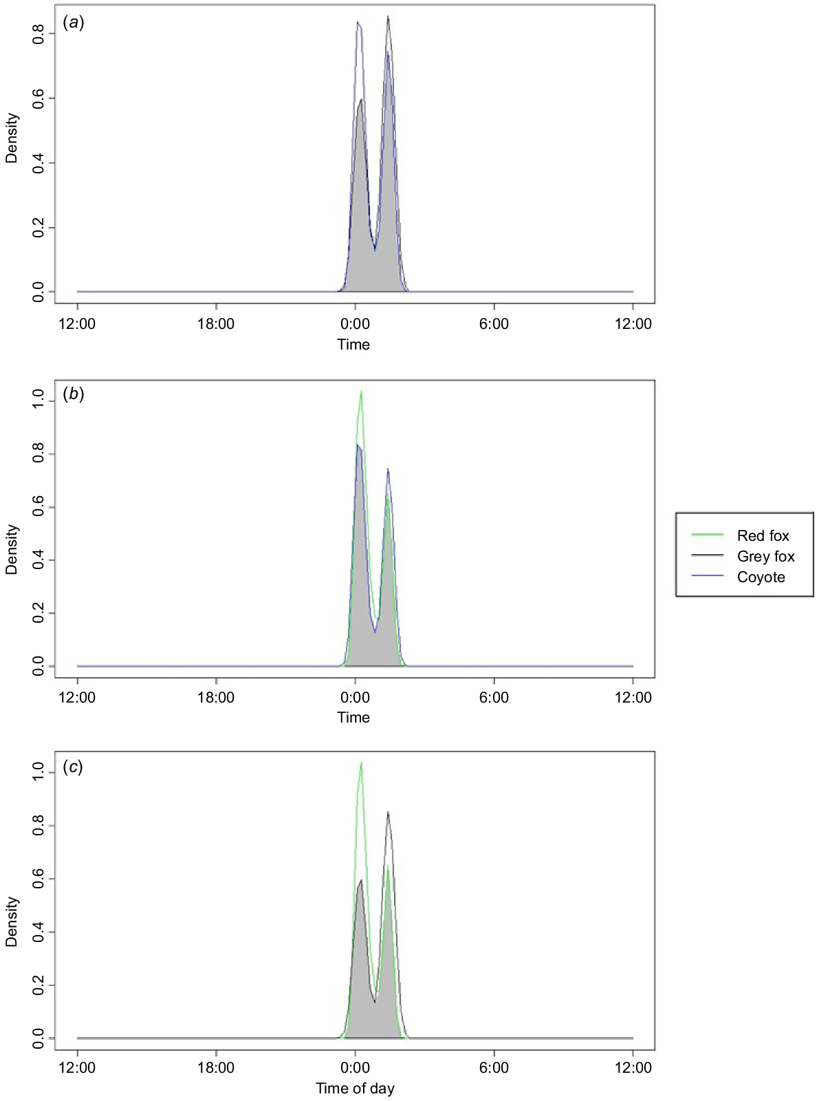
When assessing the activity times of our focal species, we found that they were all predominantly nocturnal. All species had peak activity levels approximately at midnight. Coyotes and grey fox had an 87.8% temporal overlap (95% CI: 79.0–95.3) (Fig. 4) and coyotes and red fox had an 89.6% temporal overlap (95% CI: 84.7–94.4) (Fig. 4). Grey and red fox had a temporal overlap of 78.1% (95% CI: 68.5–87.0) (Fig. 4).
Kernel temporal overlap between species across all sites within a 2-year study conducted in 2021 and 2022 in residential yards in north-western Arkansas, USA. (a) Grey fox (Urocyon cinereoargenteus) and coyote (Canis latrans). (b) Red fox (Vulpes vulpes) and coyote (Canis latrans). (c) Grey fox (Urocyon cinereoargenteus) and red fox (Vulpes vulpes).
Most of our focal mesocarnivores were not detected during the same night in the same yards. For example, grey fox and coyote detections were, on average, 4 (±5.5 s.d.) days apart (min: 0; max: 22). Coyote and red fox had the longest separation between detections, with an average of 12 (±19) days (min: 0; max: 88). Grey fox and red fox were separated by an average of 7 days (±4.4) days (min: 0; max: 33). If the species were detected within the same 24-h period, we calculated the average time between detections and found that coyote and grey fox had an average of 11 (±9.7) h between detections (min: 0.4; max: 23.5) at nine sites where they were both detected within the same 24-h period. Coyotes and red fox had an average of 7.6 (±7.6) h between detections at 15 sites (min: 0.96; max: 22). Red and grey fox were detected within the same 24-h period at only two sites and were detected an average of 14 (±5.9) h apart (min: 10.14; max: 18.5).
Discussion
Contrary to our predictions, food resources provided by homeowners in residential yards were not the top factors explaining patterns in occupancy for coyote, red fox, or grey fox. However, we did find evidence that the relative abundance of grey fox was highest in yards with chickens, although our top model also included forested area. Curiously, Kays and Parsons (2014) and Hansen et al. (2020) did not find an association between grey fox and chicken coops. Previous studies have shown that these and other mesocarnivores are attracted to yards on the basis of food resources such as compost piles and bird feeders (Murray et al. 2015; Hansen et al. 2020; Saad et al. 2020). We had expected to find a stronger effect because many mesocarnivores found in suburban areas have been shown to have diets consisting of human-subsidised food items (Bateman and Fleming 2012; Murray et al. 2015; Hansen et al. 2020).
We also predicted that shelter availability would influence occupancy and relative abundance of our focal species. Red foxes have frequently been documented denning and sheltering in suburban habitats (Gosselink et al. 2003; Vuorisalo et al. 2014). There is also evidence that coyotes can shelter in residential yards (Way et al. 2001; Grubbs and Krausman 2009; Raymond and St Clair 2022). However, we found only modest evidence that coyote occupancy increased in yards with abundant shelter opportunities and no evidence that red fox or grey fox occupancy or relative abundance was influenced by shelter availability in yards. This finding is surprising, given the well-documented history of red fox denning in yards as well as observations during this study of red fox denning in some of the study yards. Not only do red foxes frequently shelter in residential yards, but they prey on smaller species that are likely to be attracted to sheltering sites, such as groundhog (Marmota monax), eastern cottontails (Sylvilagus floridanus) etc. (Linduska 1947; Goguen et al. 2015; Moll et al. 2018).
Our study found compelling evidence that fences can be used to keep coyotes out of yards. Although coyotes have some ability to climb fences (Thompson 1979), it is unlikely that they can or are willing to climb all fence types. It appears that they spend less time in fenced yards than in unfenced yards. Hansen et al. (2020) also found that fences were a deterrent to larger mammalian species in yards (Hansen et al. 2020). This is a positive outcome for homeowners unwilling to share their space with coyotes (Baker and Timm 1998). However, in some areas of the United States, 86% of suburban lawns are fenced (Ossola et al. 2019; Van Helden et al. 2020), which is likely to create fragmentation and barriers to wildlife species such as the coyote.
Our study had several shortcomings that may have contributed to the lack of support for our predictions. We found no support for landscape variables influencing patterns of occupancy or relative abundance and believe that this may be due to the fact that our study area was largely forested. Perhaps a study conducted in a more heterogeneous landscape may find different results. It is also possible that evaluating our data on a different scale or multiple spatial scales could lead to different inferences (McGarigal et al 2016). Finally, our selection of yards might not have been truly representative of the spectrum of available wildlife resources. Although we attempted to choose yards representing the full range of available resources, the majority of our volunteers were from the Arkansas Master Naturalists, a demographic that may be more prone to feeding birds, gardening for wildlife, and providing natural resources than is the public at large.
Although our species can be flexible in their activity, we found that they were overwhelmingly nocturnal in residential yards, having peak activity times from 23:00 hours to 3:00 hours (Fig. 4). This condensing of activity time is most likely to be due to an avoidance of human activity (Gaynor et al. 2018; Gallo et al. 2022; Green et al. 2022; Mims et al. 2022). Because these species are pushed to all be active at the same time in the suburban environment, and our results suggest that they choose yards for similar reasons (Fig. 4) (Larson et al. 2015), they are likely to be using a form of spatio-temporal partitioning to avoid using the same yards during the same days (Gosselink et al. 2003; Mueller et al. 2018). This is supported as detections of multiple species in the same yard were spread out by numerous days. Our study found it relatively rare to detect multiple mesocarnivores in a yard within less than 24 h, having only 16 yards in which this occured. We found that our species were detected an average of 11 days apart. Other studies also showed that when these species overlap in territory (i.e. a yard), foxes tend to shift when and where they are active to avoid encountering coyotes (Moll et al. 2018; Mueller et al. 2018; Cervantes et al. 2023).
Our study is a representation of how three mesocarnivore species use residential yards in north-western Arkansas. We found that at least one of our focal species (coyote) was detected in 74% of our surveyed residential yards. Because the number of suburban residential yards continues to grow across the country, the factors that bring mesocarnivores to yards and how to mitigate the conflicts that will likely arise (Bolger et al. 2001; Hansen et al. 2020) are areas for future research. Although large mesocarnivores often face public persecution, they continue to persist in suburban areas despite fear of them and widespread negative public perception (Bonnell and Breck 2016). Homeowners do have some agency in how they manage their yards and how these resources either attract or deter mesocarnivores.
Declaration of funding
Funding for this project was provided by the University of Arkansas Office of Undergraduate Research, the Arkansas Game and Fish Commission via cooperative agreement Number 1434-04HQRU1567, and the National Science Foundation through support for the Research Experience for Undergraduates program.
Acknowledgements
This project would not have been possible without our generous and incredible volunteers from the Department of Biological Sciences at the University of Arkansas, and the Arkansas State Master Naturalists. Any use of trade, firm, or product names is for descriptive purposes only and does not imply endorsement by the US Government. This paper forms part of the MS thesis of Emily Johansson (2023).
References
Baker RO, Timm RM (1998) Management of conflicts between urban coyotes and humans in southern California. In ‘Proceedings of the Vertebrate Pest Conference. Vol. 18’. (University of California) Available at https://doi.org/10.5070/v418110164
Bateman PW, Fleming PA (2012) Big city life: carnivores in urban environments. Journal of Zoology 287(1), 1-23.
| Crossref | Google Scholar |
Berger J (2007) Fear, human shields and the redistribution of prey and predators in protected areas. Biology Letters 3(6), 620-623.
| Crossref | Google Scholar | PubMed |
Bolger DT, Scott TA, Rotenberry JT (2001) Use of corridor-like landscape structures by bird and small mammal species. Biological Conservation 102(2), 213-224.
| Crossref | Google Scholar |
Bonnell MA, Breck S (2016) Using coyote hazing at the community level to change coyote behavior and reduce human-coyote conflict in urban environments. In ‘Proceedings of the Vertebrate Pest Conference. Vol. 27’. (University of California) Available at https://doi.org/10.5070/v427110354
Breck SW, Poessel SA, Mahoney P, Young JK (2019) The intrepid urban coyote: a comparison of bold and exploratory behavior in coyotes from urban and rural environments. Scientific Reports 9(1), 2104.
| Crossref | Google Scholar |
Burnham KP, Anderson DR (2002) ‘Model selection and inference: a practical information-theoretic approach.’ 2nd edn. (Springer-Verlag: New York) Available at https://doi.org/10.1007/b97636
Cade BS (2015) Model averaging and muddled multimodel inferences. Ecology 96, 2370-2382.
| Crossref | Google Scholar | PubMed |
Campbell MD, Pollack AG, Gledhill CT, Switzer TS, DeVries DA (2015) Comparison of relative abundance indices calculated from two methods of generating video count data. Fisheries Research 170, 125-133.
| Crossref | Google Scholar |
Cervantes AM, Schooley RL, Lehrer EW, Gallo T, Allen ML, Fidino M, Magle SB (2023) Carnivore coexistence in Chicago: niche partitioning of coyotes and red foxes. Urban Ecosystems 26(5), 1293-1307.
| Crossref | Google Scholar |
Contesse P, Hegglin D, Gloor S, Bontadina F, Deplazes P (2004) The diet of urban foxes (Vulpes vulpes) and the availability of anthropogenic food in the city of Zurich, Switzerland. Mammalian Biology 69(2), 81-95.
| Crossref | Google Scholar |
Cooper SE, Nielsen CK, McDonald PT (2012) Landscape factors affecting relative abundance of gray foxes Urocyon cinereoargenteus at large scales in Illinois, USA. Wildlife Biology 18(4), 366-373.
| Crossref | Google Scholar |
Cove MV, Jones BM, Bossert AJ, Clever DR, Jr, Dunwoody RK, White BC, Jackson VL (2012) Use of camera traps to examine the mesopredator release hypothesis in a fragmented Midwestern landscape. The American Midland Naturalist 168(2), 456-465.
| Crossref | Google Scholar |
Devenish-Nelson ES, Nelson HP (2021) Abundance and density estimates of landbirds on Grenada. Journal of Caribbean Ornithology 34, 88-98.
| Crossref | Google Scholar |
Dewitz J, US Geological Survey (2021) National Land Cover Database (NLCD) 2019 products (ver. 2.0, June 2021): US Geological Survey data release. Available at https://doi.org/10.5066/P9KZCM54
Duduś L, Zalewski A, Kozioł O, Jakubiec Z, Król N (2014) Habitat selection by two predators in an urban area: the stone marten and red fox in Wrocław (SW Poland). Mammalian Biology 79(1), 71-76.
| Crossref | Google Scholar |
Dyck MA, Wyza E, Popescu VD (2021) When carnivores collide: a review of studies exploring the competitive interactions between bobcats Lynx rufus and coyotes Canis latrans. Mammal Review 52(1), 52-66.
| Crossref | Google Scholar |
Egan ME, Day CC, Katzner TE, Zollner PA (2021) Relative abundance of coyotes (Canis latrans) influences gray fox (Urocyon cinereoargenteus) occupancy across the eastern United States. Canadian Journal of Zoology 99(2), 63-72.
| Crossref | Google Scholar |
Fardell LL, Pavey CR, Dickman CR (2020) Fear and stressing in predator–prey ecology: considering the twin stressors of predators and people on mammals. PeerJ 8, e9104.
| Crossref | Google Scholar |
Farías V, Fuller TK, Sauvajot RM (2012) Activity and distribution of gray foxes (Urocyon cinereoargenteus) in southern California. The Southwestern Naturalist 57(2), 176-181.
| Crossref | Google Scholar |
Farr JJ, Pruden MJ, Glover R, Murray MH, Sugden SA, Harshaw HW, Cassady St. Clair C (2022) A ten-year community reporting database reveals rising coyote boldness and associated human concern in Edmonton, Canada. Ecology and Society 28(2),.
| Crossref | Google Scholar |
Fiske I, Chandler R (2011) unmarked: an R package for fitting hierarchical models of wildlife occurrence and abundance. Journal of Statistical Software 43(10), 1-23.
| Crossref | Google Scholar |
Fuller AK, Linden DW, Royle JA (2016) Management decision making for fisher populations informed by occupancy modeling. Journal of Wildlife Management 80(5), 794-802.
| Crossref | Google Scholar |
Gallo T, Fidino M, Lehrer EW, Magle SB (2017) Mammal diversity and metacommunity dynamics in urban green spaces: implications for urban wildlife conservation. Ecological Applications 27(8), 2330-2341.
| Crossref | Google Scholar | PubMed |
Gallo T, Fidino M, Gerber B, Ahlers AA, Angstmann JL, Amaya M, Drake D, Gay D, Lehrer EW, Murray MH, Ryan TJ, Cassady St Clair C, Salsbury CM, Sander HA, Stankowich T, Williamson J, Belaire JA, Simon K, Magle SB (2022) Mammals adjust diel activity across gradients of urbanization. eLife 11, e74756.
| Crossref | Google Scholar | PubMed |
Gaynor KM, Hojnowski CE, Carter NH, Brashares JS (2018) The influence of human disturbance on wildlife nocturnality. Science 360(6394), 1232-1235.
| Crossref | Google Scholar | PubMed |
Gehrt SD, Anchor C, White LA (2009) Home range and landscape use of coyotes in a metropolitan landscape: conflict or coexistence? Journal of Mammalogy 90(5), 1045-1057.
| Crossref | Google Scholar |
Gehrt SD, Brown JL, Anchor C (2011) Is the urban coyote a misanthropic synanthrope? The case from Chicago. Cities and the Environment 4(1), 1-25.
| Crossref | Google Scholar |
Gil-Fernández M, Harcourt R, Newsome T, Towerton A, Carthey A (2020) Adaptations of the red fox (Vulpes vulpes) to urban environments in Sydney, Australia. Journal of Urban Ecology 6(1), juaa009.
| Crossref | Google Scholar |
Gilhooly PS, Nielsen SE, Whittington J, St. Clair CC (2019) Wildlife mortality on roads and railways following highway mitigation. Ecosphere 10(2), e02597.
| Crossref | Google Scholar |
Giner NM, Polsky C, Pontius RG, Jr, Runfola DM (2013) Understanding the social determinants of lawn landscapes: a fine-resolution spatial statistical analysis in suburban Boston, Massachusetts, USA. Landscape and Urban Planning 111, 25-33.
| Crossref | Google Scholar |
Goguen CB, Fritsky RS, San Julian GJ (2015) Effects of brush piles on small mammal abundance and survival in central Pennsylvania. Journal of Fish and Wildlife Management 6, 392-404.
| Crossref | Google Scholar |
Gompper ME (2002) Top carnivores in the suburbs? ecological and conservation issues raised by colonization of north eastern North America by coyotes. BioScience 52(2), 185.
| Crossref | Google Scholar |
Gosselink TE, Deelen TRV, Warner RE, Joselyn MG (2003) Temporal habitat partitioning and spatial use of coyotes and red foxes in east-central Illinois. The Journal of Wildlife Management 67(1), 90.
| Crossref | Google Scholar |
Green AM, Barnick KA, Pendergast ME, Şekercioğlu ÇH (2022) Species differences in temporal response to urbanization alters predator–prey and human overlap in northern Utah. Global Ecology and Conservation 36, e02127.
| Crossref | Google Scholar |
Grubbs SE, Krausman PR (2009) Use of urban landscape by coyotes. The Southwestern Naturalist 54(1), 1-12.
| Crossref | Google Scholar |
Hansen CP, Parsons AW, Kays R, Millspaugh JJ (2020) Does use of backyard resources explain the abundance of urban wildlife? Frontiers in Ecology and Evolution 8, 570771.
| Crossref | Google Scholar |
Hedblom M, Lindberg F, Vogel E, Wissman J, Ahrné K (2017) Estimating urban lawn cover in space and time: case studies in three Swedish cities. Urban Ecosystems 20(5), 1109-1119.
| Crossref | Google Scholar |
Hines JE, Nichols JD, Collazo JA (2014) Multiseason occupancy models for correlated replicate surveys. Methods in Ecology and Evolution 5(6), 583-591.
| Crossref | Google Scholar |
Johansson EP, DeGregorio BA (2023) Effects of landscape cover and yard features on feral and free-roaming cat (Felis catus) distribution, abundance and activity patterns in a suburban area. Journal of Urban Ecology 9(1), juad003.
| Crossref | Google Scholar |
Johnson DH (1980) The comparison of usage and availability measurements for evaluating resource preference. Ecology 61(1), 65-71.
| Crossref | Google Scholar |
Jones BM, Cove MV, Lashley MA, Jackson VL (2016) Do coyotes Canis latrans influence occupancy of prey in suburban forest fragments? Current Zoology 62(1), 1-6.
| Crossref | Google Scholar | PubMed |
Kays R, Parsons AW (2014) Mammals in and around suburban yards, and the attraction of chicken coops. Urban Ecosystems 17(3), 691-705.
| Crossref | Google Scholar |
Kays RW, Gompper ME, Ray JC (2008) Landscape ecology of eastern coyotes based on large-scale estimates of abundance. Ecological Applications 18(4), 1014-1027.
| Crossref | Google Scholar | PubMed |
Larson RN, Morin DJ, Wierzbowska IA, Crooks KR (2015) Food habits of coyotes, gray foxes, and bobcats in a coastal southern California urban landscape. Western North American Naturalist 75(3), 339-347.
| Crossref | Google Scholar |
Linden DW, Roloff GJ (2013) Retained structures and bird communities in clearcut forests of the Pacific Northwest, USA. Forest Ecology and Management 310, 1045-1056.
| Crossref | Google Scholar |
Linduska JP (1947) Winter den studies of the cottontail in southern Michigan. Ecology 28(4), 448-454.
| Crossref | Google Scholar |
Lombardi JV, Comer CE, Scognamillo DG, Conway WC (2017) Coyote, fox, and bobcat response to anthropogenic and natural landscape features in a small urban area. Urban Ecosystems 20(6), 1239-1248.
| Crossref | Google Scholar |
Lowry H, Lill A, Wong BBM (2012) Behavioural responses of wildlife to urban environments. Biological Reviews 88, 537-549.
| Crossref | Google Scholar | PubMed |
Lukacs PM, Burnham KP, Anderson DR (2009) Model selection bias and Freedman’s paradox. Annals of the Institute of Statistical Mathematics 62(1), 117-125.
| Crossref | Google Scholar |
MacDougall B, Sander H (2022) Mesopredator occupancy patterns in a small city in an intensively agricultural region. Urban Ecosystems 25(4), 1231-1245.
| Crossref | Google Scholar |
MacKenzie DI, Nichols JD, Lachman GB, Droege S, Andrew Royle J, Langtimm CA (2002) Estimating site occupancy rates when detection probabilities are less than one. Ecology 83, 2248-2255.
| Crossref | Google Scholar |
MacKenzie DI, Bailey LL, Nichols JD (2004) Investigating species co-occurrence patterns when species are detected imperfectly. Journal of Animal Ecology 73(3), 546-555.
| Crossref | Google Scholar |
Madsen AE, Corral L, Fontaine JJ (2020) Weather and exposure period affect coyote detection at camera traps. Wildlife Society Bulletin 44(2), 342-350.
| Crossref | Google Scholar |
Martin J, Chamaillé-Jammes S, Nichols JD, Fritz H, Hines JE, Fonnesbeck CJ, MacKenzie DI, Bailey LL (2010) Simultaneous modeling of habitat suitability, occupancy, and relative abundance: African elephants in Zimbabwe. Ecological Applications 20(4), 1173-1182.
| Crossref | Google Scholar | PubMed |
Mathieu R, Freeman C, Aryal J (2007) Mapping private gardens in urban areas using object-oriented techniques and very high-resolution satellite imagery. Landscape and Urban Planning 81(3), 179-192.
| Crossref | Google Scholar |
McGarigal K, Wan HY, Zeller KA, Timm BC, Cushman SA (2016) Multi-scale habitat selection modeling: a review and outlook. Landscape Ecology 31(6), 1161-1175.
| Crossref | Google Scholar |
Meredith M, Ridout M (2021) Estimates of coefficient of overlapping for animal activity patterns. Available at https://cran.r-project.org/web/packages/overlap/overlap.pdf [Accessed 9 May 2022]
Mims DM, Yasuda SA, Jordan MJ (2022) Contrasting activity times between raccoons (Procyon lotor) and Virginia opossums (Didelphis virginiana) in urban green spaces. Northwestern Naturalist 103(1), 63-75.
| Crossref | Google Scholar |
Moll RJ, Cepek JD, Lorch PD, Dennis PM, Robison T, Millspaugh JJ, Montgomery RA (2018) Humans and urban development mediate the sympatry of competing carnivores. Urban Ecosystems 21(4), 765-778.
| Crossref | Google Scholar |
Morey PS, Gese EM, Gehrt S (2007) Spatial and temporal variation in the diet of coyotes in the Chicago metropolitan area. The American Midland Naturalist 158(1), 147-161.
| Crossref | Google Scholar |
Morin DJ, Lesmeister DB, Nielsen CK, Schauber EM (2022) Asymmetrical intraguild interactions with coyotes, red foxes, and domestic dogs may contribute to competitive exclusion of declining gray foxes. Ecology and Evolution 12(7), e9074.
| Crossref | Google Scholar |
Mueller MA, Drake D, Allen ML (2018) Coexistence of coyotes (Canis latrans) and red foxes (Vulpes vulpes) in an urban landscape. PLoS ONE 13(1), e0190971.
| Crossref | Google Scholar |
Murray MH, St. Clair CC (2017) Predictable features attract urban coyotes to residential yards. The Journal of Wildlife Management 81(4), 593-600.
| Crossref | Google Scholar |
Murray M, Cembrowski A, Latham ADM, Lukasik VM, Pruss S, St Clair CC (2015) Greater consumption of protein-poor anthropogenic food by urban relative to rural coyotes increases diet breadth and potential for human–wildlife conflict. Ecography 38(12), 1235-1242.
| Crossref | Google Scholar |
Murray MH, Fidino M, Lehrer EW, Simonis JL, Magle SB (2021) A multi-state occupancy model to non-invasively monitor visible signs of wildlife health with camera traps that accounts for image quality. Journal of Animal Ecology 90(8), 1973-1984.
| Crossref | Google Scholar | PubMed |
Newsome TM, Ballard G-A, Fleming PJS, van de Ven R, Story GL, Dickman CR (2014) Human-resource subsidies alter the dietary preferences of a mammalian top predator. Oecologia 175(1), 139-150.
| Crossref | Google Scholar | PubMed |
Newsome SD, Garbe HM, Wilson EC, Gehrt SD (2015) Individual variation in anthropogenic resource use in an urban carnivore. Oecologia 178(1), 115-128.
| Crossref | Google Scholar | PubMed |
Noss RF, Cartwright JM, Estes D, Witsell T, Elliott G, Adams D, Albrecht M, Boyles R, Comer P, Doffitt C, Faber-Langendoen D, Hill JV, Hunter WC, Knapp WM, Marshall ME, Singhurst J, Tracey C, Walck J, Weakley A (2021) Improving species status assessments under the US Endangered Species Act and implications for multispecies conservation challenges worldwide. Conservation Biology 35(6), 1715-1724.
| Crossref | Google Scholar | PubMed |
Ossola A, Locke D, Lin B, Minor E (2019) Greening in style: urban form, architecture and the structure of front and backyard vegetation. Landscape and Urban Planning 185, 141-157.
| Crossref | Google Scholar |
Parsons AW, Rota CT, Forrester T, Baker-Whatton MC, McShea WJ, Schuttler SG, Millspaugh JJ, Kays R (2019) Urbanization focuses carnivore activity in remaining natural habitats, increasing species interactions. Journal of Applied Ecology 56(8), 1894-1904.
| Crossref | Google Scholar |
Prevedello JA, Dickman CR, Vieira MV, Vieira EM (2013) Population responses of small mammals to food supply and predators: a global meta-analysis. Journal of Animal Ecology 82(5), 927-936.
| Crossref | Google Scholar | PubMed |
R Core Team (2022) R: A Language and Environment for Statistical Computing. R Foundation for Statistical Computing, Vienna, Austria. Available at https://www.r-project.org/
Radeloff VC, Helmers DP, Kramer HA, Mockrin MH, Alexandre PM, Bar-Massada A, Butsic V, Hawbaker TJ, Martinuzzi S, Syphard AD, Stewart SI (2018) Rapid growth of the US wildland–urban interface raises wildfire risk. Proceedings of the National Academy of Sciences 115(13), 3314-3319.
| Crossref | Google Scholar |
Raymond S, St. Clair CC (2022) Urban coyotes select cryptic den sites near human development where conflict rates increase. The Journal of Wildlife Management 87(1), e22323.
| Crossref | Google Scholar |
Reshamwala HS, Shrotriya S, Bora B, Lyngdoh S, Dirzo R, Habib B (2018) Anthropogenic food subsidies change the pattern of red fox diet and occurrence across Trans-Himalayas, India. Journal of Arid Environments 150, 15-20.
| Crossref | Google Scholar |
Ridout MS, Linkie M (2009) Estimating overlap of daily activity patterns from camera trap data. Journal of Agricultural, Biological, and Environmental Statistics 14(3), 322-337.
| Crossref | Google Scholar |
Riley SPD, Sauvajot RM, Fuller TK, York EC, Kamradt DA, Bromley C, Wayne RK (2003) Effects of urbanization and habitat fragmentation on bobcats and coyotes in southern California. Conservation Biology 17(2), 566-576.
| Crossref | Google Scholar |
Rodriguez JT, Lesmeister DB, Levi T (2021) Mesocarnivore landscape use along a gradient of urban, rural, and forest cover. PeerJ 9, e11083.
| Crossref | Google Scholar |
Røskaft E, Händel B, Bjerke T, Kaltenborn BP (2007) Human attitudes towards large carnivores in Norway. Wildlife Biology 13(2), 172-185.
| Crossref | Google Scholar |
Saad SM, Sanderson R, Robertson P, Lambert M (2020) Effects of supplementary feed for game birds on activity of brown rats Rattus norvegicus on arable farms. Mammal Research 66(1), 163-171.
| Crossref | Google Scholar |
Šálek M, Drahníková L, Tkadlec E (2015) Changes in home range sizes and population densities of carnivore species along the natural to urban habitat gradient. Mammal Review 45, 1-14.
| Crossref | Google Scholar |
Sarkar R, Bhadra A (2022) How do animals navigate the urban jungle? A review of cognition in urban-adapted animals. Current Opinion in Behavioral Sciences 46, 101177.
| Crossref | Google Scholar |
Schielzeth H (2010) Simple means to improve the interpretability of regression coefficients. Methods in Ecology and Evolution 1(2), 103-113.
| Crossref | Google Scholar |
Schmid F, Schmidt A (2006) Nonparametric estimation of the coefficient of overlapping—theory and empirical application. Computational Statistics & Data Analysis 50(6), 1583-1596.
| Crossref | Google Scholar |
Shannon G, Angeloni LM, Wittemyer G, Fristrup KM, Crooks KR (2014) Road traffic noise modifies behaviour of a keystone species. Animal Behaviour 94, 135-141.
| Crossref | Google Scholar |
Soulsbury CD, White PCL (2015) Human–wildlife interactions in urban areas: a review of conflicts, benefits and opportunities. Wildlife Research 42(7), 541-553.
| Crossref | Google Scholar |
Thompson BC (1979) Evaluation of wire fences for coyote control. Journal of Range Management 32(6), 457-461.
| Crossref | Google Scholar |
Timm RM, Baker RO, Bennett JR, Coolahan CC (2004) Coyote attacks: an increasing suburban problem. UC Davis: Hopland Research and Extension Center. Available at https://escholarship.org/uc/item/8qg662fb
Trolle M, Kéry M (2003) Estimation of ocelot density in the Pantanal using capture–recapture analysis of camera-trapping data. Journal of Mammalogy 84(2), 607-614.
| Crossref | Google Scholar |
Van Helden BE, Close PG, Steven R (2020) Mammal conservation in a changing world: can urban gardens play a role? Urban Ecosystems 23(3), 555-567.
| Crossref | Google Scholar |
Vuorisalo T, Talvitie K, Kauhala K, Bläuer A, Lahtinen R (2014) Urban red foxes (Vulpes vulpes L.) in Finland: a historical perspective. Landscape and Urban Planning 124, 109-117.
| Crossref | Google Scholar |
Way JG, Auger PJ, Ortega IM, Strauss EG (2001) Eastern coyote denning behavior in an anthropogenic environment. Northeast Wildlife 56, 18-30.
| Google Scholar |
Wilkinson CE (2023) Public interest in individual study animals can bolster wildlife conservation. Nature Ecology & Evolution 7, 478-479.
| Crossref | Google Scholar |