

An experiential account with recommendations for the design, installation, operation and maintenance of a farm-scale soil moisture sensing and mapping system
Brendan Malone A * , David Biggins B , Chris Sharman B , Ross Searle C , Mark Glover A and Stuart Brown D
A
B
C
D
Abstract
The research explores the benefits of real time tracking of soil moisture for various land management contexts and the importance of spatio-temporal modelling and mapping to gain clear and visual understanding of soil moisture fluxes across a farm.
This research aims to outline the key processes required for building an operational on-farm soil moisture monitoring system where the product is highly granular daily soil moisture maps depicting variations temporally, spatially and vertically.
We describe processes of capacitance soil moisture probe installation, data collection infrastructure, sensor calibration, spatio-temporal modelling, and mapping.
An out-of-bag soil moisture evaluation modelling system was tested for nearly 2 years. We found a model accuracy (RMSE) estimate of 0.002 cm−3 cm−3 and concordance of 0.96 were found. This result is averaged over this period but fluctuated daily, and related to rainfall patterns across the target farm, which were not directly incorporated into the modelling framework. As expected, incorporating prior estimates of soil moisture into the modelling framework contributed to very accurate estimates of real time available soil moisture.
This research promotes the importance of iterative improvements to the soil moisture monitoring system, particularly in areas of sensor recalibration and spatio-temporal modelling. We stress the need for a longer-term view and plan for ongoing maintenance and improvement of such systems in the emerging digital farming ecosystem.
The results of this research will be useful for researchers and practitioners involved in the design and implementation of on-farm soil monitoring systems.
Keywords: agriculture, digital agriculture, digital soil mapping, generalised additive models, IoT, sensor calibration, soil modelling, soil moisture, soil moisture sensing, soil monitoring.
Introduction
Soil moisture is a critical factor for the existence of agriculture, and therefore has played a vital role in the development and sustainability of human civilisation. In addition to its role in agriculture, soil moisture plays a critical role in the water cycle, and the global climate system (McColl et al. 2017). Soil moisture affects the exchange of water and energy between land surface and atmosphere, which have implications for regional and global climate patterns. Soil moisture also affects the risk of flooding, bushfires and erosion, as well as the transport of water and sediments in watersheds.
A diverse array of methods can be used for measurement of soil moisture, ranging from direct gravimetric approaches (McKenzie et al. 2002), tensiometers (Richards and Gardner 1936), electrical resistivity sensors (Kean et al. 1987), neutron probes (Visvalingam and Tandy 1972), electromagnetic induction (Rhoades et al. 1976; Huth and Poulton 2007), capacitance (Campbell 1990) and time domain reflectometry (TDR; Dalton and Van Genuchten 1986) sensors, and infra-red spectroscopy (Blaschek et al. 2019). The viability of each of these approaches depends on the specific needs of the user, including the accuracy required, the frequency of monitoring, the cost, the required expertise, and resourcing to carry out these different approaches.
With the emergence of ‘smart farming’, the Internet of Things (IoT), and the related digital convergence (Wadoux and McBratney 2021), the integration of the cyber and physical components of farm management and agribusiness operations is increasingly entwined. For farming contexts, granular monitoring of soil moisture provides an agribusiness manager a precision capability to manage crop productivity.
Despite the growing use of sensor-based soil moisture monitoring at farm-scales, there are fragmented efforts regarding the technical aspects of the establishment, operation, data curation and analytics that underpin and support a successful program of farm-based soil moisture monitoring. Our aim in this experiential-based research is to resolve this fragmentation by outlining these processes, with the aim to provide guidance for establishing and maintaining an on-farm soil moisture sensing system.
The benefits of sensor-based soil moisture monitoring support many on-farm decisions like time of planting, nutrient management, harvest options such as growing a crop out for grain, or grazing it with livestock, baling it for hay or making silage. With timely soil moisture information, in-crop marketing strategies for the previously mentioned product options are available, facilitating greater marketing diversity and forward-selling opportunities. Where irrigation is actively practiced, precision scheduling can also be enabled. But from an agricultural resilience and adaptation perspective, such networks could provide insights into early warning signs for the detection of drought conditions and their subsequent monitoring (Jung et al. 2020). Similarly with changing climates, a much-observed phenomenon across agricultural zones across the world, changes in precipitation patterns, temperature and evaporation rates can significantly impact available soil moisture, and being able to quickly quantify these changes enables more adaptable agricultural practices. For soil science and vadose zone research, soil water monitoring and granular insights of soil moisture provides better information to drive research into nutrient fluxes and biogeochemical cycling more broadly.
Systems of inter-connected soil moisture sensors (soil moisture sensor networks, SMSN) address issues of single point of measurements to enable better spatial characterisation (Brown et al. 2023). These networks typically consist of several sensors placed at different locations and depths across some prescribed spatial extent (field, farm, catchment etc.), which are connected to a data logger or some other data acquisition system. The most common types of sensors deployed in a SMSN are based on capacitance measurement or TDR measurement techniques (Bogena et al. 2022). The sensors measure soil moisture at regular intervals, and the data transmitted wirelessly or through a wired connection to a computer or server. Compared with remote sensing of soil moisture, SMSNs enable unmatched ability to measure and monitor soil moisture at depth, in and beyond the root zone, and potentially with higher granularity.
While our study is limited to in-field installations of soil moisture sensors, remote sensing of soil moisture (Petropoulos et al. 2015) is also an emerging science. Although limited to measurement of the soil surface currently, together with other operational and scale (for highly granular characterisation) challenges, the abilities to characterise soil moisture across large spatial extents via remote sensing enhances monitoring capabilities of this critical resource.
In this research, we describe the deployment of 36 soil moisture probes across a 290-ha farm in southern New South Wales, Australia. A description of the hardware and supporting data infrastructure is provided for background, but it is acknowledged the choices around equipment selection, data logging processes and density of sensors are a matter for the owner and operator of the SMSN and the contexts for which they are established. Moreover, we describe the logic of sensor placement, as the need to deploy them in such a way to maximise spatial and environment coverage is critical to deriving sensible inferences of the spatial and temporal variability of soil moisture fluxes. We then describe the processes of soil-specific calibration (Gasch et al. 2017), followed by integration of sensor information with a data-rich digital soil informatic system (Malone et al. 2022) that extends soil moisture readings from the probe scale to highly granular model daily predictions across a farm. We also highlight that SMSNs are not set-and-forget systems. From regular equipment maintenance and monitoring to modular-based improvements of supporting data analytics, keeping such systems running over long time scales requires ongoing dedicated expertise and resources.
Materials and methods
Methodological overview
A general stepwise process of establishing an on-farm soil monitoring system entails:
Selection of the type and quantity of soil moisture probes.
Provision of a data collection and analytics system to collect and store data streams that would be measured by the soil moisture probes.
Installation of soil moisture probes and establish connection with data collection system.
Integrate into analytics system, processes for sensor calibration and re-calibration to return site specific measures of available soil moisture.
Further integration of system to take output from Step 4 into a spatio-temporal modelling framework to output maps at an established granularity and time step.
Revisit Steps 4 and 5 periodically seeking to improve processes with the intention of gaining more accuracy.
Routine monitoring of the integrity of probes in the field and data collected by them.
A lot of the work described in this research is centred around Steps 4 and 5. Steps 1–3 describe the specific context of the farm where this research was conducted. Step 6 is not included in the methodological work of this research, but rather processes of its implementation is described in the discussion part of the manuscript.
The site
Boorowa Agricultural Research Station (BARS) is a 290-ha mixed cropping farming enterprise situated in south-eastern New South Wales, Australia. It is located 3 km south of the town of Boorowa (34.4386S, 148.7231S) in the Boorowa River catchment located within the Lachlan Fold Belt. The terrain ranges from gently undulating (1–3% slope) to undulating rises (3–10% slope) with local relief between 9 m and 30 m above the average 600 m Australian Height Datum elevation across the area. The area experiences a temperate climate with long summers and cool/cold winters. Rainfall on average is 619 mm per year, and is slightly winter dominated. The underlying geology at BARS are Silurian ignimbrites and tuffs with associated interbedded sediments of the Douro Group, which is dominated by the Hawkins Volcanics (Cas 1983). On crests and slopes, soils are yellow to light reddish duplex (Texture Contrast >20%, increase in clay between A and B horizon) soils. According to the Australian Soil Classification, the soils are classified as either Yellow or Red Chromosols or Kurosols, depending on whether there is subsoil acidity (Isbell and National Committee on Soil and Terrain 2021). Mottling of the subsoil is common. Other soils such as Red and Yellow Dermosols, Kandosols, and Yellow Sodosols are often found near drainage lines (Hird 1991).
Malone et al. (2022) provides detailed description of soil survey and digital soil mapping across BARS. In summary, 300 soil survey sites together with various forms of proximal soil sensing (on-the-go ground based GNSS (Global Navigation Satellite System) location and height data, EMI (electromagnetic induction) and passive gamma radiometric survey, as well as VIS-NIR soil spectral inference) were combined with geospatial machine learning modelling to create a comprehensive digital infrastructure of soil information. One output of the BARS soil infrastructure is a 3D suite of digital soil attribute maps. The soil attributes that were mapped included: soil pH, soil organic carbon, soil texture, bulk density, and cation exchange capacity. These maps were nominally generated at a 5-m grid cell spatial resolution at defined depth at the following intervals: 0–10 cm, 10–20 cm, 20–40 cm, 40–60 cm, 60–80 cm, 80–100 cm, 100–120 cm, 120–140 cm, 140–160 cm, and 160–180 cm. These maps and associated derivatives and digital infrastructure are used for managing various farm operations and research activities. They also underpin work of soil moisture mapping at BARS, which is described in this research.
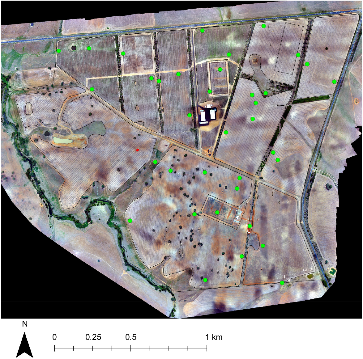
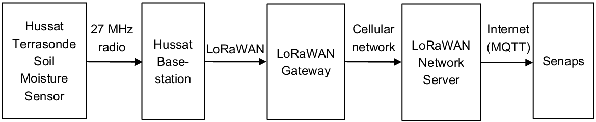
A total of 36 Terrasonde soil moisture probes (Hussat, Hanwood, NSW, Australia; https://hussat.com.au/) were installed at various selected locations across BARS in September 2019 (Fig. 1). These probes have built-in long life internal batteries and short-range underground to surface telemetry. Each probe communicates over a 27-MHz simplex radio link, with a nearby base-station positioned up to 50 m away from the probe, which is solar and battery powered. The relatively low frequency radio signals can penetrate the soil that the probe is buried in. The Hussat Base Station relays the Terrasonde message via a LoRaWAN network to a custom Senaps data ingestion (Fig. 2). Long Range(LoRa) is a physical, non-cellular, wireless technology designed for long-range wireless communication. LoRaWAN, or LoRaWAN wireless Internet of Things (IoT) wide-area network (WAN) protocols, referred to the open, cloud-based protocol and system architecture for IoT networks, which make it possible for LoRa devices to communicate with each other via networks, platforms, and technologies across the Internet.
CSIRO Boorowa Agricultural Research Station (328 km south-west of Sydney, New South Wales in south-eastern, Australia. Green dots, locations of installed soil moisture probes; red square, location of weather station.
Soil moisture sensor data collection, distribution and access pathway for the soil moisture probes located at Boorowa Agricultural Research Station.
Senaps is a cloud-based software platform that provides digital infrastructure for spatio-temporal data and analysis. The platform supports executing user defined analysis models on sensor datasets and allows the data products to be accessible via an Application Programming Interface (API). Flexible permission settings ensure the data is only visible/editable by authorised users. Once data is in the Senaps database, it can be easily value added with the user models. Data consumers can view the value-added data through custom software applications via the API or by using the web interface (https://products.csiro.au/senaps/about/). Senaps is a domain agnostic platform that also facilitates the integration of soil moisture data with other data sources and operational analysis such as crop production simulations and weather observations and forecasting.
The LoRaWAN link has some benefits for transmitting from the Hussat Base Station versus the cellular network in situations where the Hussat Base Station needs to be located outside the range of a cellular network. At BARS, the LoRaWAN Gateway is located at a high point with a high gain antenna and only requires a single SIM card versus needing one for each Hussat Base Station. The LoRaWAN Gateway forwards the sensor messages over the internet to the LoRaWAN Network server. Senaps subscribes to the MQTT (MQ Telemetry, the most commonly used messaging protocol for the IoT) messages from the configured LoRaWAN application and parses the data for storage in its database. LoRaWAN also has benefits over the cellular network in this application as it is more suited to low power, low bandwidth IoT applications without sacrificing transmission distance or security.
The Terrasonde soil moisture probes (Hussat) installed at BARS are 160 cm long and are buried vertically with the top at a depth of 20 cm underground. Each probe has eight sensors measuring soil moisture at 30, 50, 70, 90, 110, 130, 150 and 170 cm. A data reading (soil moisture and temperature) is made from each sensor once every 24 h. The sub-surface position of the top of the sensor ensures on-farm management operations, like planting or cultivation, are not hindered significantly. However, this has obvious implications for measurement and modelling of topsoil (0–20 cm) soil moisture, which is discussed further on.
The location of each probe placement was determined by balancing coverage of environmental variation with needs to minimise disturbances to normal farm operations. For capturing spatial variability, probe installation was determined through kth-order random toposequences (Odgers et al. 2008). Toposequences are generated by taking a random path uphill to the top of a hill and downhill to a stream or valley bottom from a randomly selected seed point. Rather than selecting points along toposequences in some deterministic way, site locations were selected by examining a collection of different pathways and then considering the impact of whether proposed installation would impede normal farm operations. A key factor of consideration was the placement of probe base stations that could be installed up to 50 m from a buried probe. Where regular cropping is practiced on the farm, it was decided that base stations, given their size, be installed to the edge of the cropping fields and consequently, this constrained where several of the probes were installed.
Calibration of the soil moisture sensors
The Terrasonde soil moisture sensors (Hussat) are a capacitance type and measure the relative permittivity (dielectric constant) of the bulk soil surrounding the sensor. It has been shown experimentally that the relative permittivity of soil is highly sensitive to volumetric soil water content (Bogena et al. 2007; Robinson et al. 2008). Permittivity is a physical quantity that describes how an electric field affects and is affected by a dielectric medium (in our case, soil), and is determined by the ability of a material to polarise in response to the field, and thereby reduce the total electric field inside the material.
In general, the relative permittivity is converted to a volumetric water content with a ‘calibration’ equation. The manufacturer of the probes (Hussat) confirmed that the Terrasonde probes operate at 50 MHz. This frequency renders many common calibration equations such as the Topp quadratic function (Topp et al. 1980) and other common equations, such as those described in Gasch et al. (2017) as invalid. Consequently, it is suggested to use a custom calibration that has been developed specifically for the Terrasonde sensors that dually corrects for soil temperature effects on measured soil permittivity readings and provides a measure of volumetric soil water (θ). The set of equations to convert from permittivity (Er) to θ is first to correct for soil temperature effects, followed by parsing this quantity through a defined arithmetic equation with fixed coefficients:
θ is then estimated as:
where ErT and ST are the temperature corrected permittivity and soil temperature respectively. Equation coefficients CF1, CF2, CF3, CF4, CF5 are numerical quantities derived through extensive empirical calibration performed by the manufacturer Hussat and cannot be shared for commercial-in-confidence reasons. Anecdotally the above equations have been successfully applied to similar soil types as found at BARS (Hussat).
Thus, the soil moisture sensors are ‘factory’ calibrated to generate θ values and many users of the sensors are satisfied with the information, knowing values may not reflect actual soil moisture levels, but still demonstrate relative changes in the state of soil moisture. As such, users may apply their own heuristics such as mental models or simple bias corrections to make allowances for these systematic differences irrespective or how large or small they may be. This is often the case for commercially supplied probes. This approach would be considered an ad hoc approach to sensor re-calibration.
Using soil information gathered or modelled at the sites of sensor deployment, Gasch et al. (2017) were able to demonstrate an objective and automated approach to re-calibrate soil moisture sensors to suit them better to the soil conditions in which they are deployed. The Gasch et al. (2017) approach is to match known reference points of the soil moisture characteristic to corresponding points captured along a time series of factory calibrated θ data. A key requirement for this approach is to have a long enough time series to capture events where the sensor experiences both the wet and dry ends of the soil moisture spectrum. The key reference points in relation to the soil moisture characteristic are saturation point, field capacity, and wilting point. Field capacity is a term used interchangeably with drained upper limit, where both are generally identified as the volumetric moisture of a soil at a potential of −1.0 m (McKenzie et al. 2002), or in other words, the maximum amount of water a soil can hold against gravity. Conversely, wilting point corresponds to a soil water content at a potential of −150 m. Crop lower limit is a term often used interchangeably with wilting point, which can often be a source of uncertainty as the ability of different plants to extract water from soils can vary substantially due to physiological differences together with a co-dependence on the soil itself (soil texture, compaction, stratification, crop specific subsoil chemical constraints); the amounts of water in the soil at different depths, which affect root distribution, the transpiration rate of a plant, and the ambient temperature. Thus, the lower limit of a soil is often dependent on the plant type.
In this study, DUL refers to water potentials of −1.0 m (notional field capacity), LL refers to −150 m (notional wilting point), and SAT refers to saturated soil. In addition to having a sufficient time series, an underlying assumption of the Gasch et al. (2017) approach is that the reference points (SAT, DUL or LL) can be easily identified from the time series of sensed soil moisture. In practice, these reference points can be identified along a time series trace by observing the behaviour over time. For example Gasch et al. (2017) scripted an algorithm for identifying DUL by looking for a sharp increase in soil moisture followed by a sharp inflection and then a decrease that stabilised 3–10 days following the inflection point. Similarly, SAT and LL can simply be defined from the maximum and minimum values of the sensor data trace.
After testing, we used a 2-point scaling to re-calibrate the sensor data and established the DUL and LL reference points as the 95th and 5th percentiles of the traces for each sensor after removal of outliers:
where θ* is the re-calibrated θ, DUL are the measured reference points, LL are the modelled reference points, and Upperobs and Lowerobs are the sensor reference points to correspond to DUL and LL, respectively.
Various laboratory and field approaches are established for the measurement of DUL and LL (McKenzie et al. 2002). These all require substantial time, specialised equipment, and expertise to perform. Pedotransfer functions, which use mathematical functions to relate these parameters with more easily acquired soil data are often used in the absence of measurements (Pachepsky et al. 2006). Their application comes with a greater amount of uncertainty, but with appropriate modelling and extension of these models, such pedotransfer functions can significantly reduce time and effort and enhance the amount of data to be made available for a given analysis.
There are several potential pedotransfer function candidates to consider, but the ones we selected in this study were those from Padarian (2014) that were calibrated via genetic algorithms using CSIRO Ecosystem Sciences (APSRU); Agricultural Production Systems Research Unit compilation of 806 soil profiles that includes field measurements of DUL and crop LL for the most commonly grown crops of Australia (Dalgliesh et al. 2012). This is because these pedotransfer functions would be suitable for application on BARS as the calibration represents Australian agricultural soils. For implementation, we have made a general assumption that the measures of crop LL from Dalgliesh et al. (2012) equate to the previously defined concept of LL that is used in this study.
From Padarian (2014), the equation for DUL is:
LL is then estimated as:
where CLAY and SAND are the soil texture fractions for clay (% particles <0.002 mm in diameter) and sand (% particles 0.02–2 mm in diameter), respectively; CEC is cation exchange capacity (meq 100 g−1); and BD is bulk density (g cm−3). Clay, sand, CEC, and bulk density were acquired for each soil moisture probe and sensor using the digital soil data infrastructure from Malone et al. (2022). This entailed intersecting the modelled predictions of the attributes with the point locations of the probes, extraction of the data, then fitting a mass preserving spline soil depth function (Bishop et al. 1999) to the extracted data, to output it such that the sensor locations on the probes were the mid-points of depth intervals down the soil profile. For example, given the above-described positions of the sensors on each probe, soil data were output for the following depth intervals: 0–40 cm, 40–60 cm, 60–80 cm, 80–100 cm, 100–120 cm, 120–140 cm, 140–160 cm, and 160–180 cm. For the first depth at 0–40 cm, it is noted that the top sensor on the probe is 30 cm below the soil surface and does not represent the internal midpoint. This was required due to the absence of a surface soil moisture sensing capability for the present work, and therefore for the top sensor of each probe, we make assumptions that it is measuring the volume of soil in the top 40 cm. It is acknowledged this is an additional source uncertainty to the work described in this research.
With the soil data prepared for each sensor on each probe, Eqns 4 and 5 were applied for estimate DUL and LL, respectively. Eqn 2 could then be applied to re-calibrate the sensor data to adjust θ readings to θ*. The work of identifying the sensor upper and lower limits considered the time series from October 2019 (1 month after sensor installation) to August 2022. For analysis purposes, this time range has been ideal as the soils have experienced severe drought (from end of 2019 to early 2020), and prolonged periods of higher-than-average rainfall (from 2020 to 2022).
Spatio-temporal modelling of soil moisture
The scope of the spatio-temporal modelling for this research was to generate daily soil moisture maps for 1058 days (from October 2019 to August 2022), corresponding to the described depth intervals to 180 cm across BARS at a 5-m grid cell resolution. Volumetric soil moisture is expressed in both cm−3 cm−3 and mm units. Cumulative totals are also generated over each of the intervals. Although not included in this study, cumulative totals can be used at defined depth intervals.
The modelling target variable data for each day are the re-calibrated soil moisture data for each of the eight sensors of the 36 probes. Some processing of these data was performed to identify large data gaps in the temporal record of each sensor. In general, the consistency of the sensor readings was high, but we set a threshold whereby if there were less than 80% of days without a reading, the sensor data stream was removed for all subsequent analysis. Of the 288 candidate data cases, 53 sensor data streams were removed. For the remaining sensor data streams, any missing data were filled in using a cubic smoothing spline before performing a smooth filtering using the Savitsky–Golay smoothing filter (second order polynomial with a window size of 7 days).
Predictive covariates were sourced from the work of Malone et al. (2022) and included those from on-the-go proximal soil survey, which were gamma radiometric data, electromagnetic induction data, and elevation and associated derivatives. To reduce the data layer dimension of these data, principal component analysis was performed, which reduced 14 data layer dimensions to nine while preserving 97.5% of the combined data variation. We also included soil data, specifically estimates of clay content, bulk density, and soil organic carbon. The soil data were harmonised to the depth intervals of the sensor data using the mass-preserving spline depth function from Bishop et al. (1999). Finally, an index value of each depth interval was also included into the predictive covariate suite.
Generalised Additive Models (GAMs; Hastie and Tibshirani 1990) were used to fit daily parameters that related re-calibrated soil moisture data (θ*) with the associated environmental covariate data. To better leverage the temporal dynamics of soil moisture as captured through daily sensor data, the models contained both environmental covariates plus prior model estimates of θ*. Day 1 model covariates included only environmental covariates as those previously mentioned. However, Days 2–7 models contained the same covariates, plus the preceding days model estimates of θ*. For example, the Day 2 model contained environmental covariates plus Day 1 predicted θ*. While Day 7 modelling contained environmental covariates plus θ* prediction for Days 1–6. From Day 8 onwards, the models contained the environment covariates plus the preceding 7 days predicted θ* in a rolling fashion until the end of the modelling period (1058 days).
The somewhat automated approach of the modelling (GAM fitting for each day) called for a side investigation to determine the treatment of predictor variables to use. For GAMs, this entails whether to treat variables as linear predictors or in the case of this study as smoothing spline functions. To do this, manual daily model fitting investigations were done over several consecutive day periods and over different periods across the 1058 days. For each day, a GAM model was constructed in a stepwise fashion, starting by treating each covariate as a linear predictor of the target variable θ*. A scope of model parameter alternatives was then explored via iteration. The model parameter alternatives were smoothing spline functions from one up to five basis dimensions for each covariate. The GAM parameter modelling was set to operate by trying all combinations of the full suite of covariates and their linear and smoothing parametrisations until the whole modelling scope was explored. We note that each covariate was introduced once to a model, either as a linear or smoothing spline variable, never combinations of both. The parameter set that returned the smallest Akaike Information Criterion (AIC) value was selected as the ‘final’ model. From this analysis, for the daily model fitting automation process, five of the nine environmental covariates were to be treated as linear predictor variables. The other four were to be treated as smoothing spline functions with either four or five basis dimensions. The soil variables were to be treated as linear predictors, and prior soil moisture data were to be treated as smoothing spline functions with three basis dimensions for each day.
Due to the relatively small number of cases (233), 90% were used for model calibration for each day of modelling. The remaining 10% of data were used to evaluate the goodness of model fit. Lin’s Concordance correlation (CCC) and the root mean square error of prediction (RMSE) were the selected metrics used for model evaluation. The fitted model was then put into prediction mode and used for extension to grid predictor variables and create digital maps of soil moisture for each of the defined soil depth interval layers.
Implementation of methods
All data analysis was performed using R (R Core Team 2022). For all spatial and GIS operations, sp (Pebesma and Bivand 2005), rgdal (Bivand et al. 2022), and raster (Hijmans 2022) were used. GAM modelling used a combination of the gam (Hastie 2023) and mgcv (Wood 2004) packages. The stepwise GAM procedure was performed using the gam package using the step.Gam function.
Results
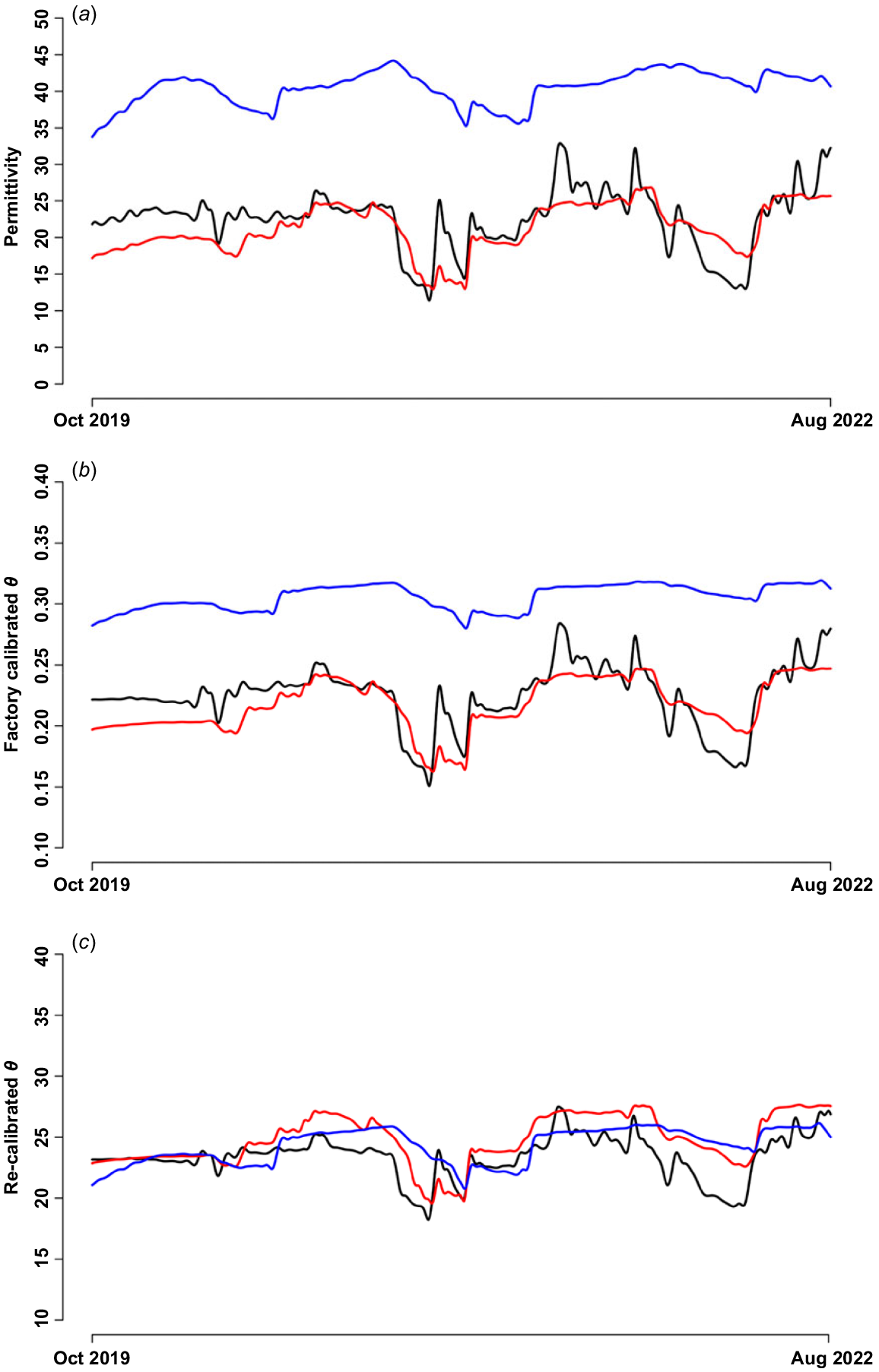
Each of the soil moisture probes and their sensors across the whole SMSN output daily permittivity readings. Our workflow then processes these readings in combination with associated soil temperature readings, then applies an initial factory calibration equation to derive θ estimates. This is followed by re-calibrating those estimates via a 2-point scaling by matching given sensor readings with associated site characterised soil information related to the hydraulic properties (DUL and LL). Both DUL and LL were estimated by pedotransfer function, and we selected near maxima and minima of the sensor estimates of θ to these soil hydraulic variables respectively. Fig. 3a shows the permittivity reading from three sensors (30 cm, 90 cm, 150 cm) of a single probe over the course of the 1058-day study period. Compared with Fig. 3b that shows the soil moisture data in θ units, the permittivity data is less smooth, which is due to the diurnal changes in the readings due to soil temperature variations. The factory calibration effectively smoothed these out, while also performing a systematic adjustment. As expected, the 30-cm data are temporally more variable than the 90-cm data, which again is also more variable than the 150-cm data due to differences in the dynamics of plant–soil water interaction down a soil profile. To provide some local context, the soils across the farm are predominantly lighter topsoils (clay loams), about 25 cm thickness above light to medium clay soils with measurable amounts of gravel. The soil moisture sensing is mainly measuring the clayey component of the soil, beneath the sandier upper horizons, which means that we expect similar values of DUL and LL at deeper sensor depths. In the sensor re-calibration, particularly for the 150-cm sensor, the re-scaling brings the soil moisture trace into the similar upper and lower range as for the other sensors. The re-calibration does not affect the pattern of the data, and Fig. 3c shows the delayed wetting and drying at lower depths in the soil profile is in response to inputs from rain and crop water usage over time.
Soil moisture traces from sensors located at 30 cm (black line), 90 cm (red line), and 150 cm (blue line) for a selected soil probe (#142). (a) Raw sensor permittivity readings for (b) factory calibrated soil moisture and (c) re-calibrated soil moisture.
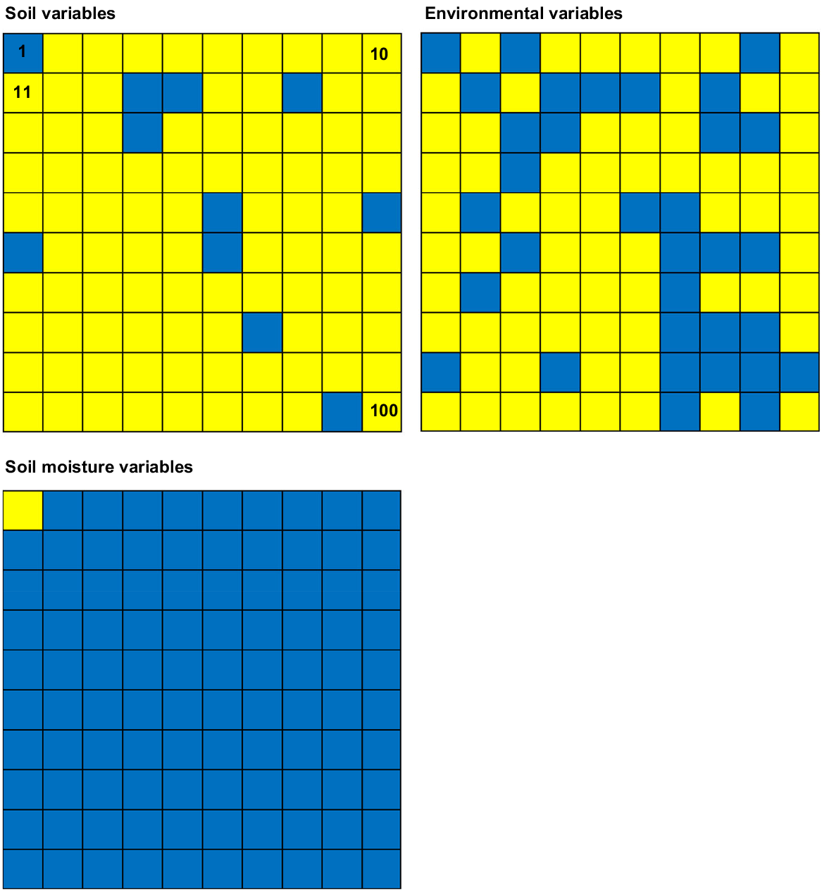
Spatial modelling used daily fitted GAMs to model soil moisture at specified depth intervals down to 180 cm. The predictor variables included covariates derived from proximal soil sensing (environmental variables), digital soil mapping (soil variables) and time lagged (up to 7-day history) prior soil moisture estimates. As a simple sensitivity analysis to get a sense of which predictors have a relatively strong association with real time soil moisture. To determine significant differences, we assessed the P-values for each fitted model parameters. Using a 0.05 threshold across each day, we summarised which variables (soil, environmental, and prior soil moisture) were identified as being significant. Fig. 4 shows for the first 100 days those variables that were model significant (blue squares). Soil variables (clay, soil carbon, bulk density and depth interval) were used infrequently. On the first day of the analysis, we expected an association. However, the environmental variables were used more frequently, but the pattern is difficult to interpret and does not relate to other factors such as rainfall. The use of prior soil moisture is significant in each of the models, except the first day when it was not included in model. This general pattern is consistent across the 1058 days of the study. As the modelling after Day 1 contains prior estimates of soil moisture, those estimates also capture the initial associations between observed soil moisture and the soil and environmental covariates from Day 1 and continue for 1058 days. Hence, specific parameter significance for the soil and environmental variables is only sporadic, but nevertheless provide and important inclusion over the course of the model runs.
Model predictor variable themes (soil, environmental, and prior soil moisture), which were identified as being significant (blue squares) over the first 100 days of the GAM modelling system. Blocks are to be read from the top left corner (Day 1), then row wise down to the bottom right corner (Day 100).
Regarding the soil moisture covariates, the frequency of their significant association was different depending on the length of the time lag. The 7-day historical soil moisture prediction was included in 100% of models after 8 days of running the automated modelling. A total of 61% of days included historical soil moisture predictions from Day 6. For Days 1, 2, 3, 4, and 5, the historical soil moisture covariates were significantly associated at 23%, 20%, 20%, 21%, and 25% of the time, respectively. The more significant associations with soil moisture covariates with 6-day and 7-day lags might indicate that genuine patterns of temporal variation of soil moisture are not revealed till a certain quantum of days has passed between measurements. On a day-to-day scale, changes in soil moisture are small relative to changes over a week.
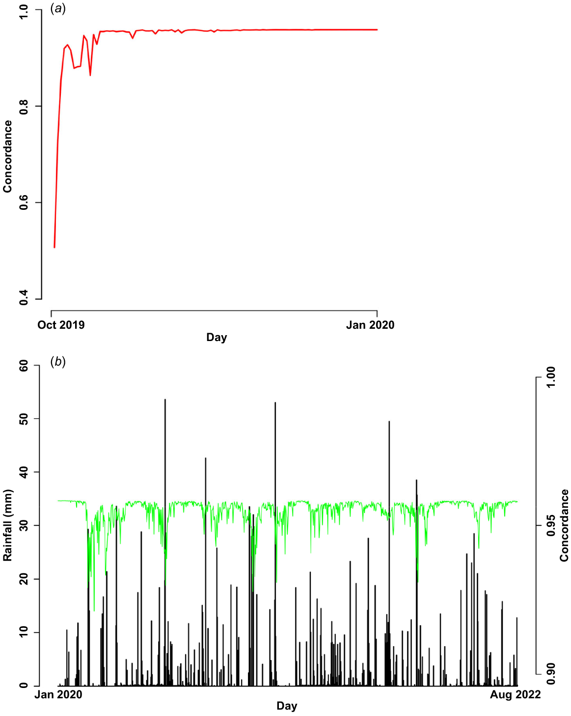
Fitted models were evaluated each day using an out-of-bag dataset, 10% of the available data cases. This out-of-bag dataset was selected at random each day of the modelling. Fig. 5a shows the change in concordance estimates between measured and estimated soil moisture based of the out-of-bag data for the first 100 days. After the first day where a concordance of about 0.5 was found, it increased substantially, then fluctuated somewhat for 2–3 weeks before stabilising to about 0.96. RMSE also stabilised around to 0.002 cm−3 cm−3. During this time, rainfall was not being recorded at the farm. From January 2020 to August 2022, a plot of the relationship between rainfall (measured at a single monitoring station on the farm; Fig. 1), and model concordance was investigated. While one might expect rainfall patterns experienced at each soil moisture probe location to be different than at the site of the weather monitoring station, the visual patterns observed between rainfall and model concordance exhibit an interesting but not overly strong relationship (Fig. 5b). While model concordance does not fall below 0.9, where it does fall, there is a general correspondence during periods of higher rainfall. There would be expected a variable pattern of rainfall to be experienced across the farm, and therefore not all sensors would be reading uniform amounts of water entering the soil. While the models eventually stabilise, the incidence of rainfall inputs to the soil temporarily confuse the modelling, as there is no variable or covariate in the model that is directly accounting for the variation attributed to rainfall, excepting of the historical soil moisture predictions, but this relationship would be irregular given time lags for moisture to be entering and moving down into the soil and effects due to evapotranspiration (Jensen and Pedersen 2005).
(a) GAM model evaluation concordance for the first 100 days (October 2013–January 2020). (b) GAM model evaluation concordance together with observed rainfall measured at weather station (January 2020– August 2022).
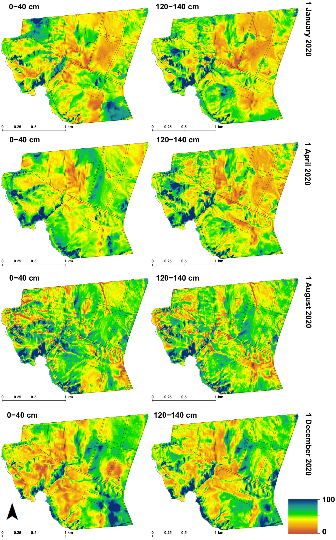
To visualise the temporal nature of the digital soil mapping products, we show selected time snapshots during the 2020 calendar year for the 0–40 cm and 120–140 cm depth intervals (Fig. 6). The start of 2020 was particularly dry with widespread areas of the farm being less than 25% full relative to available water capacity, though much spatial variation exists due to differences in terrain and soil properties. Nevertheless, both upper and lower depth intervals are similar in terms of soil moisture content. Rainfall in March 2020 led to widespread increases in soil moisture, but mainly observed nearer to the soil surface as seen in maps of April 2020. It was not until August 2020 that widespread soil moisture in both upper and lower depths was observed. Soil drying down is observed for the upper depth interval in December 2020, and less so for the lower depth interval. While these observations can be made for the give four time points only in Fig. 6, we developed a shiny application (https://shiny.esoil.io/Apps/BARS_SM/) that displays daily mapping for each depth interval as well as cumulatively in both cm−3 cm−3 and mm soil moisture units. These maps provide an indication of the soil moisture spatio-temporal variability across the farm, and highlights the differences in soil attributes and landscape features to show that the pattern of soil moisture is not uniform through time.
Mapped estimates of soil moisture relative to available water capacity, expressed as a percentage for 0–40 cm and 120–140 cm depth intervals. These maps are shown for the specific time points of 1 January 2020, 1 April 2020, 1 August 2020, and 1 December 2020.
To provide an operational soil moisture mapping data service for BARS, a version of the above described spatio-temporal modelling software and data are hosted within the Senaps platform. Senaps provides a scientific workflow hosting capability to operationalise sensor data analysis. The Senaps workflow system allows the combination of heterogeneous computational operators into complex workflows. Users of the platform can upload their analysis code without the intervention of platform administrators or developers. The soil moisture modelling analysis described above and implemented in R code was uploaded to the platform and is then available to authorised users as an operator that can be instantiated in a data Workflow in Senaps. The operator software package provides meta-data to the software platform to describe the base software image, software library dependencies (include R packages and system libraries) and the inputs and outputs of the operator. The operator package also includes static datasets utilised in the analysis but not dynamically updated. The operator is instantiated as a workflow using a graph describing the input and output data locations within the platform. Each time the workflow execution is required the Senaps platform will retrieve the code and deploy the required computational infrastructure.
To operate effectively, additional functionality is added to support operating in a near real time context. These functions allow the analysis software to determine the availability of new input data and incrementally generate new daily outputs as required. In addition, the underground and low power design of the soil moisture sensors mean that samples can be delayed by transient communication outages. The data availability thresholds described above are also applied in the operation workflow; however, on a sliding temporal window defined by the schedule. The workflow is deployed on two schedules: (1) one that is scheduled every second day to ensure the output soil moisture maps are available with low latency for operational use; and (2) one that is scheduled each month where the past 30 days is reprocessed to ensure the final time series is derived from all possible sensor samples. Since GAM modelling used in this analysis requires the preceding 7 days of model estimates of θ* and the Senaps platform deploys compute infrastructure on demand. At each scheduled execution, the operator code can first retrieve the preceding 7 days of output data before calculating the newly added days of output estimates for θ*.
The operational soil moisture workflow generates output data in multiple formats including a time series of numerical GeoTIFF files and RGB GeoTIFF files for visualisation purposes and a multi-dimensional NetCDF to allow efficient timeseries extraction. The output files are made available for access by researchers and external software tools such as GIS software using APIs provided by the THREDDS software included within the Senaps platform.
Discussion
Deriving value from SMSNs is an actively growing area of work and research, given the impact of available soil moisture for productive agriculture. Various tools and platforms are available in the marketplace and being developed in research (Gallacher et al. 2023) to proffer insights that will aid in on-farm decision making. In this research, additional value is added to a SMSN through spatio-temporal modelling that generates daily soil moisture maps. The mapping provides the visual tool that evaluate differences between sensors due to changes in soil attributes and non-uniformity of inputs such as via rainfall or irrigation. The sorts of inferences that may be derived from single probe analysis tools could easily be incorporated into a mapping system, enriching the suite of insights that can be derived due to the spatial nature of the data.
The primary goal of this work was to describe the processes needed from establishing a soil SMSN, collecting and processing the raw sensor data, and spatio-temporal modelling of the processed data. What was described is not the only way of generating daily soil moisture mapping, but provides some cues for others with similar networks to derive additional value from them. The intention was to build a system that would be considered operational, such that insights can be immediately delivered. From this, further innovation via improvements to execution of key steps can be easily incorporated later. The following discussion provides some justification for choices made in developing the operational system and then points out several tasks, or alternative procedures whereby improvements in mapping precision are to be expected or might be achieved or not.
Re-calibration of soil moisture probes
For mapping of soil moisture, the importance of site-specific calibration of each probe and sensor across the SMSN cannot be understated. Sensor re-calibration takes into consideration the collective expression of soil attributes at the site of the probe installation. From a mapping perspective, this enables one to exploit correlative relationships between sensors (autocorrelation) and with other soil and landscape features. Even with rudimentary soil and landscape information to drive the spatio-temporal modelling workflow, one can expect the expression of soil moisture variations to be driven by known soil and landscape processes. When there is highly granular soils information as used in this work, the expression of soil moisture and soil–landscape relationships becomes more enhanced.
Yet, there is considerable uncertainty in the way sensor re-calibration is done. This is because there is the implied assumption about the relationship between near upper and lower sensor readings corresponding to DUL and LL. Naturally, this is a convenient concept. Based on sensor experiences from both extremes of the soil moisture characteristic, and from an operational perspective, the established sensor upper and lower reading (e.g. Gasch et al. 2017) are likely to be close enough to DUL and LL, respectively. More pertinent is the issue with the measurement or estimation of DUL and LL. To avoid characterisation of DUL and LL, sensor re-calibration may entail the taking of soil moisture measurements either in the laboratory or field and corresponding these with the sensor readings taken at the same time as measurement. This is a very large and complex undertaking, and the effort multiplies as probe and sensor number increases. The degree of difficulty also increases especially in the field, and more so when investigations are done at increasing depth below the soil surface. Performing the same work in the laboratory removes the difficulties encountered in the field. However, new problems are introduced, such as the wetting up and drying down of soil needs to be done in a controlled environment, which requires specialised equipment. There are also issues if analysis is performed using re-packed soils rather than in situ soil material (Sakaki and Smits 2015). Furthermore, there is the need to have soil moisture sensors integrated into the laboratory process. Therefore, establishing a measurement (better) or prediction (less better) of DUL and LL is a more practicable route to follow.
Measuring or predicting DUL and LL
Measurement of DUL and LL is not without difficulty. In the field, this may entail the opportunistic approach, especially in years where there is good early-season and within-season rainfall. Ensuring a soil profile is at DUL is relatively easier to manage in uniform heavier textured soils, but uncertainty increases for lighter textured soil (as the window of opportunity narrows), or soils that express a soil texture contrast. Integration with watering and neutron probe observations (assuming it is correctly calibrated) is one way to circumvent this issue (Burk and Dalgliesh 2013). For LL (or CLL in this case), even with rain-out shelters installed at anthesis, one can only confidently characterise a whole soil profile in a particularly dry year in texture contrast soils. Collectively, the implication is that it may take more than 1 year for each probe to acquire confident measures of DUL and LL via the opportunistic approach. Ongoing efforts at BARS are seeking to establish these data in any case. Alternatively, or perhaps in conjunction with opportunistic approach, is via laboratory work using suction tables and pressure plates to measure either the full soil moisture characteristic or just for the desired pressure potentials that DUL and LL are commonly attributed. Where soil cores are re-packed instead of in-field condition, the efficacy of such methods also needs to be considered.
Clearly, even the measurement of soil moisture and DUL and LL are potentially fraught with uncertainties, and not even through measurement alone, but other factors such as whether done in field or laboratory. However, measurement is more ideal than prediction, whereby the meaning of prediction is via pedotransfer functions that establish relationships between relatively easier to characterise soil attributes and the target variables of interest (DUL and LL that a comparatively much more difficult to characterise). In this study, we adopted equations from Padarian (2014) on the basis they were derived from predominately agricultural soils from around Australia. Like earlier discussions about the needed for re-calibration of soil moisture sensors to better match with in situ conditions, pedotransfer functions are equally limited in terms of their extensibility outside the range of data they were fitted with. Here, the issue is not likely the geographic and edaphic range of the pedotransfer functions; rather, it is their sensitivity to changes in soil attributes at a local or farm scale. Anecdotally from some measurements we have acquired from BARS, the pedotransfer functions used in this study correspond quite well with DUL but underpredict LL and are not very sensitive to changes in soil texture spatially and laterally, which equate the smoother than expected maps of DUL and LL.
However, the convenience of adopting a pre-existing pedotransfer function and integrating into the modelling system is not to be overlooked as it enabled its efficient creation. This is one part of the whole modelling system that can be easily improved in future updates where in the first instance, efforts be directed toward developing farm specific pedotransfer functions that in themselves can grow more precise as new measurement data is continually added to them. Taken together with routine visitation of the sensor upper and lower reading limits, we see a continual revisit and feedback approach to ongoing updates to improve DUL and LL characterisation, and ultimately, greater precision of soil moisture monitoring at each probe location.
Spatio-temporal modelling
Once soil probes have been re-calibrated, the daily recording of these data are brought into a spatio-temporal modelling system. We previously highlighted the various sources of uncertainty that is attributed to these data, yet in this work, there is no attributable uncertainty incorporated into the spatio-temporal modelling. The assumption is that the data is free from error. Future iterations of the modelling systems will obviously attempt to address this wrong assumption. Another of the big assumptions is the absence of soil moisture measurement at the soil surface, and the solution to account for this by attributing the measurements from the top sensor of each probe (positioned 30 cm below soil surface) to be representative of the top 40 cm. In general, we have established that the sensor position is located at the midpoint of a depth interval. For convenience, this is helpful to do as it enables estimation of soil available water in mm units and allows the calculation of integrals across any depth intervals and ranges. However, the issue of surface soil moisture is not rectified, given the greatest fluxes are observed at the surface. Operationally, this is actively being addressed by the installation of co-located surface probes that can be easily removed during field activities such as seeding, fertiliser application and harvesting. The work of re-calibration we have previously described need to be performed before these additional probes are integrated into the system. A point of exploration is the integration with remote and proximal sensing platforms that actively measure soil moisture and is part of future research efforts to fuse both data source types.
The decisions for selection of spatio-temporal modelling structure were considered in terms of whether the modelling process could be automated and performed relatively efficiently. The appropriateness of selected model for the quantity of data available was also considered, which entailed decisions around selection of model type and suitability to use for temporal modelling. Another factor was a preference to use modelling workflows commonly performed for digital soil mapping that potentially includes several predictive covariates. Machine learning was considered but was eliminated together with other approaches such as formal linear and non-linear spatio-temporal modelling frameworks because of suitability to uses with the available size of data, the difficulty to automate in a daily time step fashion, model complexity and interpretability. The practical solution therefore was to adopt the use of GAMs as they facilitate investigation of non-linear association between covariates and target variable and fitted adequately to the other criteria that was required.
The inclusion of rolling 7-days prior soil moisture estimates into modelling facilitated the capture of temporal variation in soil moisture and the interaction between soil moisture and soil and landscape features. While it was an ad hoc decision to select a rolling 7-day historical period, rather than 2, 3, 14 or even 21 days, the created modelling system can be adapted and optimised in future iterations, which may sensitivity test this feature. Alternatively, it might be possible to adopt another approach such as temporal weighting that gives near real time dynamic covariates (soil moisture predictions, in the case of this study) higher weighting than more historical dynamic covariates (Heuvelink et al. 2021). Given that our own analysis revealed relatively stronger predictive power of soil moisture covariates to those 6 or 7 days prior rather than to Day 1 or 2 prior, due consideration of this approach would need to be considered.
Considerations for establishing and maintaining an on-farm soil moisture sensor network
Technical improvements to the created soil water monitoring system were described above. The following general discussion considers aspects of an on-farm SMSN related to establishment and its ongoing maintenance.
In the establishment of the SMSN with 36 probes distributed across BARS, considerations were made about their placement with the intention of capturing the expressed soil and environmental variability to ensure the best possible spatio-temporal model extension. The determination of installing 36 probes was not guided by any statistical inference or optimisation but like in most other contexts, was defined by other measures such as costs, project time constraints, and manufacturer considerations. Having 36 probes installed across a 290-ha farm would be considered on the upper end of soil moisture sensing capability. From a purely modelling perspective where more data is better, there is an inclination to try to increase the density. There are statistical approaches readily available to explore what an optimal number might be. However, most operators or land managers thinking of establishing a SMSN perhaps would not consider having a density of one probe every 6 ha, as at BARS. Having only one or two sensors across a farm will not enable the spatio-temporal modelling described in this work, though some general recommendations can be made if the intention is to produce mapping. The actual number is probably less important than the actual placement. Of great importance is an understanding of whether acquired knowledge or detailed mapping of the soil and landscape that the farm is situated on. Delineating zones of common soils can then be performed, which allow sensor/s to be installed in each of them. Even installing a single sensor in each zone will provide some spatio-temporal insight in soil moisture fluxes. With greater numbers of sensors installed, there is increased ability to exploit modelling capabilities, as well as more granular information about the soil and landscape.
Due to the the tendency to set-and-forget, the ongoing maintenance of a SMSN is often overlooked. This is problematic as the ongoing physical maintenance needed to keep the probes operational, and the ongoing supporting data infrastructure system also needs to be carefully planned. This includes alert and integrity checking systems to inform operators of malfunctioning equipment or data streams, and scheduling tools to record, monitor and update their ongoing maintenance. Soil moisture probes also have an end-of-life due to battery constraints or just through long-term operational use in difficult environments. Decisions are needed to either replace a probe or install a new one at the same location; or perhaps install a new probe in an entirely new location. An argument for the latter option is that over the life of an installation, a thorough understanding of the behaviour of soil and soil moisture fluxes will have been well established and predictable. For example, sufficient information may indicate that monitoring is no longer needed at a particular site, and there is more need to relocate it elsewhere. As more and more SMSNs become established, these questions and considerations will eventuate more often, and to ensure the most benefit is gained from a large financial investment, set-and-forget strategies are not feasible.
Conclusions
In this study, our intention was to step through the processes needed to enrich insights that might be gained by having an on-farm soil moisture sensing network. The benefits of real time tracking of soil moisture are obvious for several land management contexts. The spatio-temporal mapping of soil moisture combines what is observed from a network of points with granular insights of soil and landscape process and attributes to give clear and visual understanding of soil moisture fluxes across a farm. By the process of building an operational on-farm soil moisture monitoring system, the core processes needed can be established. We discussed the processes of sensor installation, underpinning data collection infrastructure, the necessary data analytics involving sensor calibration and re-calibration, and spatio-temporal modelling and mapping. What was created is not a final product, but the first of an iterative system whereby the efforts of the data analytics pipeline involving sensor calibration and modelling be revisited and improved. A range of options for sensor re-calibration revolves around better characterisation of soil DUL and LL ranging from relatively straightforward (improving pedotransfer functions) to more difficult and costly (field and lab measurement). Many options can be entertained for spatio-temporal modelling, but it is important to consider not just the elegance of the modelling but the practicality of the model to be suited for the context, which in our case was daily, granular estimates of soil moisture. Nevertheless, the whole predictive system generated in this study is modular and therefore easier to revisit and improve each component individually when there is a need.
On-farm soil moisture sensing is an ever-increasing practice and is an indication of the broader digitalisation of farming. While the digital farming ecosystem is emerging, the temptation with nearly all components of the digital infrastructure is to set-and-forget. Rather, a longer view and plan is needed for the ongoing maintenance and improvement of such systems so that we can derive full value and insights from them.
CRediT author statement
Brendan Malone B: Conceptualisation, Methodology, Formal Analysis Investigation, Writing – Original Draft, Writing – Review and Editing. David Biggins: Software, Resources, Data Curation, Writing – Review and Editing. Chris Sharman: Software, Resources, Data Curation, Writing – Review and Editing. Ross Searle: Conceptualisation, Methodology, Software, Writing – Review and Editing. Mark Glover: Investigation, Resources, Writing – Review and Editing. Stuart Brown: Investigation, Resources, Writing – Review and Editing.
Data availability
Real time and historical soil moisture data for each of the probes used in this study may be access through the SENAPS platform dashboard (https://senaps.io/dashboard/#/app/stream/all). An account will first need to be established with the SENAPS team (https://products.csiro.au/senaps/about/) to access those data. The digital soil mapping data that support this study will be shared upon reasonable request to the corresponding author.
Acknowledgements
The authors acknowledge the CSIRO Agriculture and Food business unit internal Digital Research Farms strategic investment for the operating and personnel support that made this research possible. We also acknowledge CSIRO colleagues Sebastian Ugbaje and James Moloney for their technical reviews during the drafting of this document.
References
Bishop TFA, McBratney AB, Laslett GM (1999) Modelling soil attribute depth functions with equal-area quadratic smoothing splines. Geoderma 91(1), 27-45.
| Crossref | Google Scholar |
Bivand R, Keitt T, Rowlingson B (2022). rgdal: Bindings for the ‘Geospatial’ Data Abstraction Library. Available at https://CRAN.R-project.org/package=rgdal
Blaschek M, Roudier P, Poggio M, Hedley CB (2019) Prediction of soil available water-holding capacity from visible near-infrared reflectance spectra. Scientific Reports 9, 12833.
| Crossref | Google Scholar |
Bogena HR, Huisman JA, Oberdörster C, Vereecken H (2007) Evaluation of a low-cost soil water content sensor for wireless network applications. Journal of Hydrology 344(1), 32-42.
| Crossref | Google Scholar |
Bogena HR, Weuthen A, Huisman JA (2022) Recent developments in wireless soil moisture sensing to support scientific research and agricultural management. Sensors 22, 9792.
| Crossref | Google Scholar |
Brown WG, Cosh MH, Dong J, Ochsner TE (2023) Upscaling soil moisture from point scale to field scale: toward a general model. Vadose Zone Journal 22(2), e20244.
| Crossref | Google Scholar |
Burk L, Dalgliesh N (2013) Estimating plant available water capacity. GRDC. IBSN 978-1-875477-84-5. Available at https://www.apsim.info/wp-content/uploads/2019/10/GRDC-Plant-Available-Water-Capacity-2013.pdf
Campbell JE (1990) Dielectric properties and influence of conductivity in soils at one to fifty megahertz. Soil Science Society of America Journal 54(2), 332-341.
| Crossref | Google Scholar |
Dalton FN, Van Genuchten MT (1986) The time-domain reflectometry method for measuring soil water content and salinity. Geoderma 38(1), 237-250.
| Crossref | Google Scholar |
Gallacher D, Roth G, McBratney A (2023) Interactive soil moisture interface of multi-depth change over time. Computers and Electronics in Agriculture 204, 107508.
| Crossref | Google Scholar |
Gasch CK, Brown DJ, Brooks ES, Yourek M, Poggio M, Cobos DR, Campbell CS (2017) A pragmatic, automated approach for retroactive calibration of soil moisture sensors using a two-step, soil-specific correction. Computers and Electronics in Agriculture 137, 29-40.
| Crossref | Google Scholar |
Hastie T (2023) gam: Generalized Additive Models. Available at https://CRAN.R-project.org/package=gam
Heuvelink GBM, Angelini ME, Poggio L, Bai Z, Batjes NH, van den Bosch R, Bossio D, Estella S, Lehmann J, Olmedo GF, Sanderman J (2021) Machine learning in space and time for modelling soil organic carbon change. European Journal of Soil Science 72, 1607-1623.
| Crossref | Google Scholar |
Hijmans RJ (2022) raster: Geographic Data Analysis and Modeling. Available at https://CRAN.R-project.org/package=raster
Huth NI, Poulton PL (2007) An electromagnetic induction method for monitoring variation in soil moisture in agroforestry systems. Australian Journal of Soil Research 45, 63-72.
| Crossref | Google Scholar |
Jensen NE, Pedersen L (2005) Spatial variability of rainfall: Variations within a single radar pixel. Atmospheric Research 77(1), 269-277.
| Crossref | Google Scholar |
Jung HC, Kang D-H, Kim E, Getirana A, Yoon Y, Kumar S, Peters-lidard CD, Hwang EH (2020) Towards a soil moisture drought monitoring system for South Korea. Journal of Hydrology 589, 125176.
| Crossref | Google Scholar |
Kean WF, Waller MJ, Layson HR (1987) Monitoring moisture migration in the vadose zone with resistivity. Groundwater 25, 562-571.
| Crossref | Google Scholar |
Malone B, Stockmann U, Glover M, McLachlan G, Engelhardt S, Tuomi S (2022) Digital soil survey and mapping underpinning inherent and dynamic soil attribute condition assessments. Soil Security 6, 100048.
| Crossref | Google Scholar |
McColl KA, Alemohammad SH, Akbar R, Konings AG, Yueh S, Entekhabi D (2017) The global distribution and dynamics of surface soil moisture. Nature Geoscience 10(2), 100-104.
| Crossref | Google Scholar |
Odgers NP, McBratney AB, Minasny B (2008) Generation of kth-order random toposequences. Computers & Geosciences 34(5), 479-490.
| Crossref | Google Scholar |
Pachepsky YA, Rawls WJ, Lin HS (2006) Hydropedology and pedotransfer functions. Geoderma 131(3), 308-316.
| Crossref | Google Scholar |
Pebesma EJ, Bivand RS (2005) Classes and methods for spatial data in R. R News 5(2), 9-13.
| Google Scholar |
Petropoulos GP, Ireland G, Barrett B (2015) Surface soil moisture retrievals from remote sensing: current status, products & future trends. Physics and Chemistry of the Earth, Parts A/B/C 83–84, 36-56.
| Crossref | Google Scholar |
R Core Team (2022) R: A language and environment for statistical computing. R Foundation for Statistical Computing, Vienna, Austria. Available at https://www.R-project.org/
Rhoades JD, Raats PAC, Prather RJ (1976) Effects of liquid-phase electrical conductivity, water content, and surface conductivity on bulk soil electrical conductivity. Soil Science Society of America Journal 40(5), 651-655.
| Crossref | Google Scholar |
Richards LA, Gardner W (1936) Tensiometers for measuring the capillary tension of soil water. Agronomy Journal 28(5), 352-358.
| Crossref | Google Scholar |
Robinson DA, Campbell CS, Hopmans JW, Hornbuckle BK, Jones SB, Knight R, Ogden F, Selker J, Wendroth O (2008) Soil moisture measurement for ecological and hydrological watershed-scale observatories: a review. Vadose Zone Journal 7(1), 358-389.
| Crossref | Google Scholar |
Sakaki T, Smits KM (2015) Water retention characteristics and pore structure of binary mixtures. Vadose Zone Journal 14(2), 1-7.
| Crossref | Google Scholar |
Topp GC, Davis JL, Annan AP (1980) Electromagnetic determination of soil water content: measurements in coaxial transmission lines. Water Resources Research 16(3), 574-582.
| Crossref | Google Scholar |
Visvalingam M, Tandy JD (1972) The neutron method for measuring soil moisture content–A review. Journal of Soil Science 23(4), 499-511.
| Crossref | Google Scholar |
Wadoux AMJC, McBratney AB (2021) Digital soil science and beyond. Soil Science Society of America Journal 85, 1313-1331.
| Crossref | Google Scholar |
Wood SN (2004) Stable and efficient multiple smoothing parameter estimation for generalized additive models. Journal of the American Statistical Association 99(467), 673-686.
| Crossref | Google Scholar |