

Monitoring tropical freshwater fish with underwater videography and deep learning
Andrew Jansen A * , Steve van Bodegraven A , Andrew Esparon A , Varma Gadhiraju B , Samantha Walker A , Constanza Buccella A , Kris Bock B , David Loewensteiner A , Thomas J. Mooney A , Andrew J. Harford A , Renee E. Bartolo A and Chris L. Humphrey A
A
B
Abstract
The application of deep learning to monitor tropical freshwater fish assemblages and detect potential anthropogenic impacts is poorly understood.
This study aimed to compare the results between trained human observers and deep learning, using the fish monitoring program for impact detection at Ranger Uranium Mine as a case study.
Fish abundance (MaxN) was measured by trained observers and deep learning. Microsoft’s Azure Custom Vision was used to annotate, label and train deep learning models with fish imagery. PERMANOVA was used to compare method, year and billabong.
Deep learning model training on 23 fish taxa resulted in mean average precision, precision and recall of 83.6, 81.3 and 89.1%, respectively. PERMANOVA revealed significant differences between the two methods, but no significant interaction was observed in method, billabong and year.
These results suggest that the distribution of fish taxa and their relative abundances determined by deep learning and trained observers reflect similar changes between control and exposed billabongs over a 3-year period.
The implications of these method-related differences should be carefully considered in the context of impact detection, and further research is required to more accurately characterise small-growing schooling fish species, which were found to contribute significantly to the observed differences.
Keywords: artificial intelligence, biodiversity, channel billabong, computer vision, convolutional neural network, Kakadu National Park, object detection, Ramsar wetlands.
Introduction
Environmental monitoring and assessment are critical in informing management actions necessary to maintain ecological, cultural and socioeconomic values as anthropogenic activities place increasing pressures on aquatic ecosystems (Nichols and Williams 2006). Monitoring biological community composition informs the status or ‘health’ of an ecosystem as well as spatial and temporal patterns in biological diversity across a landscape.
Advances in methods used to monitor aquatic systems are transforming our ability to measure ecosystem change with increasing temporal frequency, spatial resolution and spatial scales. Techniques such as species detection using DNA metabarcoding (Hebert et al. 2003; Bush et al. 2019), aquatic vegetation mapping using multi-spectral satellite imagery (Whiteside and Bartolo 2015) and fish surveys using underwater cameras (King et al. 2018; Follana-Berná et al. 2020; Hannweg et al. 2020) have introduced more accurate, efficient or safer ways of collecting, storing, managing, and processing and analysing ecological data.
In Kakadu National Park (KNP) and enclosed mining leases in northern Australia, tropical freshwater fish communities have been monitored since 1988 to ensure they are protected from the potential effects of uranium mining in the region (Bishop et al. 1995; Humphrey et al. 2016). This monitoring record represents one of the longest interannual studies of freshwater fishes in Australia’s wet–dry tropics. Owing to the seasonal variation in hydrology associated with wet–dry tropical ecosystems, fish assemblages are measured annually during receding flows. This wet–dry transition phase is the period that summates potential impacts associated with antecedent wet season mine-water dispersion to ecosystems, the period of maximum biological diversity, first access to sampling sites and high clarity of surface waters for visual observations, and the most stable period in fish community composition, with minimal influences from fish migration in or out of refuge waterbodies that become isolated (Humphrey et al. 1990). Detection of potential impact is made predominately using calculations of paired site Bray–Curtis dissimilarity with a before–after–control–impact (BACI) experimental design, where control and exposed waterbodies are annually compared using multi-factor PERMANOVA with current and previous years (Supervising Scientist Division 2011a, 2011b).
Fish monitoring methods in Kakadu streams have recently transitioned (in 2016) from visual observation to underwater videography, with early developmental results reported in King et al. (2018). Videography was primarily introduced to reduce the risk to boat-based observers from saltwater crocodiles, but the benefits are far-reaching, including a decrease in the number of people and time required for field operations, as well as the creation of a permanent, recorded dataset that can be revisited as new analysis techniques are developed. New metrics to measure community structure have emerged as a result of the adoption of videography to monitor fish, such as MaxN, which is the maximum number of fish in a species population present in one video frame (Cappo et al. 2001; Whitmarsh et al. 2017). Using underwater videography instead of traditional visual observation survey techniques also represents a significant shift in terms of format, and increase in electronic data size and complexity.
Deep learning or deep neural networks are a popular tool for processing and analysing ‘big data’ (Shen 2018). Big data are large or complex datasets and may be difficult to analyse using traditional data analysis methods (Dafforn et al. 2016). Deep neural networks can recognise complex patterns in non-linear data, with high predictive performance (Almeida 2002), and are being used effectively in the field of computer vision to train models for visual recognition tasks (Khan et al. 2018). Implementing deep learning algorithms has been made easier for practitioners without extensive coding experience because of the emergence of software tools that facilitate image preparation and model training using a click-and-deploy graphical user interface (GUI) (Del Sole 2018; Liberty et al. 2020). This frees up time to focus on the critical task of generating training datasets rather than developing custom neural network architectures or annotation tools.
Deep learning, and more specifically convolutional neural networks (CNNs), are increasingly being explored for classification (Zhang et al. 2019; Pudaruth et al. 2020; Xu X et al. 2021), object detection (Salman et al. 2020; Xu W et al. 2020; Connolly et al. 2021) and segmentation (Alshdaifat et al. 2020; Garcia et al. 2020; Ditria et al. 2021) of fish in imagery. These networks are especially useful for automating the detection of rare species in a system, or quantifying ecologically significant species of interest (Sheaves et al. 2020). However, monitoring programs designed for impact detection rely on the ability to characterise as many species as possible within a community (Humphrey and Dostine 1994). Therefore, the training datasets generated to train deep learning models are enhanced if they include as many species as possible as this provides greater biodiversity and ecological information. Deep learning models may be limited in their ability to generalise across different scenarios if training data are not collected from a similar range of scenarios (Wearn et al. 2019). As a result, training datasets must be representative of the range of environmental conditions under which monitoring data will be collected (Ditria et al. 2020). When implementing a deep learning model into an effective monitoring tool for underwater videography of fish, there are a number of challenging environmental conditions (e.g. variation in water clarity, colour and lighting, aquatic vegetation) and biological factors (e.g. fish morphology) to account for.
Although deep learning training datasets for fish are available (Ditria et al. 2021), the range of taxa and the number of training datasets are small compared to other environmental deep learning projects. For example, deep learning models trained on camera trap images used to predict the presence of 48 species of terrestrial wildlife from images required a training dataset of 1.4 million labelled images to achieve 96.8% accuracy (Norouzzadeh et al. 2018). By comparison, some of the larger reported fish datasets include 80,000 images labelled for classification of 500 marine fish species (Australian Institute of Marine Science et al. 2020), 45,000 bounding box annotations for object detection of the categories, ‘yes fish’ and ‘no fish’ (2019), and 6280 polygon annotations for image segmentation of one species, Girella tricuspidate (luderick) (Ditria et al. 2020). Many of the CNNs described for automatic underwater fish detection have focused on marine species, but freshwater training datasets are uncommon in the public domain.
To implement a deep learning approach to automate the processing of fish videography into a monitoring framework, trained models must be tested and validated with monitoring data. Models should be subjected to similar analytical procedures for impact detection that traditional monitoring methods undergo, and evaluated on the basis of the advantages and disadvantages of each approach. Prior to our study, there were no publicly available annotated and labelled fish datasets for the ~111 tropical freshwater fish species of northern Australia (Pusey et al. 2017), neither were there any available models capable of multi-species fish detection. This study aimed to:
Generate an initial training dataset and model of tropical freshwater fish of the Alligator Rivers Region (ARR) in northern Australia; and
Compare the results between trained human observers and deep learning, using the fish monitoring program for impact detection at Ranger Uranium Mine (RUM), a real-world scenario, as a case study.
Methods
Study area and fish monitoring method at RUM
The study area included catchments and associated billabongs located in the ARR in the northern Australian wet–dry tropics (Fig. 1). Fish monitoring was conducted annually in two deep-channel billabongs, as well as several lowland backflow billabongs (herein referred to as backflow billabongs), of Magela and Nourlangie creek catchments. The billabongs lie within, or are surrounded by, the World Heritage listed KNP. Magela Creek originates in the Arnhem Land sandstone escarpment and plateau formation, flows through a defined sandy stream channel across lowland terrain, then connects and flows through diffuse pathways along a broad floodplain that discharges into the estuarine reaches of the East Alligator River. Nourlangie Creek similarly originates in the same sandstone formations, flows through sand channels and floodplain, before discharging into estuarine reaches of the South Alligator River. RUM (Fig. 1) is located adjacent to the lowland, mid reaches of Magela Creek and the mine operator manages a portion of its on-site pond-water inventory by releasing treated waters into Magela Creek during the wet season. Annual fish sampling was conducted from May to June, when billabongs approach hydrological isolation from the feeding stream system. The majority of data used for the present study were collected from the channel billabongs, exposed site Mudginberri (Magela Creek catchment) and control site Sandy (Nourlangie Creek catchment). Supplementary data for fish species not sufficiently represented in the channel billabongs were also collected from two backflow billabongs, Gulungul and Georgetown, both located in Magela Creek catchment (Fig. 1).
The locations of channel billabongs (Mudginberri and Sandy) and backflow billabongs (Gulungul and Georgetown) in relation to Magela and Nourlangie creeks.
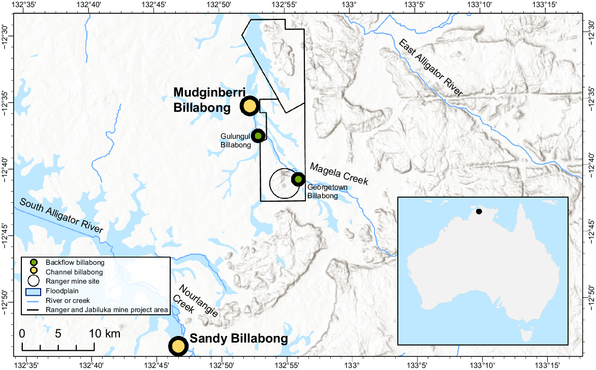
In each of the two channel billabongs, 10 replicate unbaited video cameras (GoPro, models 5–9), 5 surface and 5 benthic, were deployed along each of five transects concurrently ~5 m apart, recording for a minimum of 65 min each. In each of the backflow billabongs, six replicate unbaited video cameras were deployed along each of five transects concurrently ~10 m apart, in the benthic position, for a minimum recording of 65 min each. All cameras in channel and backflow billabongs were oriented towards the bank or habitat structure. Each 65 min of footage was analysed sequentially by personnel trained in local fish identifications, with the maximum number of individuals of each species present in any one frame (MaxN) recorded as a semi-quantitative measure of abundance.
Ethics approval
This research was conducted with approval from the Animal Ethics Committee at Charles Darwin University, Northern Territory, Australia, under project number A20005.
Conceptual flow chart of methods
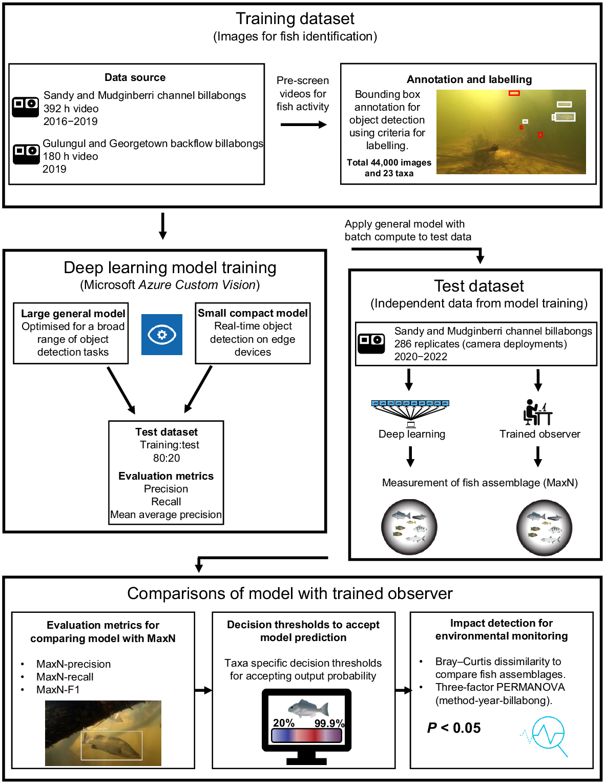
A conceptualisation of the steps used to derive a deep learning method to characterise fish assemblages from underwater videography, and to compare results to manual characterisation for monitoring, is provided in Fig. 2. Images used for fish identification and to train a CNN were annotated and labelled by trained observers from historical monitoring videos; these labelled images formed the training dataset (see ‘Training dataset’ section). Fish features used for identification, present in the training dataset, were used to train deep learning models in Azure Custom Vision (ver. 3.4, Microsoft, see https://azure.microsoft.com/en-us/products/cognitive-services/custom-vision-service/), with the models evaluated using precision, recall and mean average precision (see ‘Deep learning model training: Azure Custom Vision service’ section). An independent test dataset was derived for fish assemblage characterisation (MaxN), using both trained observers (see ‘Test dataset’ section) and deep learning (see ‘Model scoring and batch processing’ section). Comparisons between fish assemblages derived by trained observers and the general deep learning model were evaluated using MaxN-precision, MaxN-recall and MaxN-F1 (see ‘Evaluation metrics’ section), optimised with custom thresholds for accepting a model’s prediction (see ‘Optimising predictive thresholds’ section) and evaluated for monitoring potential impacts at RUM (see ‘Comparisons between fish assemblages’ section).
Training dataset
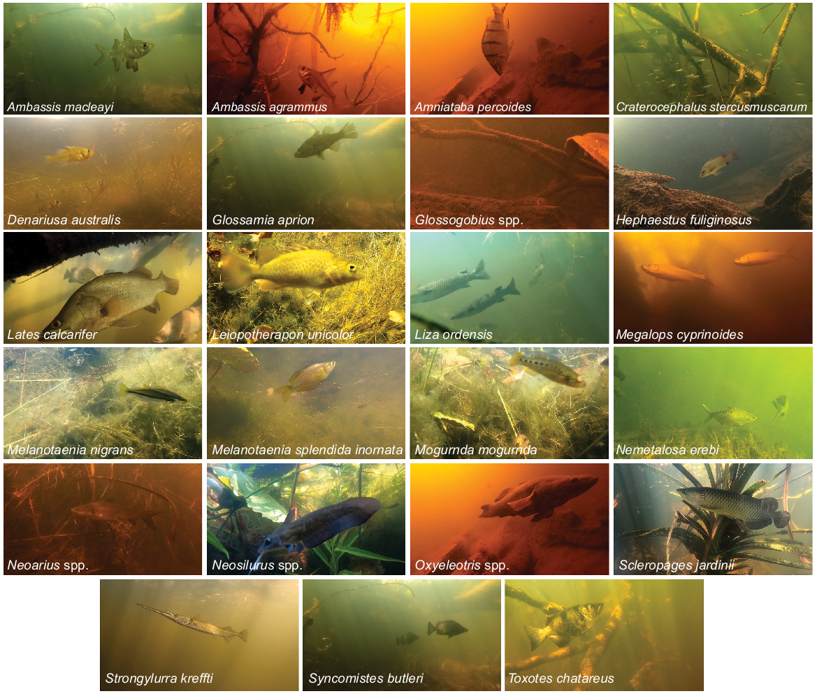
The imagery used for annotation and labelling was extracted from 392 underwater camera deployments collected from Sandy and Mudginberri billabongs between 2016 and 2019 (Supervising Scientist 2020). This imagery was supplemented with 180 camera deployments collected in July 2019 from two backflow billabongs, Gulungul and Georgetown. Videos were pre-screened for high levels of fish activity, then images were extracted from video files at a rate of 1 frame per second using customised open-source code in Python (see ‘Data availability’ section; Van Rossum and Drake 2010). This resulted in over 2 million frames for image annotation. Frames were manually examined and those without fish were discarded and those with fish present were annotated using a bounding box, then labelled by one of two experienced freshwater fish ecologists. All identifications were taken to species level where possible. It was not possible to consistently identify and separate eel-tail catfish (family Plotosidae) from within the genus Neosilurus (i.e. N. hyrtlii or N. ater), flat-head goby (family Gobiidae) from within the genus Glossogobius (i.e. G. aureus or G. giuris), gudgeons (family Eleotridae) from within the genus Oxyeleotris (i.e. O. selheimi or O. lineolate), nor distinguish fork-tailed catfish (family Ariidae) from within the genus Neoarius (i.e. N. graeffei or N. midgleyi) to species level from underwater imagery, so genus-level identification was used instead. Fig. 3 shows the 23 taxa of tropical freshwater fishes that were annotated and labelled.
Frames extracted from video footage demonstrating lowest taxonomic identification used, inter-species variability in fish morphology, differences in background and light conditions, and typical view of fish from underwater videography.
To standardise the annotation process and define ‘what makes a good label’ for a model’s intended purpose, the following criteria were developed:
Key features – fish were only annotated if key defining characteristics for the lowest taxonomic level of identification were visible in the image, such as colouration or morphology.
Orientation – fish directly facing or oriented away from the camera were not annotated, as key features are often obscured, making identification difficult.
Distance from camera and visibility – as distance between fish and the camera increases, ability to confidently identify is reduced. Deteriorating light and turbidity also make identification difficult. Annotations were only made in clear conditions satisfying these criteria.
Obstructed view – if a fish was occluded by debris, aquatic vegetation, the field of view or other fish, bounding boxes were not applied.
Geography – collection location can be used to exclude and include taxa based on their known distribution (Pusey et al. 2017) (i.e. channel v. lowland billabong, Magela v. Nourlangie catchment).
Deep learning model training: Azure Custom Vision service
The Microsoft Azure Custom Vision service was used for image annotation, labelling and model training. Azure Custom Vision is an artificial intelligence (AI) service and end-to-end platform with a GUI that enables operators without coding experience to label and train deep learning models. As such, the operator is not required to select model architectures and tuning parameters. Based on the data, the platform optimises model training and hyperparameter tuning to maximise prediction accuracy. For this study and in the Azure Custom Vision platform, an object detection project that leverages multi-taxa tagging per image was created. Two ‘domain’ models were trialled, a larger general model that is optimised for a broad range of object detection tasks, and a smaller compact model for the constraints and advantage of real-time object detection on edge devices. The compact model can be exported and so can be run locally outside of Azure Custom Vision, whereas the general model is hosted on the program’s cloud platform and is presently not publicly available. The smaller compact model results in reduced accuracy and was trained for sharing purposes only. Results from compact model training are made available in see Supplementary Table S1.
When all images that met the annotation and labelling criteria were labelled, a model was trained using the advanced training feature in Azure Custom Vision for the maximum training time allowed at the time of this study, namely 96 h of computing time. A testing dataset was parsed from the training dataset, at an 80:20 train to test split, by the Azure Custom Vision platform and used during model training to calculate evaluation metrics.
Test dataset
An independent test dataset was derived from two-hundred eighty-six 1-h video files collected from channel billabong fish monitoring (Mudginberri and Sandy) in May 2020, 2021 and 2022 (Supervising Scientist 2021). All video files contributing to the test dataset were standardised to a 1-h analysis period, after discarding the first 5 min of imagery (representing settling time); the subsequent 1 h of imagery was processed manually by trained personnel and deep learning (see ‘Model scoring and batch processing’ section for the latter) to derive MaxN for the fish assemblage.
Model scoring and batch processing
The trained general model (from ‘Deep learning model training: Azure Custom Vision service’ section) was used to predict fish taxa from all videos in the test dataset and to calculate MaxN for each taxon in the model. For each camera location, the multiple video files were processed by sequentially extracting from each file a frame from each second of video. Each frame was assessed against the general model for object detection and taxa classification. For every frame, the model recorded the number of fish taxa detected, percent confidence in its prediction, and frame and video number. For every frame with a positive fish detection, an image visualising the prediction was saved. Azure Batch, a cloud-based distributed computing platform, was used to expedite model scoring of the ~1 million frames. For this study, video frames and code were deployed and processed in parallel across 30 nodes (Microsoft Azure Data Science Virtual Machine D4s powered by a 3rd generation Intel Xeon Platinum 8370C (Ice Lake)).
Statistical analysis
The Azure Custom Vision service calculates precision, recall and mean average precision within the platform for each fish taxon and the overall model based on the validation dataset. Azure Custom Vision uses a predetermined Intersection over Union (IoU) threshold between predicted and ground truth bounding boxes and probability threshold in order for a prediction to be valid during model training. After model training, the calculation of evaluation metrics can be adjusted using custom thresholds of IoU and probability. The results presented here were calculated using 30% IoU and 80% probability thresholds. A lower 30% IoU was chosen over the standard 50% (Everingham et al. 2010) to account for high variability in fish positioning (through movement) in three-dimensional (3-D) space. These metrics, defined below, are useful for determining how the model may perform on unknown test data. As our aim was to compare results between a deep learning model and those using trained observers when calculating MaxN for a 60-min analysis period from underwater videography, we extended the usual metrics, customising and calculating MaxN-precision, MaxN-recall and MaxN-F1 scores for each taxon using the MaxN per video file. Both the Azure Custom Vision and MaxN metrics for precision, recall and (MaxN only) MaxN-F1 were calculated using the true-positive (TP), false-positive (FP) and false-negative (FN) scores. Results for Azure Custom Vision were calculated using the 20% test dataset parsed from the training data, and results for MaxN metrics were calculated using the trained observer and deep learning MaxN scores across all video files in the test dataset (n = 286 files). True-negative (TN) results were calculated and used to inform predictive thresholds (see ‘Optimising predictive thresholds’ section). A TP value was recorded when a MaxN was scored in both methods. Thus:
Precision and MaxN-precision (%) are indicators of the probability that the taxon detected is classified correctly:
Recall and MaxN-recall (%), also known as sensitivity, are indicators of the probability a model will correctly predict a taxon out of all the taxa that should be predicted:
MaxN-F1 (%), an extension of the F-measure (Chinchor 1992), is the harmonic mean of precision and recall, giving equal weight to each metric to reduce the number of false-positive and false-negatives:
Finally, mean average precision (mAP) is the average of the average precision calculated for all the taxa.
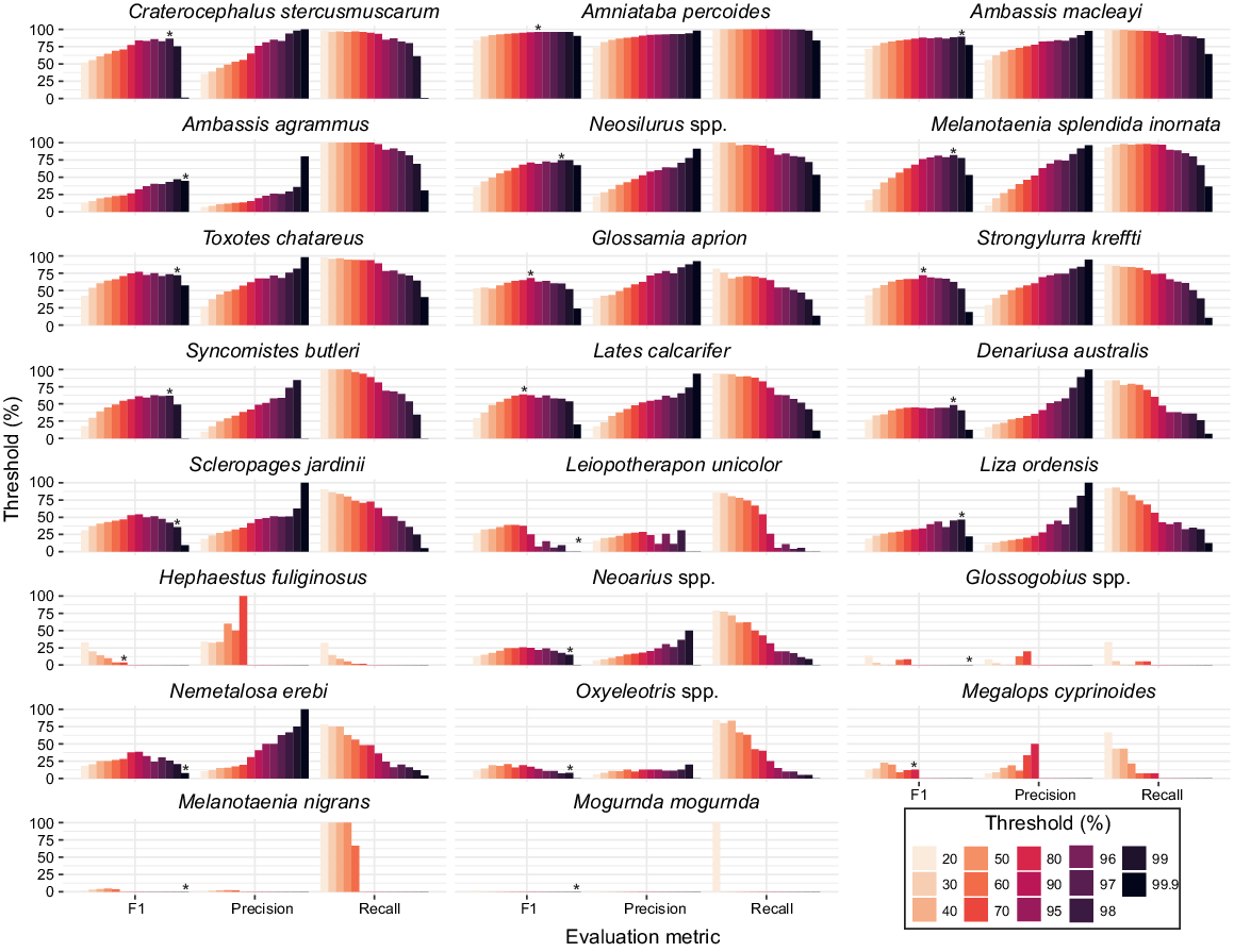
Using a threshold value on the confidence score of a model’s prediction can improve the predictive performance of a model trained with an unequal number of labels per category (Buda et al. 2018). A custom scoring threshold for accepting the model’s output probability for each fish taxon was used to calculate MaxN. Custom thresholds were derived from calculations of MaxN-precision, MaxN-recall and MaxN-F1 metrics for each taxon at thresholds between 20 and 99.9% using the MaxN per video file derived by the trained observers and deep learning. Optimum thresholds per taxon were selected from the highest MaxN-F1 score achieved. When MaxN-F1 scores were within 1–5% of each other, the threshold with higher MaxN-precision was selected. MaxN-precision was chosen over MaxN-recall on the basis that a type 2 error is preferred for biodiversity survey data; namely, missing a fish when it was actually present is a more conservative assessment than one based on scoring the presence of a fish when it was actually absent. For taxa with low MaxN-F1 scores (<50%) and low abundance, the greatest MaxN-F1 score overprioritises recall and introduces more FPs than actual observed taxa. In these instances, the TP and FP values were used to find the threshold where TP exceeded FP. MaxN-F1 scores were not reported where MaxN-precision and MaxN-recall equalled 0. Threshold data were graphed using the ggplot2 package (ver. 3.4.4, see https://CRAN.R-project.org/package=ggplot2; Wickham 2016) in the statistical analysis program R (ver. 4.0.5, R Foundation for Statistical Computing, Vienna, Austria, see https://www.r-project.org/).
All comparisons between trained observer and deep learning-derived fish assemblages were made using the test dataset. MaxN data from 10 videos at each transect were averaged for each taxon, to best represent the sampled areas. All multivariate analyses described hereon were performed using the statistical analysis program PRIMER (ver. 7, see https://www.primer-e.com/our-software/; Clarke and Gorley 2015). For calculation of similarities and the subsequent use of similarities for multivariate analyses of the assemblage, MaxN data for each fish taxon were log(x + 1) transformed. This transformation is preferred because it down-weights the abundant species, allowing moderately abundant and rarer species to have greater influence in calculations of community structure (Clarke and Gorley 2006). Bray–Curtis dissimilarity was used to compare fish assemblages within and between each billabong at time of sampling. Differences between methods (trained observer and deep learning), billabongs and years were tested using a three-way crossed PERMANOVA design, setting ‘billabong’ and ‘method’ as fixed factors and ‘year’ as a random factor. Permutation of residuals under a reduced model was performed with 9999 permutations, and Monte–Carlo (MC) tests to account for factors, billabong and method, which had low numbers of unique permutations to reasonably accept the P-value (Anderson 2017). The Bray–Curtis dissimilarity matrix was visualised in ordination space using principal coordinate ordination (PCO), which is a direct projection of the dissimilarity matrix. Fish taxa deemed to influence the distribution of fish assemblages in the ordination space were based on Pearson correlations greater than 0.2, with these taxa and vectors overlayed on the PCO plot. The length and direction of vector lines indicate the strength of influence on sample similarity. Species contribution to sample similarity (SIMPER) was calculated on all trained observer-derived fish assemblage data between 2016 and 2022, to determine the percent contribution of each taxon to the overall assemblage, and hence the influence of taxa included in the model.
Results
Deep learning model training results
A total of 44,112 images representing 23 fish taxa were annotated with 82,904 bounding boxes and labelled (Table 1). mAP, precision and recall for overall model performance were 83.6, 81.3 and 89.1% respectively (Table 1). Of the 23 taxa used for model training, 11 taxa recorded average precision (AP) >90%, half of which had >8000 annotations per taxa. The remaining 12 taxa recorded AP between 29 and 87% with total number of annotations ranging between 20 and 3033. Banded grunter (Amniataba percoides) had the highest AP (96.3%) and Black bream (Hephaestus fuliginosus) had the lowest AP (29.0%).
| Taxa name | Number of annotations | Number of images with annotations | Precision (%) | Recall (%) | AP (%) | SIMPER (%) | |
|---|---|---|---|---|---|---|---|
| All taxa in model | 82,904 | 51,737 | 81.3 | 89.1 | 83.6 A | 100.0 | |
| Ambassis agrammus | 8947 | 5565 | 81.4 | 87.1 | 90.8 | 0.7 | |
| Ambassis macleayi | 16,105 | 8578 | 84.1 | 85.6 | 92.6 | 17.2 | |
| Amniataba percoides | 12,199 | 8150 | 87.2 | 94.6 | 96.3 | 17.0 | |
| Craterocephalus stercusmuscarum | 3033 | 1388 | 58.2 | 86.3 | 81.9 | 28.7 | |
| Denariusa australis | 892 | 719 | 76.1 | 66.7 | 75.3 | 0.9 | |
| Glossamia aprion | 1551 | 1401 | 82.2 | 85.6 | 90.0 | 3.8 | |
| Glossogobius spp. | 20 | 20 | 100.0 | 25.0 | 78.1 | 0.6 | |
| Hephaestus fuliginosus | 35 | 35 | 0.0 | 0.0 | 29.0 | 1.0 | |
| Lates calcarifer | 430 | 404 | 79.3 | 73.0 | 80.3 | 2.1 | |
| Leiopotherapon unicolor | 150 | 147 | 75.0 | 50.0 | 72.1 | 0.8 | |
| Liza ordensis | 155 | 117 | 83.8 | 91.2 | 95.6 | 0.5 | |
| Megalops cyprinoides | 47 | 32 | 100.0 | 11.1 | 67.2 | 0.1 | |
| Melanotaenia nigrans | 9479 | 4182 | 75.5 | 88.4 | 90.4 | 0.0 | |
| Melanotaenia splendida inornata | 14,824 | 10,358 | 81.6 | 92.1 | 94.1 | 6.1 | |
| Mogurnda mogurnda | 83 | 83 | 100.0 | 64.7 | 76.1 | 0.0 | |
| Nemetalosa erebi | 151 | 141 | 96.3 | 81.3 | 84.0 | 0.5 | |
| Neoarius spp. | 250 | 245 | 85.7 | 58.8 | 79.5 | 0.6 | |
| Neosilurus spp. | 11,882 | 7706 | 82.7 | 93.0 | 95.3 | 8.5 | |
| Oxyeleotris spp. | 83 | 83 | 100.0 | 58.8 | 87.0 | 0.1 | |
| Scleropages jardinii | 167 | 164 | 82.4 | 82.4 | 87.0 | 0.7 | |
| Strongylura kreffti | 596 | 554 | 97.1 | 83.6 | 94.7 | 2.9 | |
| Syncomistes butleri | 882 | 822 | 82.4 | 82.9 | 90.3 | 2.6 | |
| Toxotes chatareus | 943 | 840 | 93.2 | 93.7 | 95.8 | 4.8 |
Optimising decision thresholds
Thresholds ranged between 70 and 99.9% for recording a MaxN (Fig. 4), whereas these varied across fish taxa, some trends were evident. For taxa low in abundance in test videos, MaxN estimates had greater uncertainty because of poor model detectability. This is evident in the five taxa (Glossogobius spp., Leiopotherapon unicolor, Melanotaenia nigrans, Mogurnda mogurnda and Oxyeleotris spp.) that did not record a MaxN. These taxa were constrained at 99.9% threshold and individually contributed <1% to fish assemblage composition (see Supplementary Table S2). Although lower thresholds would have recorded a MaxN, as evident in the higher MaxN-recall at decreasing thresholds (Fig. 4), the MaxN-precision remains low (<30%). This would result in more FP than TP detections, thus increasing the chance of type 1 error. This logic was applied to other low abundant taxa such as Scleropagaes jardinii and Nemetalosa erebi where the highest MaxN-F1 resulted in similar counts of FP and TP detection. A 70% threshold was allocated to one taxon, H. fulifinosus, the only fish that recorded 100% MaxN-Precision at a threshold below 99.9%. For all taxa, the greatest MaxN-recall and lowest MaxN-precision was calculated at 20% threshold. The highest MaxN-F1 score of 96.1% was calculated for A. percoides, with a threshold of 95%, where the model and trained observer MaxN matched 100% of the time. Taxa with a high number of annotations (>2000) were allocated a high threshold (≥95%). The most abundant fish in videos and with the greatest number of annotations were Ambassis macleayi, A. percoides and Craterocephalus stercusmuscarum, which had respectively 16,105, 12,199 and 3033 annotations and thresholds between 95 and 98%. From the assemblage derived with optimal thresholds, the mean MaxN-F1, MaxN-precision and MaxN-recall scores across 286 videos were 54.4, 76.5 and 56.6% respectively (see Table S2).
Trained observer v. deep learning for monitoring at RUM
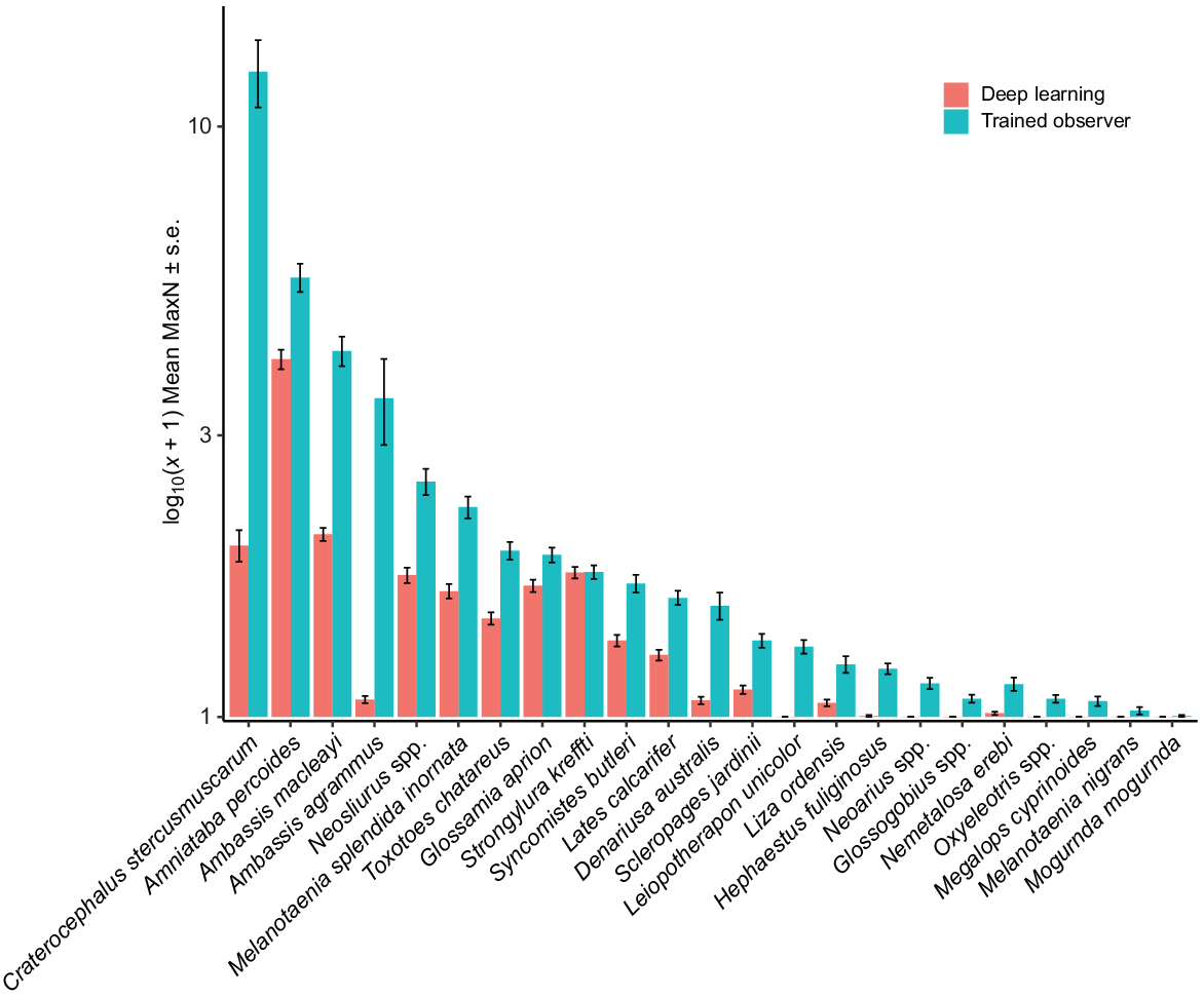
PERMANOVA results showed significant differences between methods (deep learning and trained observer) (Pseudo-F = 14.977, P(MC) = 0.0002), billabongs (Sandy and Mudginberri) (Pseudo-F = 3.6648, P(MC) = 0.0244) and among the years (Year) (Pseudo-F = 5.6761, P(MC) = 0.0001) being compared. PCO of axes 1 and 2, cumulatively representing 55% of the variation in Bray–Curtis similarity (Fig. 5), showed clear separation of samples by method. This is evident across the x-axis and is primarily due to a larger, trained-observer-derived MaxN for abundant and, often schooling, taxa (e.g. C. stercusmuscarum, A. macleayi, Neosilurus spp. and Melanotaenia splendida inornata) (Fig. 6). The interactions between method and year (Pseudo-F = 2.7674, P(MC) = 0.0011) and billabong and year (Pseudo-F = 3.6875, P(MC) = 0.0002) were also significant, indicating that difference between methods and the difference between billabongs varied across years.
Principal coordinate ordination (PCO) of fish assemblages (mean MaxN per transect) at Mudginberri and Sandy billabongs derived using deep learning and trained observers in 2020, 2021 and 2022 (n = 10). Transect numbers are denoted above each symbol.
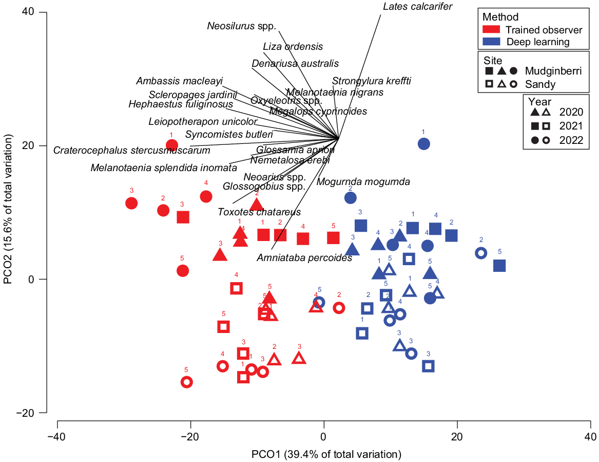
There was no significant difference for the remaining factors and their respective interactions (method × billabong and method × billabong × year, see Supplementary Table S3). Although differences in MaxN were observed between methods, the non-significant interaction between method × billabong × year indicates the distribution of taxa and their relative abundances in samples determined by each method reflect the same relative changes between billabongs over 3 years. This is shown in the PCO where the assemblages for each billabong and year are otherwise arranged in a similar pattern on their respective sides of the ordination, namely strong concordance between methods on the y-axis of the PCO plot for separation of billabong and year (Fig. 6).
Discussion
Deep learning for fish monitoring
Deep learning is a valuable tool for automating the measurement of tropical freshwater fish assemblages, and when used in a real-world monitoring scenario such as the present study, produced results that approached those of trained observers. To the best of our knowledge, the training dataset we developed is the largest and most diverse generated for tropical freshwater fish worldwide, and was produced using a low-code, user-friendly tool. Deep learning was able to effectively detect spatio-temporal patterns in fish assemblages, expanding enormously future applications in the assessment and measurement of fish communities. In particular, with automated fish counting systems, environmental managers can increase the number of replicates used both temporally and spatially to sample an area and generate more detailed ecological datasets. Additionally, new measures of abundance can be explored such as MeanCount – the mean number of fish detected in a series of frames over an analysis period (Schobernd et al. 2014) – due to the ease of collecting fish abundance data for any time interval of video.
If deep learning and automated systems for processing underwater fish videography are to supplement or replace conventional traditional manual methods that rely on high levels of human interaction, deep learning must provide comparable ecological information. Tropical freshwater fish assemblages are dependent upon a range of ecological processes, from the flood pulse concept (Junk 1999) to changes in habitat structure (Buckle and Humphrey 2013). This study aimed to determine if assemblages measured by deep learning capture the same trends and variation through space and time as data derived from trained observers. Our results indicate significant differences between deep learning and trained observers for deriving MaxN of multiple fish taxa in underwater video. A significant difference between methods is not unexpected because of the complexity of fish detection and classification in underwater videography and was evident in the separation of samples in multivariate space, in particular, across the x-axis in the PCO (Fig. 5). By contrast, there was no significant interaction in method, billabong and year from PERMANOVA testing. That is, the distribution of taxa and their relative abundances in samples determined by deep learning and trained observers reflect the same relative changes between Mudginberri and Sandy billabongs over a 3-year period. The limitations presented by deep learning were primarily lower average species-wise MaxN measures for some taxa and inability to detect rarer taxa because of lack of specific types of training data, as described below. Regardless, we have demonstrated the use of deep learning in a real-world fish monitoring program, and present results that show where efforts to improve the deep learning model can be targeted to close the gap between trained observers and deep learning.
Our study’s overall mAP of 83.6% was comparable to other multi-species fish object detection F1 scores from test data of 79.8% for 14 taxa (Jalal et al. 2020) and 83.3% for 4 taxa (Knausgård et al. 2022). However, these studies used a two-staged detector approach where object detection models were trained on one category, ‘fish’, then detections of fish were assessed against an image classification model. Our results suggest that similar performance can be achieved on novel test data using a single-stage multi-taxa object detection model. We present the first mean per video MaxN-F1 score between trained observers and deep learning of 54.4% for tropical freshwater fish. On average, deep learning’s estimate of fish abundance was approximately half that of a trained observer. This difference in accuracy between the model’s training metrics (e.g. 83.6% mAP) and its performance in real-world situations (e.g. 54.4% MaxN-F1) emphasises the need to validate a model against the specific analytical routines it will be used for in practice. It also highlights the importance of understanding any limitations of the model, such as underestimation of abundance, that may not have been apparent in the standard training, validation and testing process.
Thresholds
We present an approach to define the optimal threshold for deriving MaxN per taxon. This was highly effective for taxa with lower volumes of training data and was necessary to reduce the number of FPs. Thresholds for accepting the model’s output probability were highly variable among taxa. Given the differences in training data size and the subsequent precision, recall and mAP results for each taxon from model training, the range in thresholds between 70 and 99.9% were expected and consistent with multi-taxa fish classification thresholds derived elsewhere (Villon et al. 2020). Constraining the prediction thresholds for each taxon improved the model’s overall performance. Our results indicate the importance of deriving taxon-specific thresholds and highlight the implications and limitations of using one threshold for accepting multi-taxa deep learning model predictions. For example, if 95% acceptance criteria were applied to all model predictions taxa such as A. percoides would record the optimum balance of precision and recall. By contrast, taxa such as Ambassis agrammus would sacrifice precision for recall and record 143 FP predictions at 95% threshold compared to 3 FP predictions at 99.9% threshold, which was calculated as the optimum balance between precision and recall.
Deep learning and MaxN
The fish monitoring program designed for impact detection at RUM is based on an indicator approach that measures a subset of ‘common’ species in the knowledge that no single method can capture all species, and all monitoring methods have their inherent biases. Analyses of fish assemblage data using Bray–Curtis similarity places greater emphasis on the numerically dominant taxa and less weight on uncommon taxa. Overall, when the deep learning model was applied to test data to derive MaxN for real-world monitoring of fish, the evaluation metrics were lower compared to those derived during model training with Azure Custom Vision. As the model results were optimised for precision when selecting thresholds, and consequently the MaxN-F1, this result was expected and is commonly encountered when applying deep learning to real world scenarios. For the most abundant fish, A. macleayi, A. percoides and C. stercusmuscarum, the MaxN-F1 score was similar to or greater than the model’s mAP. This may be explained by the way MaxN is used as a measure of abundance. MaxN has become the common metric used for quantifying fish abundance from underwater video (Cappo et al. 2001; Whitmarsh et al. 2017). Although it is a conservative estimate of abundance (Campbell et al. 2015), MaxN has proved its capability in detecting spatio-temporal variability in fish assemblages and ecological nuances in fish data (Whitmarsh et al. 2017).
For deep learning to be successfully used for MaxN estimates, the model must be able to confidently identify one frame out of the 3600 possible frames in a 60-min analysis period for which the maximum number of fish of a particular taxon are present. The MaxN may occur multiple times in a 60-min video and the model may perform differently based on how the fish are displayed in those frames. If the MaxN was recorded in a frame where most fish were deep in the field of view or were obscured by vegetation, then the model may not detect all individuals present in the frame and will underestimate MaxN. Conversely, if all fish are clearly in view, and therefore representative of the training data, it is more likely the model will confidently return the correct MaxN. In this study, we observed consistently lower measures of MaxN for abundant schooling taxa presenting deep in the field of view or obscured by vegetation. There is the potential that lower measures of an already conservative abundance estimate may reduce the ability to detect changes in fish assemblages for monitoring purposes. For monitoring at RUM, a number of numerically dominant fish species have greater abundances in the exposed (Mudginberri) site than the reference (Nourlangie) site (e.g. M. splendida inornata, C. stercusmuscarum and A. macleayi). Underestimates of these numerically dominant taxa increase the possibility of a type 1 error because of the method’s artefact in the down-weighting of their abundances in the exposed site. Although the distribution of taxa and their relative abundances in samples determined by deep learning and trained observers reflect the same relative changes between Mudginberri and Sandy (non-significant three-way PERMANOVA interaction), significant differences between methods were observed using PERMANOVA. The implications of such artefacts are yet to be assessed. Assessment would entail statistical comparisons of multi-year data derived from deep learning and trained observers, with possible data manipulation to mimic impact upon numerically dominant taxa. In parallel, improved deep learning detection of schooling numerical dominants is also required.
Currently, one of the greatest challenges with deep learning for fisheries estimates is access to high quality, annotated and labelled training data that cover all taxa expected in a test environment (Villon et al. 2022). While such datasets are desirable, considerable efforts may be required to curate and achieve high performance across all taxa for monitoring purposes, particularly all uncommon species. As our aim was to develop a model that could accurately detect the MaxN for each taxon in a 60-min analysis period, several considerations were made around annotation and labelling to optimise performance. Bounding box annotations were chosen over polygons because of the speed and efficiency for generation of a bounding box dataset. Polygons are preferred when the objects of interest are often overlapping or close to each other and where use of bounding boxes would result in high degrees of overlap. However, polygons require significantly more resources and can cost twice as much as bounding boxes to annotate (Mullen et al. 2019). Fisheries monitoring in marine ecosystems using videography often use baits to attract fish to the camera, resulting in imagery with overlapping fish (Ditria et al. 2021; Harvey et al. 2021). For videography in freshwater ecosystems that do not use baited bags, the density of fish observed per frame can be lower because of the lack of an attractant, resulting in more frames with individual fish spread across the field of view rather than overlapping. In these scenarios the less resource-intensive bounding boxes are adequate.
Training data
Generating a training dataset from video with fish moving in 3-D space can be a significant challenge for deep learning in terms of distinguishing all taxa and their identifying features (Jalal et al. 2020). Precision, recall and overall accuracy increase logarithmically with increasing number of images when training deep learning models (Shahinfar et al. 2020). Therefore, to maintain high taxa detection accuracy across multiple species classes, a neural network must be trained with enough labelled images across a range of poses, orientations, lighting conditions and body size when moving through the field of view, to return a uniform and consistently accurate score when making inferences on unseen footage. Although the dataset generated in this study has reasonably few images of low-abundant taxa, we were still able to build an understanding and present results on taxa-specific, deep learning performance. Our results indicate that taxa that are comparatively unique, such as A. percoides with distinct black and white bands across its body (Fig. 3) and low morphological variation between sexes, reproductive cycle and life stage (Bishop et al. 2001), could achieve a high MaxN-F1 score (96%) on a test set when trained with >12,000 annotations. Conversely, for a similar number of annotations for taxa with high intra-species variation, such as M. splendida inornata, there was reduced accuracy on a test set (81%) and a higher number of FP detections. Factors such as changes in colour during reproductive cycle (Crowley and Ivantsoff 1982) and a preference for habitat near the surface of the water column with associated influences of poor light and water clarity introduce additional noise into the imagery that must be learnt.
Conservation and biodiversity assessment
Missing taxa from a model prediction has implications when monitoring metrics rely upon taxa richness in impact or conservation and biodiversity assessments. This includes consideration of taxon-specific migration responses to the magnitude of wet season rainfall, which may see the effect of missing taxa exacerbated in years where movement of typically low-abundant fish in channel billabongs is enhanced by antecedent wet season productivity (Crook et al. 2020, 2023). In other instances, usually uncommon taxa may dominate in stochastic fashion at decadal intervals. Until training datasets are improved, deep learning as a monitoring tool should be used with these considerations in mind. To apply this learning to conservation and biodiversity assessments, it is important to prioritise the generation of training data for uncommon or rare species. Until such data is available potential procedures during QA/QC of biodiversity data may mitigate the effect of low abundant taxa, such as visual interrogation of model predictions to confirm the correct taxa are assigned for MaxN measures, which is more time effective than traditional video processing methods. Furthermore, where there is an overlap in taxa similarity, for example L. unicolor and juvenile Lates calcarifer can be mistaken because of their similar body shape, the model may incorrectly assign taxa into the similar category (Vuttipittayamongkol et al. 2021). This will appear as an overestimate in abundance and may be obvious in assemblage composition data, warranting further investigation and access to additional training data to improve the model. The low-abundant taxa were also noted by trained observers as having morphological overlap to each other. For example, L. ordensis, M. cyprinoides and N. erebi are all taxa that often appear elongated when swimming through the water and have similar silver-coloured bodies (Fig. 3). As the impact of training data imbalance on model performance is influenced by the presence of category overlap (Vuttipittayamongkol et al. 2021), other approaches may be required to confidently detect such taxa until training data can be improved. Although not tested here, some promising methods to improve training data imbalance include data augmentation with generative adversarial networks used to generate ‘fake’ data and balance the dataset (Ali-Gombe et al. 2019), and ensemble modelling where multiple models are trained for subsets of the taxa and test imagery is scored against all models. With the latter, significant increases in computational requirements are expected.
Although this study did not focus on optimising model performance through different data augmentations, downsampling or upsampling, by making the full annotated and labelled dataset publicly available, further research on the implications of imbalance for fish taxa detection is possible.
Taxa-specific response to deep learning
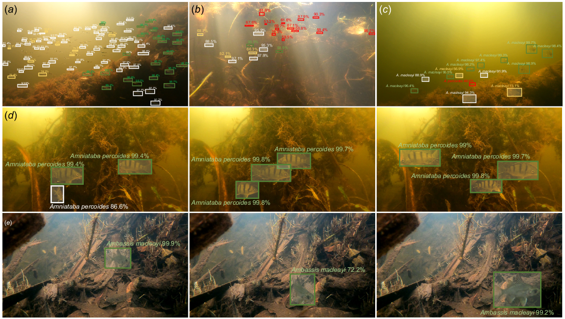
This study identified that MaxN abundance was lower for the deep learning method than for trained observers for most fish species. This was most evident in schooling taxa such as A. macleayi, C. stercusmuscarum, M. splendida inornata and Neosilurus spp., which had MaxN abundance two or more times greater for trained observers (Fig. 6). One possible explanation for this observation is that schools are often present at a range of distances relative to the camera, and individuals in the background of the image often returned confidence probabilities that did not meet the threshold set for that fish. In comparison, individuals closer to the camera lens, in clear focus and with key identifying features in view, were confidently predicted and recorded a MaxN value. Additionally, when multiple fish in view are orientated differently towards the camera, predictive performance changes. This is observed for A. percoides in Fig. 7d where, in the first (left) frame, one fish moves away from a lateral view and the bandings that distinguish this species become obscured. When facing directly toward the camera, confidence drops to 86.6% indicating that for this frame it would be below the prediction threshold of 95% and not be included in a MaxN estimate. However, because the sequence of frames will eventually show all three fish in a lateral, readily identifiable view (central and right frames of Fig. 7d), the prediction will exceed the threshold of 95% for accepting model confidence probability, and the MaxN of 3 will be scored. The same holds for A. macleayi; among other features, ichthyologists use the dark patch, often appearing as a black dot, positioned at the base of the pectoral fin for species identification. This feature separates this species from other ambassid species (Pusey et al. 2004). As the fish moves to show a lateral view with the black patch in combination with a clearer view of the body structure, the confidence probability increases from 72.2% (central frame, Fig. 7e) to 99.2% or greater (left and right frames, Fig. 7e).
Spatio-temporal variation in deep learning predictions of fish. Bounding boxes represent predictions made above the threshold for acceptance (green), below the threshold but equal to or greater than 80% (white), less than 80% (yellow) and FP predictions (red). Variation in predictions of schools deep in the field of view are depicted for C. stercusmuscarum (a, b), A. macleayi (c) and A. percoides (d). Changes in prediction confidence as fish move in 3-D space are depicted in a sequence of frames for A. percoides and A. macleayi (e).
Our results suggest that the model is learning the morphological features ichthyologists use for taxonomic identification of fish, and that this form of interpretation of deep learning predictions, where ecology and data science intersect, is critical to inform how deep learning is best applied to automating fish monitoring and where effort is optimised on improving performance. For example, to improve the accuracy of M. splendida inornata described previously, the collection of training data can focus on the morphological variants that are unequal within the distribution of samples. One approach is that taxa can be separated into multiple categories if the intraspecies variation is divergent enough to warrant such a split. We have identified taxa with the same number of annotations that were learnt by deep learning at different precisions. This may be because some taxa are more difficult to learn because of their complex morphology, inter-species similarity, intra-species variation and behaviour that can influence the ability to identify taxa across test scenarios. Notwithstanding and despite the underestimation of MaxN using deep learning, we provide evidence that the approach preserved the relative fish assemblage differences between both billabongs and among years. In these respects, results are similar to those derived by a trained observer when making comparisons between assemblages.
Conclusions
Deep learning applied to fish identification is a useful method for automating the analysis of large volumes of underwater videography. When making predictions on test imagery for object detection of fish, taxa-specific thresholds were necessary to reduce the number of FP detections and ensure the model could be used dynamically for unequal classes. Significant differences were found between deep learning and trained observers for deriving MaxN of multiple fish taxa in underwater video, driven primarily by underestimates of MaxN by deep learning for numerically dominant fish. When methods were compared for monitoring impact detection in a real-world scenario (RUM) there was no significant interaction in method, billabong and year from PERMANOVA testing. This suggests that for both methods the distribution of taxa and their relative abundances reflect the same relative changes between control and exposed billabongs over a 3-year period. However, the implications of method differences need to be considered for impact detection and additional work is required to better characterise and quantify small-growing schooling fish species. Interpretation of deep learning performance is best made through analysis of evaluation metrics, with an ecological and data science lens, that aims to improve future environmental monitoring.
Data availability
The training data are available on Zenodo (https://zenodo.org/record/7250921). Code used for this project is available at https://github.com/ajansenn/KakaduFishAI.
Acknowledgements
The authors acknowledge the Mirrar Traditional Owners past, present and emerging, from the land that this research was undertaken in Kakadu National Park. We thank Dave Walden who assisted in generating the training dataset for this project and Valeriia Savenko for assistance using the compact model in Azure.
References
Ali-Gombe A, Elyan E, Jayne C (2019) Multiple fake classes GAN for data augmentation in face image dataset. In ‘2019 International Joint Conference on Neural Networks (IJCNN)’, 14–19 July 2019, Budapest, Hungary. Paper N-20152. (IEEE) doi:10.1109/IJCNN.2019.8851953
Almeida JS (2002) Predictive non-linear modeling of complex data by artificial neural networks. Current Opinion in Biotechnology 13(1), 72-76.
| Crossref | Google Scholar | PubMed |
Alshdaifat NFF, Talib AZ, Osman MA (2020) Improved deep learning framework for fish segmentation in underwater videos. Ecological Informatics 59, 101121.
| Crossref | Google Scholar |
Australian Institute of Marine Science, University of Western Australia, Curtin University (2020) OzFish dataset – machine learning dataset for baited remote underwater video stations. Available at https://apps.aims.gov.au/metadata/view/38c829d4-6b6d-44a1-9476-f9b0955ce0b8 [Dataset, verified 1 February 2020]
Bishop KA, Pidgeon RWJ, Walden DJ (1995) Studies on fish movement dynamics in a tropical floodplain river: prerequisites for a procedure to monitor the impacts of mining. Australian Journal of Ecology 20(1), 81-107.
| Crossref | Google Scholar |
Buckle D, Humphrey C (2013) Monitoring using fish community structure. In ‘eriss research summary 2011–2012’. (Eds RA van Dam, A Webb, SM Parker) Supervising Scientist report 204, pp. 97–101. (Supervising Scientist, Australian Government Department of Sustainability, Environment, Water, Population and Communities: Darwin, NT, Australia) Available at https://www.dcceew.gov.au/sites/default/files/documents/ssr204.pdf
Buda M, Maki A, Mazurowski MA (2018) A systematic study of the class imbalance problem in convolutional neural networks. Neural Networks 106, 249-259.
| Crossref | Google Scholar | PubMed |
Bush A, Compson ZG, Monk WA, Porter TM, Steeves R, Emilson E, Gagne N, Hajibabaei M, Roy M, Baird D (2019) Studying ecosystems with DNA metabarcoding: lessons from biomonitoring of aquatic macroinvertebrates. Frontiers in Ecology and Evolution 7, 434.
| Crossref | Google Scholar |
Campbell MD, Pollack AG, Gledhill CT, Switzer TS, DeVries DA (2015) Comparison of relative abundance indices calculated from two methods of generating video count data. Fisheries Research 170, 125-133.
| Crossref | Google Scholar |
Cappo M, Speare P, Wassenberg T, Harvey E, Rees M, Heyward A, Pitcher R (2001) The use of baited remote underwater video stations (BRUVS) to survey demersal fish stocks – how deep and meaningful. In ‘Video sensing of the size and abundance of target and non-target fauna in Australian fisheries: a national workshop. FRDC Proiect 2000/187’, 4–7 September 2000, Rottnest Island, WA, Australia. (Eds E Harvey, M Cappo) pp. 63–71. (Fisheries Research Development Corporation: Canberra, ACT, Australia) Available at https://www.frdc.com.au/sites/default/files/products/2000-187-DLD.pdf
Chinchor N (1992) Muc-4 evaluation metrics. In ‘Proceedings of the Fourth Message Understanding Conference’, 16–18 June 1992, McLean, VA, USA. pp. 22–29’. (Morgan Kaufmann) Available at https://aclanthology.org/M92-1002.pdf
Connolly RM, Fairclough DV, Jinks EL, Ditria EM, Jackson G, Lopez-Marcano S, Olds AD, Jinks KI (2021) Improved accuracy for automated counting of a fish in baited underwater videos for stock assessment. Frontiers in Marine Science 8, 658135.
| Crossref | Google Scholar |
Crook DA, Buckle DJ, Morrongiello JR, Allsop QA, Baldwin W, Saunders TM, Douglas MM (2020) Tracking the resource pulse: movement responses of fish to dynamic floodplain habitat in a tropical river. Journal of Animal Ecology 89(3), 795-807.
| Crossref | Google Scholar | PubMed |
Crook DA, Wedd D, Adair BJ, Mooney TJ, Harford AJ, Humphrey CL, Morrongiello JR, King AJ (2023) Evaluation and refinement of a fish movement model for a tropical australian stream subject to mine contaminant egress. Environmental Biology of Fishes 106, 469-490.
| Crossref | Google Scholar |
Crowley LELM, Ivantsoff W (1982) Reproduction and early stages of development in two species of Australian rainbowfishes, Melanotaenia nigrans (richardson) and Melanotaenia splendida inornata (Castelnau). Australian Zoologist 21(1), 85-95.
| Crossref | Google Scholar |
Dafforn KA, Johnston EL, Ferguson A, Humphrey CL, Monk W, Nichols SJ, Simpson SL, Tulbure MG, Baird DJ (2016) Big data opportunities and challenges for assessing multiple stressors across scales in aquatic ecosystems. Marine and Freshwater Research 67(4), 393-413.
| Crossref | Google Scholar |
Del Sole A (2018) Introducing Microsoft cognitive services. In ‘Microsoft Computer Vision APIs distilled: getting started with cognitive services’. pp. 1–4. (Apress: Berkeley, CA, USA) doi:10.1007/978-1-4842-3342-9_1
Ditria EM, Lopez-Marcano S, Sievers M, Jinks EL, Brown CJ, Connolly RM (2020) Automating the analysis of fish abundance using object detection: optimizing animal ecology with deep learning. Frontiers in Marine Science 7, 429.
| Crossref | Google Scholar |
Ditria EM, Connolly RM, Jinks EL, Lopez-Marcano S (2021) Annotated video footage for automated identification and counting of fish in unconstrained seagrass habitats. Frontiers in Marine Science 8, 629485.
| Crossref | Google Scholar |
Everingham M, Van Gool L, Williams CKI, Winn J, Zisserman A (2010) The pascal visual object classes (VOC) challenge. International Journal of Computer Vision 88(2), 303-338.
| Crossref | Google Scholar |
Follana-Berná G, Palmer M, Lekanda-Guarrotxena A, Grau A, Arechavala-Lopez P (2020) Fish density estimation using unbaited cameras: accounting for environmental-dependent detectability. Journal of Experimental Marine Biology and Ecology 527, 151376.
| Crossref | Google Scholar |
Garcia R, Prados R, Quintana J, Tempelaar A, Gracias N, Rosen S, Vågstøl H, Løvall K (2020) Automatic segmentation of fish using deep learning with application to fish size measurement. ICES Journal of Marine Science 77(4), 1354-1366.
| Crossref | Google Scholar |
Hannweg B, Marr SM, Bloy LE, Weyl OLF (2020) Using action cameras to estimate the abundance and habitat use of threatened fish in clear headwater streams. African Journal of Aquatic Science 45, 372-377.
| Crossref | Google Scholar |
Harvey ES, McLean DL, Goetze JS, Saunders BJ, Langlois TJ, Monk J, Barrett N, Wilson SK, Holmes TH, Ierodiaconou D, Jordan AR, Meekan MG, Malcolm HA, Heupel MR, Harasti D, Huveneers C, Knott NA, Fairclough DV, Currey-Randall LM, Travers MJ, Radford BT, Rees MJ, Speed CW, Wakefield CB, Cappo M, Newman SJ (2021) The BRUVS workshop – an Australia-wide synthesis of baited remote underwater video data to answer broad-scale ecological questions about fish, sharks and rays. Marine Policy 127, 104430.
| Crossref | Google Scholar |
Hebert PDN, Cywinska A, Ball SL, deWaard JR (2003) Biological identifications through DNA barcodes. Proceedings of the Royal Society of London – B. Biological Sciences 270(1512), 313-321.
| Crossref | Google Scholar |
Humphrey CL, Dostine PL (1994) Development of biological monitoring programs to detect mining-waste impacts upon aquatic ecosystems of the alligator rivers region, northern territory, Australia. Internationale Vereinigung für Theoretische und Angewandte Limnologie: Mitteilungen 24(1), 293-314.
| Google Scholar |
Humphrey CL, Bishop KA, Brown VM (1990) Use of biological monitoring in the assessment of effects of mining wastes on aquatic ecosystems of the alligator rivers region, tropical northern Australia. Environmental Monitoring and Assessment 14(2-3), 139-181.
| Crossref | Google Scholar | PubMed |
Humphrey CL, Bishop KA, Dostine PL (2016) Vulnerability of fish and macroinvertebrates to key threats in streams of the Kakadu region, northern Australia: assemblage dynamics, existing assessments and knowledge needs. Marine and Freshwater Research 69(7), 1092-1109.
| Crossref | Google Scholar |
Jalal A, Salman A, Mian A, Shortis M, Shafait F (2020) Fish detection and species classification in underwater environments using deep learning with temporal information. Ecological Informatics 57, 101088.
| Crossref | Google Scholar |
Junk WJ (1999) The flood pulse concept of large rivers: learning from the tropics. River Systems 11, 261-280.
| Crossref | Google Scholar |
Khan S, Rahmani H, Shah SAA, Bennamoun M (2018) A guide to convolutional neural networks for computer vision. Synthesis Lectures on Computer Vision 8(1), 1-207.
| Crossref | Google Scholar |
King AJ, George A, Buckle DJ, Novak PA, Fulton CJ (2018) Efficacy of remote underwater video cameras for monitoring tropical wetland fishes. Hydrobiologia 807(1), 145-164.
| Crossref | Google Scholar |
Knausgård KM, Wiklund A, Sørdalen TK, Halvorsen KT, Kleiven AR, Jiao L, Goodwin M (2022) Temperate fish detection and classification: a deep learning based approach. Applied Intelligence 52, 6988-7001.
| Crossref | Google Scholar |
Liberty E, Karnin Z, Xiang B, Rouesnel L, Coskun B, Nallapati R, Delgado J, Sadoughi A, Astashonok Y, Das P, et al. (2020) Elastic machine learning algorithms in Amazon SageMaker. In ‘SIGMOD’20: Proceedings of the 2020 ACM SIGMOD International Conference on Management of Data’, 14–19 June 2020, Portland, OR, USA. (Eds D Maier, R Pottinger, AH Doan, W-C Tan, A Alawini, HQ Ngo) pp. 731–737. (Association for Computing Machinery: New York, NY, USA) Available at https://ssc.io/pdf/modin711s.pdf
Mullen JF Jr, Tanner FR, Sallee PA (2019) Comparing the effects of annotation type on machine learning detection performance. In ‘2019 IEEE/CVF Conference on Computer Vision and Pattern Recognition Workshops (CVPRW)’, 16–17 June 2019, Long Beach, CA, USA. pp. 855–861. (IEEE) doi:10.1109/CVPRW.2019.00114
Nichols JD, Williams BK (2006) Monitoring for conservation. Trends in Ecology & Evolution 21(12), 668-673.
| Crossref | Google Scholar | PubMed |
Norouzzadeh MS, Nguyen A, Kosmala M, Swanson A, Palmer MS, Packer C, Clune J (2018) Automatically identifying, counting, and describing wild animals in camera-trap images with deep learning. Proceedings of the National Academy of Sciences 115(25), E5716-E5725.
| Google Scholar |
Pudaruth S, Nazurally N, Appadoo C, Kishnah S, Vinayaganidhi M, Mohammoodally I, Ally YA, Chady F (2020) Superfish: a mobile application for fish species recognition using image processing techniques and deep learning. International Journal of Computing and Digital Systems 10, 1-14.
| Google Scholar |
Pusey BJ, Burrows DW, Kennard MJ, Perna CN, Unmack PJ, Allsop Q, Hammer MP (2017) Freshwater fishes of northern Australia. Zootaxa 4253(1), 1-104.
| Crossref | Google Scholar | PubMed |
Salman A, Siddiqui SA, Shafait F, Mian A, Shortis MR, Khurshid K, Ulges A, Schwanecke U (2020) Automatic fish detection in underwater videos by a deep neural network-based hybrid motion learning system. ICES Journal of Marine Science 77(4), 1295-1307.
| Crossref | Google Scholar |
Schobernd ZH, Bacheler NM, Conn PB (2014) Examining the utility of alternative video monitoring metrics for indexing reef fish abundance. Canadian Journal of Fisheries and Aquatic Sciences 71(3), 464-471.
| Crossref | Google Scholar |
Shahinfar S, Meek P, Falzon G (2020) “How many images do I need?” understanding how sample size per class affects deep learning model performance metrics for balanced designs in autonomous wildlife monitoring. Ecological Informatics 57, 101085.
| Crossref | Google Scholar |
Sheaves M, Bradley M, Herrera C, Mattone C, Lennard C, Sheaves J, Konovalov DA (2020) Optimizing video sampling for juvenile fish surveys: using deep learning and evaluation of assumptions to produce critical fisheries parameters. Fish and Fisheries 21(6), 1259-1276.
| Crossref | Google Scholar |
Shen C (2018) A transdisciplinary review of deep learning research and its relevance for water resources scientists. Water Resources Research 54(11), 8558-8593.
| Crossref | Google Scholar |
Supervising Scientist Division (2011a) Environmental monitoring protocols to assess potential impacts from ranger minesite on aquatic ecosystems: fish community structure in channel billabongs. Internal report 590. (Supervising Scientist: Darwin, NT, Australia) Available at https://www.dcceew.gov.au/science-research/supervising-scientist/publications/internal-reports/monitoring-protocols-fish-community-structure
Supervising Scientist Division (2011b) Environmental monitoring protocols to assess potential impacts from ranger minesite on aquatic ecosystems: fish community structure in shallow lowland billabongs. Internal report 589. (Supervising Scientist: Darwin, NT, Australia) Available at https://www.dcceew.gov.au/science-research/supervising-scientist/publications/internal-reports/monitoring-protocols-macroinvertebrate-community-structure-billabong
Supervising Scientist (2020) Annual technical report 2019–20. (Commonwealth of Australia) Available at https://www.dcceew.gov.au/science-research/supervising-scientist/publications/ss-annual-technical-report-2019-20
Supervising Scientist (2021) Annual technical report 2020–21. (Commonwealth of Australia) Available at https://www.dcceew.gov.au/science-research/supervising-scientist/publications/ss-annual-technical-report-2020-21
Villon S, Mouillot D, Chaumont M, Subsol G, Claverie T, Villéger S (2020) A new method to control error rates in automated species identification with deep learning algorithms. Scientific Reports 10(1), 10972.
| Crossref | Google Scholar |
Villon S, Iovan C, Mangeas M, Vigliola L (2022) Confronting deep-learning and biodiversity challenges for automatic video-monitoring of marine ecosystems. Sensors 22(2), 497.
| Crossref | Google Scholar | PubMed |
Vuttipittayamongkol P, Elyan E, Petrovski A (2021) On the class overlap problem in imbalanced data classification. Knowledge-Based Systems 212, 106631.
| Crossref | Google Scholar |
Wearn OR, Freeman R, Jacoby DMP (2019) Responsible AI for conservation. Nature Machine Intelligence 1(2), 72-73.
| Crossref | Google Scholar |
Whiteside TG, Bartolo RE (2015) Mapping aquatic vegetation in a tropical wetland using high spatial resolution multispectral satellite imagery. Remote Sensing 7(9), 11664-11694.
| Crossref | Google Scholar |
Whitmarsh SK, Fairweather PG, Huveneers C (2017) What is Big BRUVver up to? Methods and uses of baited underwater video. Reviews in Fish Biology and Fisheries 27(1), 53-73.
| Crossref | Google Scholar |
Xu W, Zhu Z, Ge F, Han Z, Li J (2020) Analysis of behavior trajectory based on deep learning in ammonia environment for fish. Sensors 20(16), 4425.
| Crossref | Google Scholar | PubMed |
Xu X, Li W, Duan Q (2021) Transfer learning and SE-ResNet152 networks-based for small-scale unbalanced fish species identification. Computers and Electronics in Agriculture 180, 105878.
| Crossref | Google Scholar |
Zhang B, Xie F, Han F (2019) Fish population status detection based on deep learning system. In ‘2019 IEEE International Conference on Mechatronics and Automation (ICMA)’, 4–7 August 2019, Tianjin, PR China. pp. 81–85. (IEEE) doi:10.1109/ICMA.2019.881626