Bayesian approaches to assigning the source of an odour detected by an electronic nose
D. Brynn Hibbert A *
A *
A
Abstract
After a brief review of electronic nose technology, the use of an Australian electronic nose to identify an unknown odour out of a set of known odours is described. Multivariate supervised learning is accomplished by applying Bayes’ theorem to data from metal oxide semiconductor sensors responding to each of a number of target odours. An odour from an unknown source is then assigned a probability of membership of each of the training sets by applying either a Naïve Bayes algorithm to the deemed independent data from each sensor, or to a multinormal distribution of the data. A flat prior (equal probabilities of each outcome) is usually adopted, but for particular situations where one odour is known to predominate, then suitably weighted priors can be used. A source ‘none of the above’, which has a small likelihood covering the space of the possible sensor responses, is included for completeness. This also avoids the assignment to a source that has an extremely small probability but which is greater than that of any other source. Examples are given of a single source (detecting diabetes from a patient’s breath), and three sources of unpleasant odours in a meat processing plant.
Keywords: Bayes theorem, diabetes diagnosis, electronic nose, environmental monitoring, meat processing, MOS sensors, Naïve Bayes, odour recognition.
Introduction
Electronic noses are, as del Valle writes, ‘sensor systems bioinspired in [sic] the human olfactory system’.1 Typically with fewer than 10 sensors, they cannot compete with the human 6 million olfactory cells with 400 different kinds of receptor, nor has a multivariate chemometric analysis yet overtaken a human brain as a processing system. The attraction of electronic noses is that they are cheap and can operate with essentially no downtime.2 So by carefully restricting the suite of odours that the nose will recognise, it is possible to tailor the devices to, for example, certain kinds of food processing,3 horticulture,4 environmental threats,5 security monitoring6 and medical conditions.7–9
An electronic nose consists of an inlet system to deliver the odour to the sensors, a sensor array that produces a measurable output that responds to the components of the odour, and a processing system that is programmed to deliver the required information. There are electronic noses that are bench-top instruments with up to 40 sensors for use, for example, in food-processing plants. However, many electronic nose designs exploit the portability and low power requirements of a few small sensors to widen the possible uses of an electronic nose in a variety of portable field applications.4
Electronic nose sensors
Electronic nose sensors provide non-specific information about the gases they sense.10 The principles of measurement include changes in the sensor of: conductance, temperature, optical properties, electrochemical potential or mass5 Not usually included among electronic noses are direct measurements of the chemistry of the gases themselves by gas chromatography, spectroscopy, ion mobility spectrometry and mass spectrometry, although these techniques have been shown to be useful when used together with electronic noses for cancer diagnosis.9 In the present report, we use data from metal oxide semiconductor (abbreviated in the literature as MOS or MOX) sensors11 for which the surface resistance changes on adsorption and oxidation of gas-phase molecules. Different commercial MOS sensors are particularly sensitive to volatile organic chemicals (VOCs). Examples of the eponymous MOS ‘Taguchi’ sensor first developed by Dr Genichi Taguchi in 1962 are given in Table 1.12,13 It should be noted that although the sensors respond strongly to the target gases listed, they also respond to many other gases that can change the surface electrical resistance. Indeed, this adds to the versatility of electronic nose instruments. These MOS sensors weigh between 0.7 and 1.4 g and have low power consumption, and so are ideal for incorporating into portable devices.
| Sensor | Target gas(es) | Amount fraction range | |
|---|---|---|---|
| TGS 1820 | Acetone | 1–20 μmol mol–1 | |
| TGS 2602 | VOCs, ammonia, hydrogen sulfide | Ethanol, 1–30 μmol mol–1 | |
| TGS 2603 | Organic amines and sulfides | Ethanol, 1–10 μmol mol–1 | |
| TGS 2612 | Methane, butane, propane | 1–25% of lower explosive limit | |
| TGS 2616 | Hydrogen | 30–3000 μmol mol–1 |
A constant voltage (Vc) is applied across the device and the potential difference (VRL) across a load resistor (RL) is measured. The sensor resistance (RS) is then:
The measured VRL is often used directly in calculations. A typical output is a voltage–time series with the electronic nose being exposed to a background (baseline) atmosphere followed by an odour of interest. The response of each sensor will plateau, or, if it is replaced quickly by the background atmosphere, will peak, and fall back to the baseline. The mean voltage recorded, and for the second case, the maximum voltage and rate of rise and decay of voltage, or the half-width at half maximum may also be chosen as outputs. Sensor outputs are not often noisy over a short timescale but do suffer from drift, which may require smoothing or baseline correction.
Data pre-treatment and analysis
A multi-sensor electronic nose is often used for identifying an odour among several possible odours, or for quantifying the concentration of the odorous chemical, sometimes against a threshold. The outputs from multiple sensors are often correlated and some form of feature reduction such as principal component analysis serves to reduce the number of variables. More generally, feature extraction aims to obtain useful information with less redundancy.14
As the voltage output of a MOS sensor has an arbitrary zero, and without a linear relation to the concentration of the gas adsorbed at the sensor, some kind of normalisation is usually necessary. Often the response of n − 1 sensors is divided by that of the nth. This reduces the effects of fluctuations in total odour or interferents affecting all the sensors. Other transforms include mean centring (subtract mean of each sensor data value), variance scaling (divide by the sample standard deviation of each sensor data value) or both (known as autoscaling15). If identification is the goal of the analysis, row-wise autoscaling reduces fluctuations due to gas concentration (see the example of odorous sites in an abattoir below). In a recent paper, Luo et al. used Fourier transformation before applying a convolutional neural network.16
A range of supervised and unsupervised learning methods have been used to train an electronic nose to identify odours.17 These include a support vector machine,18 K-nearest neighbour analysis,19 decision trees,20 genetic algorithms21 and artificial neural networks.22 In recent years ‘deep-learning’ algorithms23 have been used to analyse electronic nose data.24 In a 2023 review,17 the authors concluded that modern neural network-based gas recognition algorithms usually have greater accuracy than classical ones, and have better anti-interference abilities and greater robustness.
By reducing the dimension of the data set, plots of, for example, principal-component scores will often cluster the different kinds of odour sensed by the electronic nose array, and a loadings plot can indicate which sensors contribute most to this.
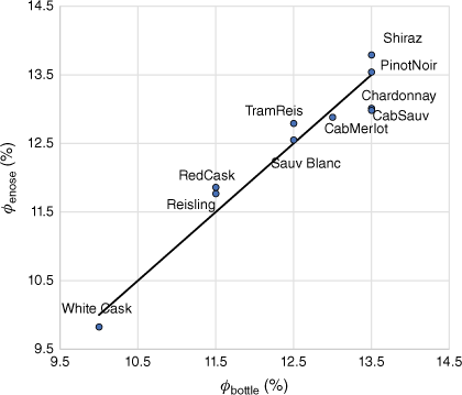
As an example of the use of principal-component analysis to extract features from a dataset, an eight-sensor electronic nose ‘sniffed’ a number of commercial Australian wines. A principal-component analysis on the autoscaled data showed 79% of the variance of the data could be expressed by four principal components. As ethanol is the predominant organic volatile constituent, it is not surprising that a principal-component regression against the ethanol volume fraction gave a reasonable fit (see Fig. 1).
Principal-component regression (PCR) using four principal components of ethanol volume fraction in Australian wines from autoscaled electronic nose data from eight sensors. ϕbottle is the alcohol content indicated on the wine bottle and ϕenose is the calculated value from the PCR. Solid line is equality (unpublished data of author) (Cab, Cabernet; Sauv, Sauvignon; Sauv Blanc, Sauvignon blanc; TramReis, Traminer Reisling).
In the case of a continuously monitored odour source, the background-corrected or transformed signal from each sensor is measured with time and a mean and standard deviation taken from data that suitably represent the particular odour. If a particular odour can fluctuate over a wide range, it may be convenient to create two target outcomes of a ‘very smelly’ and ‘not so smelly’ versions of that odour. Methods that classify particular odours do not perform well with mixtures and the best results come from clear-cut situations.
Analysis of electronic-nose output
Bayes’ theorem
Here, we describe a Bayesian approach to obtain probabilities of membership of pre-defined odour classes, which thus falls into the domain of ‘supervised learning’.25 The sensor data, either raw voltages or transformed in some way, are considered normally distributed random variables. By taking sufficient data for training, there is benefit from the Central Limit Theorem, and actual distributions are often sufficiently normal for the purposes of assigning test odours. (This assumption is discussed further below.) The term ‘Bayesian analysis’ covers all uses of Bayes’ theorem (which is stated later). A subordinate theory, ‘Naïve Bayes analysis’ has been used widely for supervised learning, and was patented by the author for electronic nose data in 2007.26 Naïve Bayes has been used for gas sensing of air leaks in boreholes in coal mines,27 determining the presence of gasoline in fire debris28 and determining the source of environmental oil spills.29 The qualifier ‘naïve’ indicates that the options are completely independent, with no correlation between the probabilities. This is a convenient assumption that simplifies calculations, but may not hold for electronic nose data. The results of using the Naïve Bayes approach against a more formal analysis of a multivariate normal distribution are investigated in the analysis of the breath of diabetes patients below.
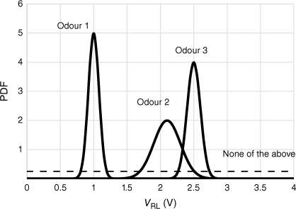
The principle of the method is illustrated in Fig. 2. A single sensor that has different responses to three odours is shown. A sensor voltage near 1 V clearly is ascribed to Odour 1. Between 2 and 2.5 V, there is a transition from Odour 2 to Odour 3. The dashed line represents a low likelihood of an odour that the electronic nose has not been trained to detect, and where its probability density function (PDF) is greater than those of Odours 1, 2 and 3, it becomes the most probable result.
Representation of probability density functions (PDFs) of a single electronic nose sensor to three odours. Dashed line is a constant, small rectangular PDF, with area 1, assigned to ‘none of the above’.
Bayes’ theorem states that the probability of an hypothesis given some evidence P(H|E)A is the product of the probability of the evidence given the truth of the hypothesis P(E|H) multiplied by the prior probability of the hypothesis P(H) and normalised by the probability of the evidence P(E). The probability of the evidence given the truth of the hypothesis P(E|H) is also the likelihood of the hypothesis given the evidence , which is obtained from the PDF of the distribution. The proof of the form used in Eqn 1 is completed by observing that, by the law of total probability, the probability of the evidence P(E) is the sum of the conditional probabilities of all the hypotheses considered.
Therefore, for a number of discrete possible hypotheses H1…n, Bayes’ theorem for the ith hypothesis is:
The sum in the denominator of Eqn 1 is over all possible hypotheses (in the example, Odours 1, 2 or 3 and ‘none’). Writing Eqn 1 in terms of the output voltage of a sensor VRL and Odours 1 … 3 and ‘none’:
If we have trained the sensor for each of the odours by measuring sensor voltages when exposed to each odour in turn, and we know the form of the distribution of the measured voltages, then for any measured test voltage (VRL), we may calculate the likelihood (below) as the PDF at VRL:
For a normally distributed sensor output with mean voltage V̅ and standard deviation s, the likelihood is the PDF of
taken at VRL. For ‘none of the above’, the PDF is the reciprocal of the range of possible voltages. To calculate the probabilities of each outcome given the measured sensor voltage for the unknown odour, a prior probability must be assigned to each potential odour, that is, the probability of a particular odour before we have made any measurements. A so-called ‘flat prior’ simply assigns an equal prior to each possible outcome; here, for four outcomes, the prior would be 0.25. This is often used when there is no particular reason to expect one outcome over any others. However, for the example problem, even if we do not favour any of the target odours, it may be that we do expect an assigned outcome, with ‘none’ being least likely. In this case, for example, the choice might be P(Odour1) = P(Odour2) = P(Odour3) = 0.3 and P(none) = 0.1. Wang et al.17 cite knowing the correct hypothesis model for the priors as a problem but experience of the author shows that the choice of priors is not so important for electronic nose data unless there is a large mismatch between the target options.
The Naïve Bayes approach to dealing with multiple sensors is to assume that each sensor responds independently of the others. This is unlikely to be true, given that MOS sensors operate on the same principle and are likely to have a generic response to classes of chemicals (such as VOCs). How this assumption holds up for the examples in this paper will be discussed later. However, Naïve Bayes accommodates multiple sensors nicely, by taking each sensor in turn and applying Eqn 1, with the prior for sensor j + 1 being the result of the previous calculation for sensor j. Starting with the first sensor with output voltage V1 for the test atmosphere, we may calculate the probability for each odour (and ‘none’) given the known distributions from the training phase (Eqn 2 with voltage V1). For Odour i having prior probability P(Odouri):
As before, the sum in the denominator is over all odours. The second sensor with measured voltage V2 is then introduced:
P(Odouri)|(V1,V2) reads ‘the probability that the unknown odour is Odour i given the output of sensors 1 and 2’. Substituting P(Odouri)|(V1) from Eqn 3:
Note we now have the product of likelihoods multiplied by the original prior probability. Generalising for k sensors:
where the product is over the likelihoods of l = 1…k sensors for the given Odour i, and the sum in the denominator is over j = 1…n odours.
If the assumption of independence is not supported (that is, ignoring the statistical niceties, if the assumption causes us to make the wrong decision), the data from many (k) sensors (V) may be fitted to a multivariate normal distribution, taking into account the covariance between the sensor outputs.
V̅ is the vector of k means, and Σ the k × k covariance matrix. The probability of a particular odour is then calculated directly from Bayes’ theorem using the multivariate PDF. In contrast to the Naïve Bayes approach, all the information about the sensor responses is in the multivariate distribution:
The use of Bayes’ theorem only requires a knowledge of the distribution of each sensor output for each odour (or its multivariate equivalent), with the likelihood calculated from the PDF of the assigned distribution. Two examples are given that have very different kinds of data, and with resulting possible different distributions. The first is sensing odours in an abattoir, with three sites being the possible source of an odour. The data (not collected by the author) are a long time series of the sensor output for each source of odour. The dispersion of the output is attributed to drift of the intensity of the odour itself, and (to a lesser degree) drift of the sensors. Although the drift is unlikely to be normally distributed, the dispersion is not great, and a normal distribution appeared to treat the data adequately. For the second example, breath samples from patients with and without diabetes, the dispersion is entirely from the differences in patients and, again, a normal distribution suffices, although a log-normal distribution may be better. However, in each case, it is not so obvious that a normal distribution is the ‘correct’ distribution. We therefore explore the simplest distribution with the least assumptions, a rectangular distribution between the maximum and minimum sensor outputs. This is shown in Fig. 3 for the hypothetical example of Fig. 2.
Example of Fig. 2 assuming rectangular distributions plotted, for each odour, across V̅ ± 3 s.d. for each sensor.
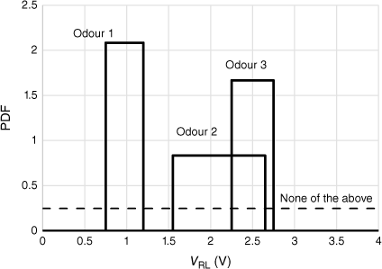
The likelihood is therefore a constant within the range chosen; for real data, this can be between the maximum and minimum of the recorded output or within plus or minus a number of standard deviations. Where the output is over an extended range, the PDF is smaller (the area ≡ 1) and so where there is competition, this odour will lose out to one with a more concentrated range (in Fig. 3, Odour 3 has a greater PDF than Odour 2 and will be preferred in the region of overlap). As before, outside the range of any of the sensors, ‘none of the above’ will prevail. The PDF to insert in Eqn 2 is then the result of the test
where Vmax(Odouri) and Vmin(Odouri) are the maximum and minimum voltage outputs for Odour i.
For ‘none’, as before:
Because the range of the output of the sensor will always be greater than any interval for a particular odour, and therefore the PDF less, ‘none’ will prevail only outside the ranges of odours.
Voting among multiple sensors
Another simplification is to determine P(Odouri|Vl) by Eqn 2 for each sensor independently and then award the assignment of odour to the one that has most ‘votes’, i.e. the odour for which most sensors record their maximum probabilities. This only is possible for three or more sensors, and for even numbers of sensors, some tie-break rule must be determined. However, combined with a rectangular distribution, this could be implemented with very little computing.
Examples
Two examples are given, both using data supplied by E-Nose Pty Ltd (c/o G. Bell, see https://e-nose.biz/). The E-nose instruments use up to six MOS sensors, together with, for some devices, temperature and humidity sensors.30,31 A description of each experiment is given, but the data are used ‘as is’ to provide examples of the different analysis approaches described above.
Data analysis was performed in Microsoft 365 Excel (ver. 2403 Build 16, Redmond, WA, USA) and MATLAB 2023a (The MathWorks Inc., Natick, MA, USA, see https://www.mathworks.com).
Data from a NSW abattoir
In 2006 and 2007, E-Nose Pty Ltd undertook a project for the New South Wales (NSW) Meat and Livestock Association, visiting several sites, setting up a five-sensor E-nose with sensitivity to a range of VOCs at each site. The illustrative data used here are from three sites at an abattoir: a lairage area, a rendering area and site called ‘Basement’. Data were collected over a 24-h period to provide the calibration. The method is tested by random segments of a few hours taken near each site some days later. Considerably more data were collected during the study, with the selection used here to demonstrate the approach to data analysis.
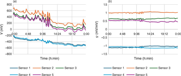
The output of each sensor was a voltage in the range −2 to +2 V. The sensor output rose and fell during the day, but the aim of the analysis is to assign the source of the odour, not its strength. Because the sensor outputs are highly correlated, the effect of the changing intensity of the odour can be reduced by dividing through by the value of one sensor. An effective alternative is to ‘row autoscale’, that is, to mean centre the data and divide by the sample standard deviation of the row elements. The result on the calibration data from Site 3 (‘Basement’) is shown in Fig. 4.
(a) Raw data from Site 3 (‘Basement’) over a 24-h period. (b) Row-autoscaled Site 3 data ψ = (V − V̅) ÷ s. V is the sensor output voltage, V̅ is the mean voltage and s the sample standard deviation of the five channels.
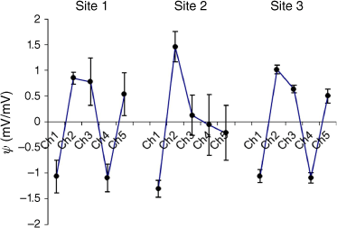
A comparison of transformed sensor output for the three sites is shown in Fig. 5. Error bars are ±2 standard deviations (s.d.) about the mean.
Mean row standardised sensor output (Ch1–Ch5) for each of three sites. Error bars are ±2 s.d.
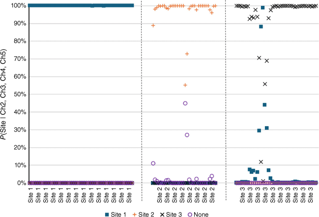
The Naïve Bayes model was then run on the three test sets. As standardisation causes the loss of a degree of freedom, the assignments used transformed data from sensors 2 to 5. There was 100% correct assignment for Sites 1 and 2, and 95% (41 of 43) correct assignment for Site 3 (Fig. 6). It is seen that the pattern of responses for Sites 1 and 3 are similar, and the erroneous Site 3 results do assign the odour to Site 1. The results from Site 2 showed the assignment ‘none’ showed significant probabilities on occasions during the run but they did not reach 50%.
Probabilities of site origin assigned to odours when sensors take data from each site in turn (x-axis label). Closed squares, odour assigned to Site 1; orange pluses, odour assigned to Site 2; black crosses, odour assigned to Site 3; open purple circles, none. Data taken at each site: Site 1: 5 days after calibration, duration 9 h, number of data points 54. Site 2: 2 days after calibration, duration 2:45 h, number of data points 34. Site 3: 2 days after calibration, duration 3:30 h, number of data points 43.
Breath-testing diabetes patients
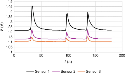
In 2000, in a collaboration between Diabetes Australia and E-Nose Pty Ltd, breath samples from 28 subjects were subjected to analysis by a three-sensor electronic nose. The sensors were MOS sensors from Figaro Ltd, with sensitivities to different classes of VOCs. Each person was asked to blow into a tube for a certain time and breath was monitored by the electronic nose. A typical response is shown in Fig. 7.
Sensor data used in this study were the maximum voltage from each sensor and the half-width at half maximum (HWHM) of each breath. Two to four breaths were collected from each person, giving a total of 94 sets of sensor readings. Whether or not the person was diagnosed with diabetes (Y or N) and their blood glucose level (mmol L–1) were also made available. A total of 14 subjects had been diagnosed with diabetes and 14 had not. In total, 12 runs were taken at random from the diabetic cohort and 13 from the non-diabetic, leaving 33 Y and 36 N to calibrate the model. The calibration data sets were tested for a normal distribution and two sets in each cohort were rejected, having Grubbs outliers (tested at >95% confidence) for one sensor.
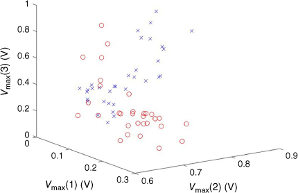
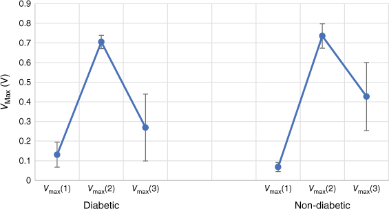
Different combinations of the sensor data were investigated, but here, we present only the maximum voltages from the three sensors without further transformation. A plot of the raw data is given in Fig. 8. It is seen that while there are areas of separation, there is also considerable overlap between diabetic and non-diabetic subjects. This is seen in the similarities of the mean VMax of each sensor to each condition (Fig. 9).
Peak maxima for three MOS sensors for diabetic (open red cicles) and non-diabetic (blue crosses) subjects.
Mean ± 2 s.d. for the maximum sensor response to the breath of known diabetic and non-diabetic patients.
Using means and standard deviations of the calibration data, the Naïve Bayes model of Eqn 6 was applied to the test data. In addition, the use of a multivariate normal distribution, the use of rectangular distributions and the voting approach discussed above were also applied. Results are brought together in Table 2. Out of the 14 diabetic patients used for testing, 8 had glucose levels greater than 7 mmol L–1. The success rate for these patients was recorded separately. One set of the Y test data gave 100% probability of ‘none’ and was removed from the set.
| Method | Correct Y (%) | Correct Y for high glucose (>7 mM) (%) | Correct N (%) | |
|---|---|---|---|---|
| Naïve Bayes | 64 | 75 | 83 | |
| Bayes with multivariate normal distribution | 82 | 88 | 92 | |
| Bayes with rectangular distribution | 42 | 56 | 92 | |
| Naïve Bayes with voting | 73 | 88 | 58 |
Given the high degree of correlation found with MOS sensors, it may not be surprising that a multivariate normal distribution gives the best success rate. It is not clear why the simple vote among the sensors does so well for the correct Y, whereas this is reversed for the other methods, which give correct N more times than Y. The small sample size could well be responsible for these behaviours.
Discussion and conclusions
Postives and negatives of the Bayesian approach for identification of odours
Bayes’ theorem is a powerful tool for supervised learning of a multisensory electronic nose. If the assumptions about the distribution of data are correct, the provision of a probability of an outcome for each sensor is useful information not available to many ‘black box’ chemometric techniques. The method accepts any numerical data, and so other chemometric methods can be applied before Bayes’ theorem. It has been noted that Naïve Bayes suffers if there is just a single wrong input.32 Because probabilities are multiplied (Eqn 6), one value near zero ruins it for the rest. Perhaps this is why the voting approach did better than Naïve Bayes for the Y cohort of diabetics. A near-zero probability only counts as one vote against and allows other sensors to overrule it.
Less useful is that these Bayesian methods only work for the odours they have been calibrated for. Thus, a 50:50 mixture of two target odours will not necessarily be picked. (An extra category of ‘mixture’ can be created but this is not practical for all combinations). However, the diabetic example could be improved by treating high blood glucose positive subjects separately from other diabetics.
Alternatives for treating electronic nose data
The first question that must be answered is whether the purpose of the analysis is identification of an odour from a known list of potential targets. If the investigation is of an unknown mixture with a view to discover how many odours there might be, and how they group, then Bayes cannot be used and a non-supervised learning method, as discussed in the Introduction, will be employed. If the strength of the odour is to be quantified, again, Bayes will not help.
It appears that the modern artificial intelligence (AI) methods based on artificial neural networks (ANN) are becoming very powerful. Wang et al., in their comprehensive review of 2023,17 highlight Extreme Learning Machine (ELM),33 which is described as a ‘new fast-learning algorithm, which randomly initialises the input weight, and analyses it to determine the output weight of the network’. Further improvements have been reported to cope with abnormal unknown odours34 and simultaneous identification and concentration of the target gas.35 Advances in the design of the electronics of portable electronic noses have led to the use of ‘edge computing’ in which data are directly processed on a microprogrammed control unit.36 This reduces the dependence on external devices, such as computers in the cloud, while allowing very sophisticated ANN models to be run on each sensor before coming together in a ‘sensor swarm’.
As with all analytical devices, if the original data are sufficiently clear, clever data processing will not be needed. However, electronic nose output is rarely clear-cut, and has benefitted from the sophistication of modern methods of analysis, like the Bayesian approaches discussed here.
Ethics
The study on diabetes received appropriate approval from The Royal North Shore Hospital in 2000.
Supplementary material
The data and calculations for the two examples are contained in Files S1 (Diabetes) and S2 (meat works). Supplementary material is available online.
Data availability
All the data used in the statistical analysis in this paper are available as Supplementary material.
Acknowledgements
The author thanks Dr Graham Bell of E-Nose Pty Ltd for making data available, and for critically reading a draft of the manuscript. He also acknowledges discussions with Professor Thomas Walczyk concerning the rectangular distribution as a defensible alternative to a Gaussian distribution. D. Brynn Hibbert was the recipient of the 2023 Leighton Memorial Medal.
References
1 del Valle M. Sensors as green tools in analytical chemistry. Curr Opin Green Sustain Chem 2021; 31: 100501.
| Crossref | Google Scholar |
3 Wang M, Chen Y. Electronic nose and its application in the food industry: a review. Eur Food Res Technol 2024; 250: 21-76.
| Crossref | Google Scholar |
4 Vinicius da Silva Ferreira M, Barbosa JL, Jr, Kamruzzaman M, Barbin DF. Low-cost electronic-nose (LC-e-nose) systems for the evaluation of plantation and fruit crops: recent advances and future trends. Anal Methods 2023; 15: 6120-6138.
| Crossref | Google Scholar | PubMed |
5 John AT, Murugappan K, Nisbet DR, Tricoli A. An outlook of recent advances in chemiresistive sensor-based electronic nose systems for food quality and environmental monitoring. Sensors 2021; 21: 2271.
| Crossref | Google Scholar | PubMed |
6 Giannoukos S, Brkić B, Taylor S, Marshall A, Verbeck GF. Chemical sniffing instrumentation for security applications. Chem Rev 2016; 116: 8146-8172.
| Crossref | Google Scholar | PubMed |
7 Lee S, Kim M, Ahn BJ, Jang Y. Odorant-responsive biological receptors and electronic noses for volatile organic compounds with aldehyde for human health and diseases: a perspective review. J Hazard Mater 2023; 455: 131555.
| Crossref | Google Scholar | PubMed |
8 Wilson AD, Forse LB. Potential for early non-invasive COVID-19 detection using electronic-nose technologies and disease-specific VOC metabolic biomarkers. Sensors 2023; 23: 2887.
| Crossref | Google Scholar | PubMed |
9 Kabir KMM, Baker MJ, Donald WA. Micro- and nanoscale sensing of volatile organic compounds for early-stage cancer diagnosis. Trends Analyt Chem 2022; 153: 116655.
| Crossref | Google Scholar |
10 Ollé EP, Farré-Lladós J, Casals-Terré J. Advancements in microfabricated gas sensors and microanalytical tools for the sensitive and selective detection of odors. Sensors 2020; 20: 5478.
| Crossref | Google Scholar | PubMed |
11 Khorramifar A, Karami H, Lvova L, Kolouri A, Łazuka E, Piłat-Rożek M, et al. Environmental engineering applications of electronic nose systems based on MOX gas sensors. Sensors 2023; 23: 5716.
| Crossref | Google Scholar | PubMed |
12 Figaro Engineering Inc. Gas Sensors & Modules. Japan: Figaro Engineering Inc; 2018. Available at https://www.figaro.co.jp/en/product/sensor/ [Verified 21 April 2024].
14 Yan J, Guo X, Duan S, Jia P, Wang L, Peng C, et al. Electronic nose feature extraction methods: a review. Sensors 2015; 15: 27804-27831.
| Crossref | Google Scholar | PubMed |
15 Hibbert DB. Vocabulary of concepts and terms in chemometrics (IUPAC Recommendations 2016). Pure Appl Chem 2016; 88: 407-443.
| Crossref | Google Scholar |
16 Luo J, Zhu Z, Lv W, Wu J, Yang J, Zeng M, et al. E-Nose system based on fourier series for gases identification and concentration estimation from food spoilage. IEEE Sens J 2023; 23: 3342-3351.
| Crossref | Google Scholar |
17 Wang X, Zhou Y, Zhao Z, Feng X, Wang Z, Jiao M. Advanced algorithms for low dimensional metal oxides-based electronic nose application: a review. Crystals 2023; 13: 615.
| Crossref | Google Scholar |
18 Ge H, Liu J. Identification of gas mixtures by a distributed support vector machine network and wavelet decomposition from temperature modulated semiconductor gas sensor. Sens Actuators – B. Chem 2006; 117: 408-414.
| Crossref | Google Scholar |
19 González Martı́n Y, Cerrato Oliveros MC, Pérez Pavón JL, Garcı́a Pinto C, Moreno Cordero B. Electronic nose based on metal oxide semiconductor sensors and pattern recognition techniques: characterisation of vegetable oils. Anal Chim Acta 2001; 449: 69-80.
| Crossref | Google Scholar |
20 Cho JH, Kurup PU. Decision tree approach for classification and dimensionality reduction of electronic nose data. Sens Actuators – B. Chem 2011; 160: 542-548.
| Crossref | Google Scholar |
21 Gardner JW, Boilot P, Hines EL. Enhancing electronic nose performance by sensor selection using a new integer-based genetic algorithm approach. Sens Actuators – B. Chem 2005; 106: 114-121.
| Crossref | Google Scholar |
22 Aznan A, Gonzalez Viejo C, Pang A, Fuentes S. Rapid detection of fraudulent rice using low-cost digital sensing devices and machine learning. Sensors 2022; 22: 8655.
| Crossref | Google Scholar | PubMed |
23 LeCun Y, Bengio Y, Hinton G. Deep learning. Nature 2015; 521: 436-44.
| Crossref | Google Scholar | PubMed |
24 Wang Z, Yu Y, Liu J, Zhang Q, Guo X, Yang Y, et al. Peanut origin traceability: a hybrid neural network combining an electronic nose system and a hyperspectral system. Food Chem 2024; 447: 138915.
| Crossref | Google Scholar | PubMed |
27 Pan H-y, He S-n, Zhang T-j, Song S, Wang K. Application of an improved naive Bayesian analysis for the identification of air leaks in boreholes in coal mines. Sci Rep 2022; 12: 16081.
| Crossref | Google Scholar | PubMed |
28 Bogdal C, Schellenberg R, Höpli O, Bovens M, Lory M. Recognition of gasoline in fire debris using machine learning: part I, application of random forest, gradient boosting, support vector machine, and naïve Bayes. Forensic Sci Int 2022; 331: 111146.
| Crossref | Google Scholar | PubMed |
29 Li J, Hibbert DB, Fuller S, Cattle J, Pang Way C. Comparison of spectra using a Bayesian approach. An argument using oil spills as an example. Anal Chem 2005; 77: 639-644.
| Crossref | Google Scholar | PubMed |
32 Zhao Y, Tian S. Identification of hidden disaster causing factors in coal mine based on Naive Bayes algorithm. J Intell Fuzzy Syst 2021; 41: 2823-2831.
| Crossref | Google Scholar |
33 Jian Y, Huang D, Yan J, Lu K, Huang Y, Wen T, et al. A novel extreme learning machine classification model for e-Nose application based on the multiple kernel approach. Sensors 2017; 17: 1434.
| Crossref | Google Scholar | PubMed |
34 Zhang L, Deng P. Abnormal odor detection in electronic nose via self-expression inspired extreme learning machine. IEEE Trans Syst Man Cybern Syst 2019; 49: 1922-1932.
| Crossref | Google Scholar |
35 Wang T, Zhang H, Wu Y, Chen X, Chen X, Zeng M, et al. Classification and concentration prediction of VOCs with high accuracy based on an electronic nose using an ELM-ELM integrated algorithm. IEEE Sens J 2022; 22: 14458-14469.
| Crossref | Google Scholar |
36 Wang T, Wu Y, Zhang Y, Lv W, Chen X, Zeng M, Yang J, Su Y, Hu N, Yang Z. Portable electronic nose system with elastic architecture and fault tolerance based on edge computing, ensemble learning, and sensor swarm. Sens Actuators – B. Chem 2023; 375: 132925.
| Crossref | Google Scholar |


