

Defining humpback whale (Megaptera novaeangliae) potential distribution in the Great Barrier Reef Marine Park: a two-way approach
Consuelo M. Fariello A B * , Jan-Olaf Meynecke A B C * and Jasper de Bie A B C *
A
B
C
Abstract
Humpback whale (Megaptera novaeangliae) populations have been recovering from whaling but are now facing threats from changing food availability due to ocean warming and changes in habitat suitability. There is uncertainty over whether opportunistic observations can produce reliable species distribution models (SDMs) and adequately inform conservation management.
To compare SDMs for humpback whales in the Great Barrier Reef Marine Park based on different opportunistic sightings datasets and evaluate the impact different sources of opportunistic data have on our understanding of humpback whale habitat relationships.
Maximum entropy modelling (Maxent) was used to create predictive models for humpback whale distributions. Sighting data from citizen science and opportunistic observations from various other databases were used. Models were compared to evaluate disparities and predictive capabilities.
Distinct environmental variables [bathymetry, distance to the coast] were identified as the most relevant for each SDM. The best-fitting model diverged from an existing model, with humpback whale distribution predicted to be closer to shore. Areas with the highest habitat suitability were concentrated in the north-eastern coastal region across all models developed in this study.
This study demonstrates that, with careful application and consideration, citizen science data can enhance our understanding of humpback whale distributions and contribute to their conservation. The research underlines the importance of embracing diverse data sources in SDM, despite the challenges posed by opportunistic data.
The study provides valuable insights for conservation management and informs strategies to protect humpback whale populations in changing environmental conditions.
Keywords: citizen science, climate change, GBRMP, humpback whale, Maxent, Megaptera novaeangliae, opportunistic data, SDM, species distribution model.
Introduction
Baleen whales are considered globally important for their ecosystem services, their economic and intrinsic values (Clapham 2001; O’Connor et al. 2009), their influence on oceanic dynamics through top-down (predation) and bottom-up (nutrient fertilisation) processes (Roman et al. 2014; Ratnarajah et al. 2016), and for their potential as indicators of ocean health (Fleming et al. 2016). Humpback whales (Megaptera novaeangliae; hereafter HWs) are a widespread species of baleen whale that performs one of the longest migrations of all baleen whale species, migrating from polar feeding grounds to tropical waters for mating and calving (Dawbin 1966; Chaloupka and Osmond 1999; Rasmussen et al. 2007).
On the breeding grounds, HWs’ distribution and behaviour are influenced by sea surface temperature (SST), distance to the coast, bathymetry, and distance to the reef (Ersts and Rosenbaum 2003; Johnston et al. 2007; Rasmussen et al. 2007; Oviedo and Solís 2008; Smith et al. 2012; Meynecke et al. 2020). HWs breed close to shore, in shallow and warm waters (21.1–28.4°C; Rasmussen et al. 2007), likely to benefit the growth and development of calves (Whitehead and Moore 1982; Craig and Herman 1997; Ersts and Rosenbaum 2003; Oviedo and Solís 2008; Rosenbaum et al. 2014). They prefer breeding habitats at depths of 20–50 m (May-Collado et al. 2005; Guidino et al. 2014; Derville et al. 2019; Smith et al. 2021) and are consistently located near (<10 km) reefs, islands or continents (Ersts and Rosenbaum 2003; Lindsay et al. 2016). Although chlorophyll a and salinity may not be major drivers in breeding areas, they could still play a role in the habitat preferences of HWs. The substantial river runoff in the Great Barrier Reef Marine Park (GBRMP) is known to cause local variations in salinity and concentrations of chlorophyll a, particularly during the rainy seasons (Brodie et al. 2012; Devlin et al. 2012, 2015).
Species distribution models (SDMs) are valuable tools for studying HWs due to their migratory nature, which makes investigating their distribution patterns and behaviour challenging. SDMs, such as maximum entropy modelling (Maxent), use environmental factors and species occurrence data to estimate suitable habitats beyond the sampled areas. Maxent has been widely applied in cetacean research (Smith et al. 2012; Bombosch et al. 2014; Pacheco et al. 2021). For example, in research from Bombosch et al. (2014), Maxent models of HWs and Antarctic minke whales were used as a planning tool for seismic surveys to reduce the impact of anthropogenic noise on marine mammals in the Southern Ocean. Their findings demonstrated the efficacy of using Maxent models to inform survey planning and minimise potential disturbances to these cetacean species in the region. Pacheco et al. (2021) constructed Maxent models to predict potential habitats for breeding HWs in the Southeast Tropical Pacific. By identifying distinct potential habitats for breeding HW groups, including those with calves, their research suggests specific management actions such as limiting whale-watching boats in the presence of mother–calf pairs and restricting gillnet use to mitigate entanglements, which can enhance the recovery and protection of these whale populations. In Australia, Smith et al. (2012) used this approach to determine two important breeding areas for HWs in the GBRMP. Their findings also revealed a significant overlap between the main breeding ground of HWs and the inner shipping route, providing valuable insights for conservation management and spatial planning.
Maxent uses occurrence data of the species and environmental variables layers as input to predict suitable habitats for a given species based on the environmental characteristics of the known occurrences. Maxent can incorporate presence-only data into the analysis (i.e. using bias files), unlike other modelling methods, particularly when this type of data is available (Phillips et al. 2006). Its output is then an index of environmental suitability for the species, where higher values indicate a prediction of better conditions.
Maxent ideally relies on random or representative sampling throughout the landscape. However, the full details of opportunistic sampling efforts are often unknown, a common scenario in ecological studies. Despite this, opportunistic data, even with its limitations, can offer valuable insights into species distributions when analysed with an understanding of their inherent biases and limitations. Sampling bias is typically described as the uneven representation of species distributions resulting from data collection biased towards well-surveyed or easily accessible areas (Hijmans et al. 2000; Reddy and Dávalos 2003; Kadmon et al. 2004). This clustering of records, possibly related to opportunistic observations, can result in a biased habitat suitability prediction through overfitting of spatially autocorrelated data (Radosavljevic and Anderson 2014). Furthermore, higher levels of importance may be assigned by Maxent to environmental variables that are typical for a region of intensive sampling (Ward 2006). These factors can significantly impact model outcomes, potentially resulting in the overrepresentation of species populations, thereby affecting conservation efforts for the species under consideration (Reddy and Dávalos 2003). Addressing sampling bias can be achieved through bias-correcting techniques, including spatial rarefying and background selection using a bias file (Kramer-Schadt et al. 2013; Fourcade et al. 2014; Moua et al. 2020). Spatial rarefying involves subsampling the occurrence records to create a more even distribution across the study area, reducing the influence of localised sampling efforts (Phillips et al. 2017). Background selection using a bias file involves incorporating information about spatial biases in occurrence data to guide the selection of representative background locations (Kramer-Schadt et al. 2013). These techniques were tested in a study by Kramer-Schadt et al. (2013) to mitigate uneven sampling effort in the case of the Malay civet in Borneo, resulting in a significant improvement in the accuracy of model predictions. In addition to these techniques, species-specific tuning can enhance Maxent models’ quality and transferability (Elith et al. 2011). Species-specific tuning refers to adjusting model parameters or settings specifically for the target species being modelled, considering its ecological characteristics and requirements (Elith et al. 2011). Therefore, three potential options exist for improving Maxent model performance, including the two bias-correction approaches and species-specific tuning.
The availability of opportunistic species observations collected by scientists or citizen science groups is increasing (Dickinson et al. 2010; Gledhill et al. 2014). Citizen science data have proven useful for data-poor species and or in understudied regions (Bouchet et al. 2021; McCulloch et al. 2021; Noviello et al. 2021). However, there is uncertainty about how useful these observations are in quantitative analyses of species distributions (e.g. species distribution models [SDMs]) and if they are valuable in determining species–habitat relationships and distribution maps that can be applied to conservation and management. In the GBRMP, citizen science data has been collected for 27 years from whale-watching vessels (Atlas of Living Australia 2022; Australian Marine Mammal Centre 2022; Eye on the Reef 2022; Ocean Biodiversity Information System 2022), but no SDM has been produced using these data. Smith et al. (2012) used presence-only data collected from 2003 to 2007 along transect lines in the Border Protection Command (BPC) aerial surveillance program to identify two breeding areas for the population of HWs in the GBRMP and a region predominantly used during migration. Their findings revealed a significant overlap between the main breeding ground of HWs and a heavily used shipping route, providing valuable insights for conservation management and spatial planning. The addition of longer-term and broader data collected by citizen scientists may be useful to further understand the boundaries of breeding areas for HWs in the GBRMP.
Here, we compare distribution models for HW subpopulation E1 (Mackintosh 1942; Gambell 1976) in the GBRMP using opportunistic sightings with a previously developed SDM for the region (Smith et al. (2012). We assess the performance of a widely applied SDM technique, maximum entropy modelling (Maxent), to utilise different types of data and draw conclusions on future use.
Methods
Study site
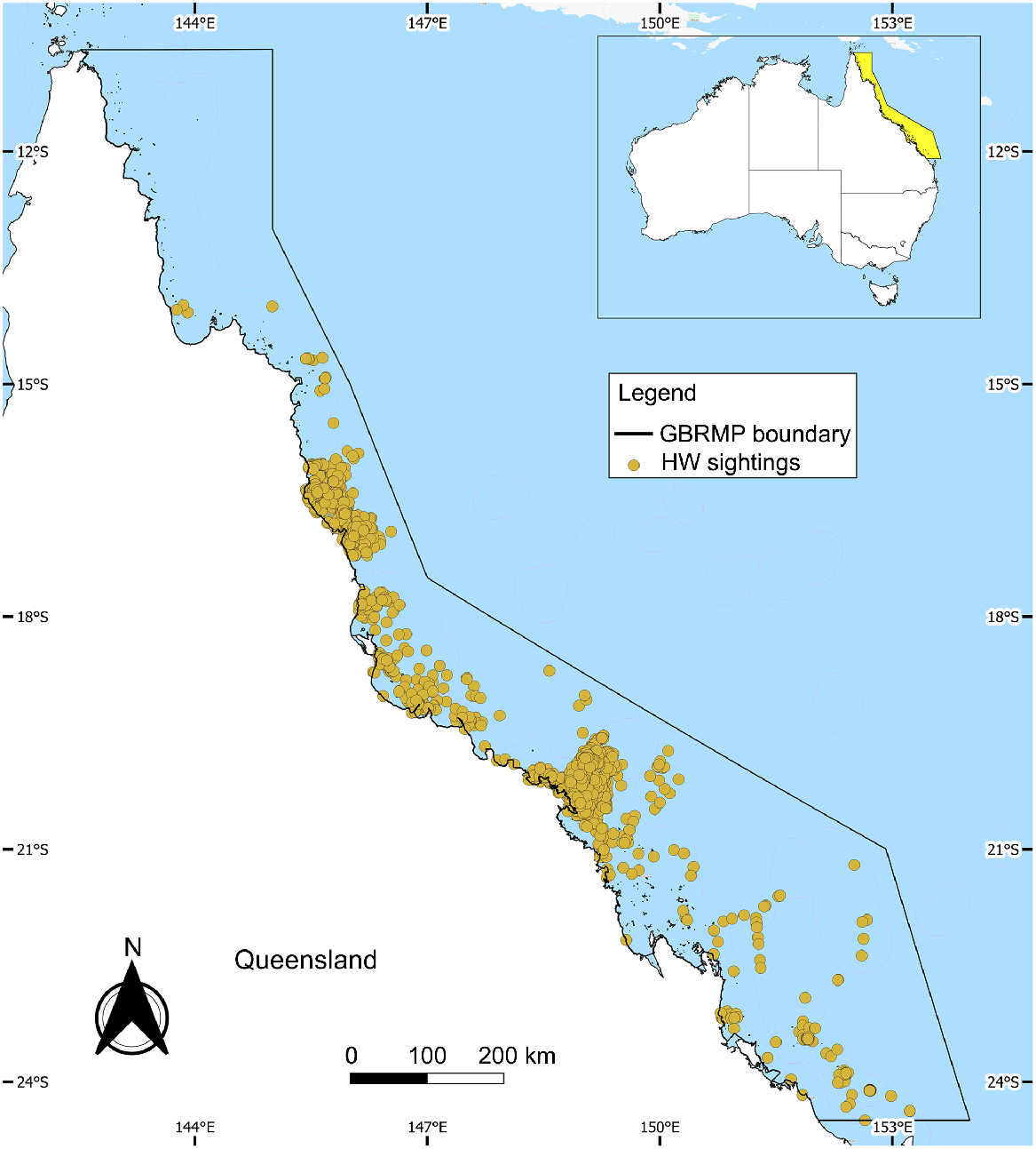
The GBRMP is located on the east coast of Australia (Fig. 1) and contains one of the world’s richest and most complex ecosystems. It has an average depth of 35 m in its coastal waters, whereas on outer reefs, continental slopes extend to depths of more than 2000 m (Great Barrier Reef Marine Park Authority 2019). The GBRMP has a tropical climate, with average temperatures in summer between 24°C and 33°C and in winter between 14°C and 26°C. The region has two distinct seasons, a dry, warm season and a hot, wet season. The Great Barrier Reef covers approximately 388,000 km2, with 99% of the area designated as GBRMP (Great Barrier Reef Marine Park Authority 2019). From June through November, the region is an important HW breeding area (Simmons and Marsh 1986; Smith et al. 2012).
Whale records
HW sightings were retrieved from Eye on the Reef (EOR), Atlas of Living Australia (ALA), Ocean Biodiversity Information System (OBIS), and the National Marine Mammal Database (NMMD). The largest number of records obtained for the study were from EOR, consisting of 3640 observations collected between 2000 and 2020. EOR is a monitoring and assessment program in the GBRMP, where staff from tourist dive boats collected standardised biological information regarding the reef’s health at frequently visited sites. This includes recording opportunistic HW sightings during each trip. ALA, OBIS and NMMD are open-access collaborative databases on biodiversity. These databases employ a combination of methods to collect data from various sources, including citizen science programs, ship-based and aerial surveys, partnerships with organisations, and data digitisation. The associated data from these (88, 189, and 19 sightings, respectively) are presence-only opportunistic records collected non-systematically from 2000 to 2020. Although only limited information is available regarding their research efforts on HWs, collected data have undergone quality checks to ensure accuracy and reliability. Quality checks include location, time and date validation, data cleaning and filtering, cross-checking with other databases, and expert review to ensure data accuracy.
The datasets utilised in this study, in contrast to the approach by Smith et al. (2012), extend beyond the peak breeding months of July and August. This broader temporal scope aligns with research indicating potential changes in the timing of both migration and breeding activities (Franklin et al. 2011; Ramp et al. 2015; Meynecke et al. 2017; Torre-Williams et al. 2019; Gosby et al. 2022).
Environmental variables
Salinity, SST and chlorophyll a values were obtained from BioOracle (Tyberghein et al. 2012). The long-term averages for these data span a time period of 2000–2014 at a spatial resolution of approximately 8.3 km. Bathymetry was obtained from eAtlas (Beaman 2020) at a raster resolution of 100 m. Pixels with positive bathymetry values, corresponding to islands between the GBRMP and part of the coastline, were removed from the raster.
Distance to the coast and distance to the reef were derived using ArcGIS Pro ver. 2.9.0 software geoprocessing tools. For distance to the coast, each pixel in the raster represents the distance in metres from the centre of that pixel to the coastline of the GBRMP (excluding any islands). Geoprocessing tools were utilised to calculate the distance of each point within the study domain to the coast and convert these distance values into a raster format. Similarly, distance to the nearest reef was computed using the same process, measuring the distance from each point to the closest reef rather than the GBRMP coast.
In this study, ‘Coastal Waters’ or ‘inshore’ areas adhere to the definition provided by Geoscience Australia (2023), based on the United Nations Convention on the Law of the Sea (UNCLOS). This approach provides a consistent framework for comparison between datasets. Under this definition, ‘Coastal Waters’ areas extend from the territorial sea baseline up to a line 3 nautical miles seaward.
All grids were resampled to a consistent 0.085° (~8.5 km) grid resolution and reprojected to the standard WGS84, EPSG 4326 geographic projection in ArcMap, ensuring uniform geographic bounds and cell size for all variables.
Bias correction
Two different bias-correcting methods were applied to account for spatial clustering of HW sightings data (Fig. 1). First, data were spatially rarefied at 10-km resolution using the ‘spThin’ R package (Aiello-Lammens et al. 2015; Duengen et al. 2022). This resulted in a total of 2584 (92.9%) records being removed from the 2000–2014 dataset, leaving 197 records (Model C; Table 1). Second, we employed the ArcGIS ‘Sample by buffered MCP’ tool for background selection. This approach involved selecting background points within a maximum radial distance of 5 km from known occurrences, with a cap of 10,000 points. This method aligns with established practices in the field (Phillips et al. 2009; Barbet-Massin et al. 2012; Brown 2014).
| Model ID | Occurrence data span | N° of sightings used | Background selection via bias file | Spatial rarefying | Maxent parameters | ||
|---|---|---|---|---|---|---|---|
| RM | Features | ||||||
| A | 2000–2014 | 2781 | 1 | Auto features | |||
| B | 2000–2020 | 3936 | 1 | Auto features | |||
| C | 2000–2014 | 197 | (x) | 1 | Auto features | ||
| D | 2000–2020 | 254 | (x) | 1 | Auto features | ||
| E | 2000–2014 | 2781 | (x) | 1 | Auto features | ||
| F | 2000–2020 | 3936 | (x) | 1 | Auto features | ||
| G | 2000–2014 | 197 | (x) | (x) | 1 | Auto features | |
| H | 2000–2020 | 254 | (x) | (x) | 1 | Auto features | |
| I | 2000–2014 | 197 | (x) | 0.5 | LQH | ||
| J | 2000–2020 | 254 | (x) | 1.5 | LQH | ||
| X | 2003–2007 | 90 | 1 | Auto features | |||
Table shows the data time span, the type of correction bias (if any) applied, the number of sightings and the Maxent parameters selected. (x) denotes the bias-correction method applied.
RM, regularisation multiplier, with L, Linear; Q, Quadratic, H, Hinge.
Maxent tuning
Maxent’s default parameters were used for Models A–H (Table 1). Subsequently, the best-fit models from each time span were optimised through tuning to enhance model performance. The best-fit Maxent models were selected based on the Bayesian Information Criterion (BIC) calculated with ENMTools (Warren et al. 2010). BIC was chosen for model selection because it penalises model complexity more strongly than other criteria (Burnham and Anderson 2002; Neath and Cavanaugh 2012; Kumar et al. 2015). The ENMeval package in R (Muscarella et al. 2014) was used to conduct the tuning process. For the best-fit models from each time span, 24 combinations were evaluated: six feature classes (L/LQ/H/LQH/LQHP/LQHPT; where ‘L’ linear, ‘Q’ quadratic, ‘H’ hinge, ‘P’ product transformation and ‘T’ threshold), and four Regularisation Multiplier (RM) values (from 0.5 to 3.5, with one unit increment). Using the two combinations that achieved the highest Akaike’s information criterion (AIC), the tuning process resulted in creating two Maxent models, Models I and J.
Model evaluation
Response curves were used to show how each variable affects the Maxent models’ overall predictions. They demonstrate how prediction probabilities of presence vary as each environmental variable is modified, using only one variable at a time. The jackknife test was used to assess the contribution of each variable in the models, providing insights into their explanatory power and unique information for the species’ potential distribution.
Maxent models were assessed using threshold-independent and threshold-dependent metrics to evaluate their performance. The area under the curve (AUC) of the receiver operating characteristic (ROC) curve served as a threshold-independent measure, quantifying the model’s discriminatory power. AUC values range from 0 to 1, where 0.5 signifies random prediction, and 1 indicates perfect discrimination between suitable and non-suitable habitats. Two metrics were employed for threshold-dependent evaluation: omission rate (OR) at the minimum training presence threshold and OR at the 10% training presence threshold. The expected value of the test OR at the minimum training presence threshold is 0, whereas at the 10% training presence threshold, it is 0.10. Higher-than-expected OR values indicate inadequate model performance (Boria et al. 2014). The Maxent algorithm calculates the OR in training and test data, representing the percentage of test locations predicted as unsuitable for the species (Phillips 2005).
To validate the representativeness of our dataset and comprehensive environmental coverage across the GBRMP compared to Smith et al. (2012), we conducted a niche overlap analysis (Lysy et al. 2014). The analysis was performed using the ‘nicheROVER’ R package. The variables for the analyses were distance to the shore, distance to the reef, SST, bathymetry, and salinity. The datasets used were the BPC sightings employed by Smith et al. (2012) compared to the dataset used for our best-performing model.
Model development
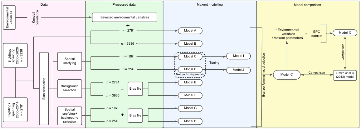
Data processing and statistical analysis were conducted using the following software versions: QGIS 3.22.5 (QGIS Development Team 2022), ArcGIS Pro 2.9.0 (Esri 2021), and R 4.2.0 (R Core Team 2022). Predictive models of HW distribution in the GBRMP were developed using the software Maxent 3.4.4 (Phillips et al. 2021). The first models (Models A and B) were developed using the full HW sightings dataset from 2000–2014 and 2000–2020 and used as the baseline models with no post-processing data (Table 1). Models C to J, our post-processed models, were developed to improve the performance of Models A and B, which would result in the creation of our best-fit model (Fig. 2). A comparison was made between two sets of models (Models A–B; C–D; E–F; G–H; I–J) to ensure the reliability of the 2000–2020 models despite the environmental predictors not aligning with the longer period of whale sightings. This approach was necessary due to the limited availability of environmental data in BioOracle, which only covered the years 2000–2014. The selection of the 2000–2014 period for the environmental data by BioOracle was based on the availability of satellite data used to generate the environmental models, ensuring the use of the most reliable and up-to-date information for that specific timeframe. Multi-collinearity among environmental variables was tested by calculating the Kendall correlation rank coefficient (Table 2). Correlated variables were identified using a threshold value of ±0.5 (Dormann et al. 2013). The variable that contributed the least information to the SDM according to the jackknife test was excluded for subsequent models’ development.
Methodological flow chart showing the sequential steps followed in this study: Maxent models were initially developed using 2000–2014 data, later expanded with 2015–2020 sightings. Model C, refined through bias corrections and tuning, was employed to reassess HW sighting data from Smith et al. (2012), validating Model C’s accuracy and facilitating a final comparison with Smith et al.’s model.
| Environmental variable | Salinity | SST | Bathymetry | Chlorophyll a | Distance to coast | Distance to reef | |
|---|---|---|---|---|---|---|---|
| Salinity | 1 | −0.862 | 0.261 | 0.609 | −0.126 | −0.027 | |
| SST | 1 | −0.209 | −0.570 | 0.054 | −0.002 | ||
| Bathymetry | 1 | 0.461 | −0.414 | −0.469 | |||
| Chlorophyll a | 1 | −0.396 | −0.135 | ||||
| Distance to coast | 1 | 0.239 | |||||
| Distance to the reef | 1 |
The best-fit model was compared with the model prediction of environmental suitability developed by Smith et al. (2012). Differences in response curves and variable contributions were analysed. Additionally, our model results showcased the most suitable areas for HWs within the GBRMP, highlighting these habitats through maps. This approach enabled the evaluation of habitat suitability congruence between the two models for HWs. To demonstrate the efficacy of our approach, Model X (Table 1) was developed by utilising an approximation of the BPC dataset (90 HW sightings collected between 2003 and 2007) and incorporating the environmental predictors and parameters from our best-fitting model. Locations of the HW sightings in the dataset used in Smith et al.’s (2012) research were estimated using georeferencing in QGIS before using them as input data in Maxent.
Results
Whale records
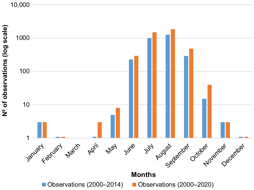
Observations followed the expected seasonal trend of HW presence in the GBRMP, with most observations (80%) occurring in July and August (Fig. 3). The monthly distribution of HW sightings post-filtering within the GBRMP (Supplementary Fig. S1) also depicts the peak of observations during July and August.
Model development
According to the Kendall correlation rank test, salinity, SST, and chlorophyll a were identified as correlated variables (Table 2). Based on the jackknife test, chlorophyll a contributed the least information to the full model and was excluded from subsequent models.
The niche overlap analysis revealed a significant 96% congruence (α = 0.99) between the environmental niches defined by our dataset and those identified in Smith et al. (2012).
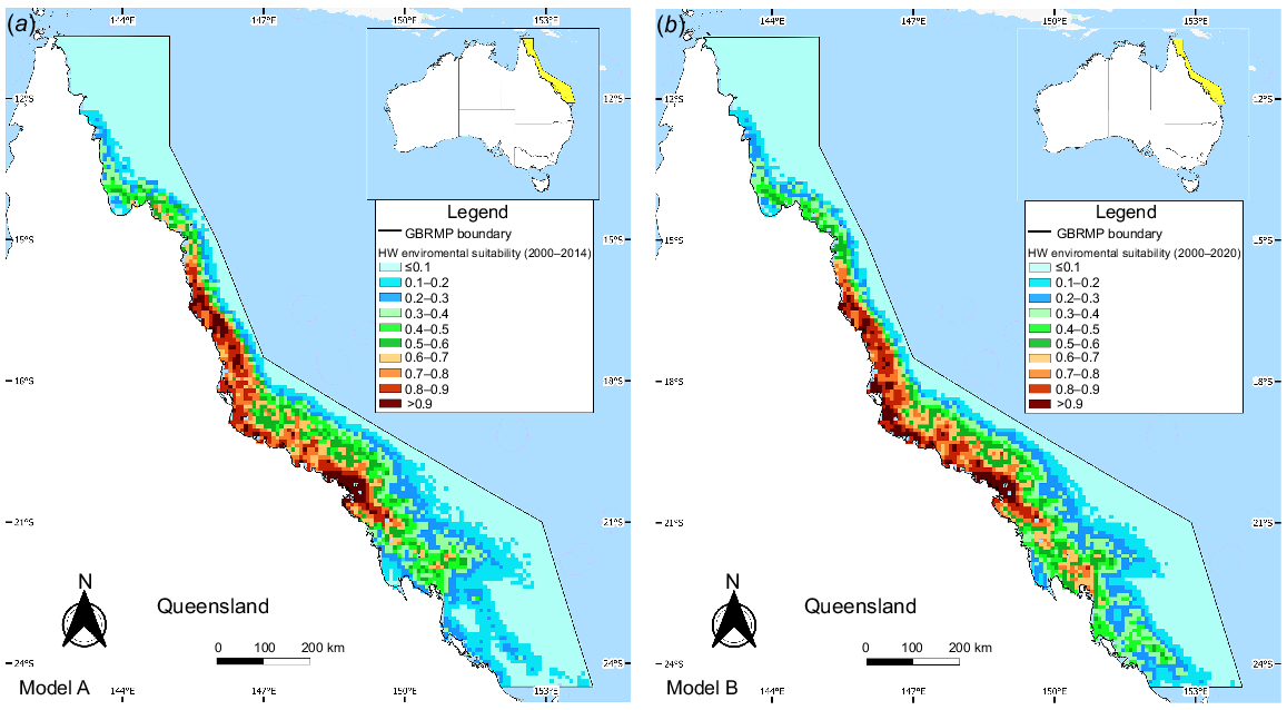
Both Models A and B suggested highly suitable areas (>0.7) were primarily concentrated near the coast, between 19°S and 21°S (Fig. 4). The average test AUC (Table 3) for both models exceeded 0.8, indicating the models are reliable at discriminating between suitable and non-suitable habitats. SST and distance to the coast contributed most to the overall performance of Models A and B, collectively explaining approximately 80% of the variation in species distribution (Table 4). The variables that contributed the least were bathymetry for Model A and distance to the reef for Model B. For both models, the variable with the most predictive power (highest AUC) when used in isolation was distance to the coast; therefore, it was the most significant driver for each model (Fig. S2). The variable with the least predictive power was distance to the reef for both models. The variable that decreases the AUC the most when omitted is SST for Model A and distance to the coast for Model B; therefore, they appear to have the most information not represented in the other variables. The response curves for both models A and B are similar (Fig. S3). Distance to the coast and SST values that correspond to high environmental suitability (>7) changed by no more than 0.5 units on average.
Environmental suitability for HWs in the GBRMP between (a) 2000–2014 (Model A) and (b) 2000–2020 (Model B). The colour scale denotes habitat suitability, ranging from 0 (light blue) to 1 (dark red).
| Model ID | AUC | OR (at 10 percentile training presence threshold) | OR (at minimum training presence threshold) | BIC score | Model rank | ||||
|---|---|---|---|---|---|---|---|---|---|
| Training data | Test data | Training data | Test data | Training data | Test data | ||||
| A | 0.856 | 0.843 | 0.097 | 0.131 | 0 | 0.007 | 39,085.5 | 7 | |
| B | 0.849 | 0.841 | 0.098 | 0.115 | 0 | 0.005 | 57,155.7 | 9 | |
| C | 0.833 | 0.813 | 0.097 | 0.13 | 0 | 0.017 | 3081.2 | 1 | |
| D | 0.83 | 0.817 | 0.099 | 0.118 | 0 | 0.008 | 4074.7 | 5 | |
| E | 0.804 | 0.784 | 0.097 | 0.124 | 0 | 0.004 | 40,049.7 | 8 | |
| F | 0.795 | 0.783 | 0.098 | 0.113 | 0 | 0.003 | 57,766.8 | 10 | |
| G | 0.772 | 0.739 | 0.098 | 0.142 | 0 | 0.006 | 3160.3 | 2 | |
| H | 0.772 | 0.749 | 0.099 | 0.122 | 0 | 0.008 | 4121 | 6 | |
| I | 0.845 | 0.811 | 0.097 | 0.157 | 0 | 0.022 | 3273.2 | 3 | |
| J | 0.826 | 0.816 | 0.099 | 0.11 | 0 | 0.008 | 3981.4 | 4 | |
Each model number corresponds to the models introduced in Table 1. The optimal model from all models (lowest BIC) is denoted by bold text, and the optimal models selected for tuning are in italics.
| Model ID | Relative variable contribution (%) | |||||
|---|---|---|---|---|---|---|
| Salinity | SST | Bathymetry | Distance to the coast | Distance to the reef | ||
| A | 6.2 | 39.1 | 3.5 | 43.9 | 7.3 | |
| B | 6.8 | 33 | 7.5 | 47.5 | 5.2 | |
In total, 10 Maxent models, with varying feature classes and RM, were evaluated for predicting HW distribution using different combinations of bias-correction methods. All models performed better than random, with training and test AUC values exceeding 0.7 (Table 3). Moreover, these models demonstrated low OR at the minimum predicted threshold, with values of 0 in the training data and below 0.02 in the test data. Additionally, at the 10th percentile training presence threshold, the models showcased OR values below 0.09 in the training data and below 0.16 in the test data. Model F had the highest BIC value and lowest rank. After bias correction, each method (spatial rarefying, implementation of a bias file, and both methods combined) resulted in a slightly lower testing AUC and a broader range of suitable habitats compared to models with no bias correction (Table 3). Evaluations of RM and feature class combinations for Maxent tuning are presented in Tables S1 and S2.
The analysis of relative contributions revealed that SST and distance to the coast emerged as the two key variables influencing the performance of Models C to J. These variables, on average, accounted for approximately 75% of the variation in species distribution across these models (Table 5). The jackknife plot of variable importance indicated that distance to the coast, when used alone, was the environmental predictor that had the greatest influence on Models C to J (Fig. S4). The variable that decreased the models’ AUC the most when excluded was also distance to the coast. On the other hand, distance to the reef had the lowest impact on models D, J, and I. In models C, E, G and H, the lowest impact was for salinity, and for Model F, it was SST.
| Model ID | Relative variable contribution (%) | ||||||
|---|---|---|---|---|---|---|---|
| Bias correcting method | Salinity | SST | Bathymetry | Distance to the coast | Distance to the reef | ||
| C | Spatial rarefying | 6.4 | 38.4 | 5.5 | 41.5 | 8.2 | |
| D | Spatial rarefying | 7.4 | 31.5 | 13.4 | 42.9 | 4.8 | |
| E | Bias file | 11.3 | 19.3 | 2.2 | 57.2 | 9.9 | |
| F | Bias file | 12.8 | 12.7 | 5 | 62.2 | 7.3 | |
| G | Both methods | 12.6 | 14.4 | 3.3 | 58.4 | 11.2 | |
| H | Both methods | 13.6 | 9.6 | 7.4 | 61.5 | 7.8 | |
| I | Tuning | 7 | 36.8 | 8.6 | 39.7 | 8 | |
| J | Tuning | 5.7 | 31.3 | 11.7 | 45.7 | 5.7 | |
Model results for the two different periods, 2000–2014 and 2000–2020, showed similar results (Fig. S5).
Comparison between the best-performing Maxent model and the existing model from Smith et al. (2012)
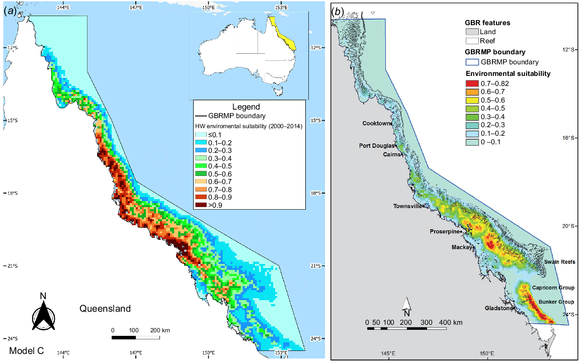
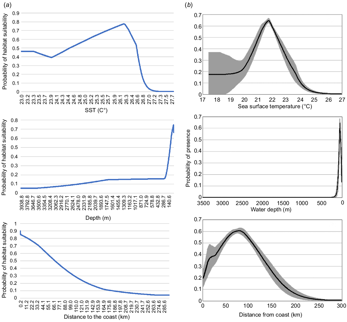
Model C emerged as the best-fit model (BIC value: 3081.2). It included the feature class LQH with an RM value of 0.5 (Table 1). Model C suggested the highest values of environmental suitability (0.7–0.99) between 15°S and 21°S (Fig. 5). In contrast, Smith et al. (2012) identified two core areas as highly suitable for HW based on their Maxent model. The first area is located approximately 100 km east of Proserpine, south of Mackay, and the second area is offshore of the Capricorn and Bunker groups of islands and reefs (Fig. 5). The response curves for Model C showed a preference of HW for waters between 7 and 33 m deep, with the highest probability at −11 m. In contrast, Smith et al.’s (2012) identified the highest values of environmental suitability (>0.7) at depths between 30 and 58 m, with the highest likelihood at −49 m (Fig. 6). Similarly, the marginal response curve for sea surface temperature (SST) differed between the models. Model C exhibited a range of 25.7–26.4°C with the highest value of 26.2°C, whereas Smith et al. (2012) reported a range of 21–23°C with the highest probability at 21.8°C. Additionally, Model C suggested HWs showed a preference for areas between 0.24 and 37 km from the coast, whereas Smith et al.’s (2012) identified a preference for areas between 60 and 110 km from the coast.
(a) Model prediction of average environmental suitability of the best-fitting model, Model C. (b) Model prediction of average environmental suitability between 2003 and 2007 developed in research by Smith et al. (2012). Colour scale denotes habitat suitability ranging from 0 (light blue) to 1 (dark red). GBR, Great Barrier Reef.
Response curves depicting the relationship between the predicted probability of HW occurrence and three environmental variables – SST, bathymetry, and distance to the coast. (a) Response curves for Model C developed in this study. (b) Response curves for Smith et al.’s (2012) model.
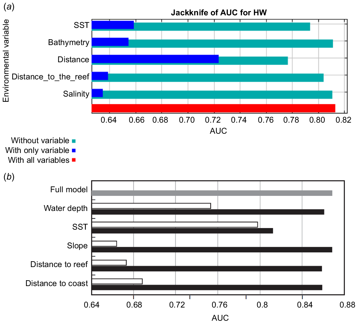
Results from the jackknife test showed that the variable that contributed the most to Smith et al.’s (2012) model was SST, followed by water depth (Fig. 7). In contrast, in Model C distance to the coast was the most important variable, followed by SST.
Results of the jackknife test of variable importance to AUC for (a) Model C and (b) Model by Smith et al. (2012). Blue/white bars represent the AUC values when each model uses only a single variable. Turquoise/black bars depict the AUC values when each model removes a single variable from the general model. Red/grey bars represent the average AUC value across all test iterations for each model.
As further validation, Model X was developed using the model settings and environmental variables (SST, bathymetry, distance to the coast, distance to the reef, and salinity) that yielded the best fit (Model C), along with an approximation of the BPC dataset used in the study by Smith et al. (2012). Model X gave approximately the same potential habitat suitability distribution (Fig. S6) and the relationship between the predicted probability of occurrence and the environmental variables (Fig. S7) as the model by Smith et al. (2012). In both models, bathymetry and SST were identified as the most important drivers according to the jackknife test (Fig. S8).
Discussion
Species distribution modelling
We developed the best-fit Maxent model for HW distribution in the GBRMP based on citizen science data using a range of bias-correction methods. We observed that areas with the highest habitat suitability for HWs were concentrated between 15 and 21°S, predominantly in the north-eastern coastal region of the GBRMP. Environmental characteristics of suitable areas suggest that high habitat suitability for HWs generally occurs in shallow (−7 m and −33 m) and warm waters (25.7–26.4°C) that are nearshore (0.24–37 km from the coast). These results are consistent with previous research, where HW showed a preference for shallow (Derville et al. 2019; Chou et al. 2020) and warm (Rasmussen et al. 2007) habitats in their breeding grounds. HWs on breeding grounds are often in nearshore waters (Thums et al. 2018; Chou et al. 2020), as we found for HWs from subpopulation E1 in the present study.
Furthermore, our findings revealed that implementing bias-correction methods improved the complexity of the SDMs, but using the spatial rarefying approach resulted in the best-fitting model. Through this process, we generated further distribution models for HW in the GBRMP and contributed to the assessment/validation of such modelling approaches. Our data indicated clustering, which is a common challenge when dealing with opportunistic sightings. Spatial rarefying removed >90% of data in datasets from both time spans. Despite the reduction in data, spatial rarefying led to improved models and produced the best-fit model (Model C). Thus, spatial rarefying is an adequately robust correction method that helps to enhance the accuracy and reliability of SDMs based on opportunistic sightings (Kramer-Schadt et al. 2013; Boria et al. 2014; Fourcade et al. 2014). However, applying bias corrections in models C – J decreased AUC scores compared to the models with no bias correction, A and B, possibly because biased data produce an elevated assessment of model performance because of the overfitting of spatially autocorrelated data (Radosavljevic and Anderson 2014). Overfitted models often generate overly complex models, which are likely to have poor predictive ability for unsampled cells and to make predictions that fit too closely to known occurrences (Peterson et al. 2011). Consequently, the observed decrease in model performance following bias correction could indicate an improvement in addressing the biases. In addition, models with bias corrections showed a more widely spread habitat suitability distribution of HW than models with no bias correction, which is also an indicator of SDM improvement.
Comparison to previous research
We compared our model output to an existing model (Smith et al. 2012), revealing a lack of fit between the two models. By utilising the model settings and environmental variables that yielded the best fit, in conjunction with an approximation of the sighting dataset used in the study by Smith et al. (2012), we constructed a model that validated our approach. Our results suggested the significance and contribution of environmental factors to a model vary when utilising different datasets.
After establishing confidence in the Maxent settings used for Model C, we compared its results with the SDM developed by Smith et al. (2012), which utilised different opportunistic data. Our findings highlight a distinct preference for the eastern coastal region of the GBRMP in Model C, whereas Smith et al. (2012) observed the highest habitat preference near the reef itself. The disparity could be attributed to the distinct spatial coverage of whale sightings by the two datasets (Fig. S9). The limitations of whale-watching excursions, where vessels have limited search time and tend to cover the same area on each trip, are likely to have led to a spatial bias in our dataset. Vessels prioritise sightings of whales closest to the harbour based on previous observations, potentially resulting in duplicated counts and clustering of sightings around nearshore areas. In comparison, BPC aerial surveillance data predominantly captures offshore reef regions.
Furthermore, the variation in temporal coverage of the data may also contribute to the discrepancy. Model C encompassed all months from 2000 to 2014, whereas Smith et al. (2012) focused solely on observations from July and August between 2003 and 2007. This limited temporal range might have resulted in fewer recorded HW sightings along the coast, potentially underestimating the suitability of this zone as a preferred habitat. An additional factor to consider is the inshore movement and increased coastal dependence of HWs, especially among calf groups, observed later in the breeding season (Smith et al. 2021). Model C sighting data covering the full breeding season provides a different perspective on HW habitat preferences, highlighting the greater coastal dependency and demonstrating the importance of considering temporal coverage when assessing HW distribution, particularly in relation to their breeding behaviours and spatial preferences.
Still, results from Model X provided evidence for the validity of our modelling techniques by predicting a remarkably similar potential habitat suitability distribution to Smith et al.’s (2012) model when using the same data, and the response curves of both models exhibited similar relationships among variables. Importantly, the jackknife test identified bathymetry and SST as the most influential drivers of the species distribution. That means the same relationship between HWs and their environment is retained when using the BPC dataset along with the environmental variables and the Maxent parameters selected for Model C. The main difference between the two models lies in the presence of larger areas with high habitat suitability in the Maxent model, indicated by the colour red in Model X (Fig. S6). This discrepancy can be attributed to the distinct set of variables employed in each model. Model X employed environmental predictors such as SST, salinity, bathymetry, distance to the coast, and distance to the reef, which aligns closely with the variables used by Smith et al. (2012). However, whereas we incorporated salinity in our model, Smith et al. opted to include seafloor slope in their analysis. This suggests that the patterns of habitat suitability for HWs are influenced by variable selection. Although salinity did not emerge as a primary driver, its presence in the model contributes to a better understanding of the marine environment by potentially capturing slight variations in habitat preferences that are not solely dictated by temperature and depth. Our decision to include salinity, given its expected significance in coastal regions, diverges from Smith et al.’s model, which excluded this variable, likely due to most of the BPC sightings being offshore. Furthermore, Smith et al.’s findings on the homogeneity of the seafloor slope and the absence of clear patterns in the response curves suggest a minimal impact on HW distribution in the GBRMP (Smith et al. 2021). Given that slope is a secondary metric derived from bathymetry (Dolan 2012), its value is limited without significant depth variations, such as those near continental shelves. This rationale guided our preference for bathymetry use over derivatives like slope or rugosity.
The high percentage of niche overlap (95%), supported by whale sightings in these areas, suggests that nearly all the environmental conditions found in the dataset employed by Smith et al. (2012) are also present in our dataset. This finding emphasises that the environmental diversity of the GBRMP is adequately represented in Model C.
Future studies, outlook, and improvements
This study demonstrates the benefits and limitations of using opportunistic data to establish habitat use by HWs. Opportunistic data are collected by non-experts, often without a clear scientific objective. Although these data sources can provide valuable information on species occurrence and environmental conditions, inadequate or biased data can result in inaccurate model predictions. For instance, the data used herein were biased towards the coast, causing our models to overestimate or underestimate the habitat suitability in other areas. Opportunistic data may be incomplete or contain errors, which can further reduce the accuracy of predictive SDMs. For example, we encountered HW sightings falling on land (incorrect longitude/latitude), duplicate data and false entries (improper data logging), and not all errors can be removed. It is further important to recognise that Maxent modelling itself also has inherent limitations. Although capable of handling opportunistic sightings and offering options to address bias through tuning, filtering, or other methods, Maxent ideally requires systematic sampling of the entire sampling domain. In many cases, including for HW sightings data, this is not the case, thereby limiting the full predictive powers of the modelling technique. Especially in the absence of sufficient spatial coverage, incorporating scientific survey data alongside citizen science data stands out as the most effective means to obtain models that closely reflect reality. This dual approach can provide a more comprehensive understanding of habitat suitability, addressing potential biases and enhancing the overall reliability of species distribution models.
Despite their limitations and biases, opportunistic data offer a wealth of information on species occurrence. With innovative approaches and careful consideration, researchers can use citizen science data to better understand and protect HWs. This collaborative approach holds immense promise for the continued conservation of HWs and their critical habitats. The findings of this study have important implications for the conservation of HWs and their habitats by shedding light on significant areas that enhance existing knowledge and support conservation initiatives in the GBRMP. For instance, the Whitsundays (part of the GBRMP) are home to HWs in the breeding season and are poised to be declared a World Whale Heritage area due to their significance (Roulston 2023). This designation highlights the need for comprehensive studies and conservation efforts in this area.
Conflicts of interest
The authors declare no conflicts of interest. No ethics approval was needed, as the research did not involve animal subjects.
Declaration of funding
This research received funding from a private charitable trust as part of the Whales and Climate Program.
Acknowledgements
The authors would like to express their appreciation to Joshua N. Smith for permission to utilise HW sightings data, which greatly contributed to the analysis presented in this manuscript. His valuable insights and feedback on earlier versions of this paper are also acknowledged. The research was supported by the Whales and Climate Program www.whalesandclimate.org.
References
Aiello-Lammens ME, Boria RA, Radosavljevic A, Vilela B, Anderson RP (2015) spThin: an R package for spatial thinning of species occurrence records for use in ecological niche models. Ecography 38(5), 541-545.
| Crossref | Google Scholar |
Atlas of Living Australia (2022) Humpback Whale – Megaptera novaeangliae [Dataset]. Atlas of Living Australia, Great Barrier Reef. Available at https://collections.ala.org.au/
Australian Marine Mammal Centre (2022) National marine mammal data portal [Dataset]. Department of Climate Change, Energy, the Environment and Water, Great Barrier Reef. Available at https://www.re3data.org/
Barbet-Massin M, Jiguet F, Albert CH, Thuiller W (2012) Selecting pseudo-absences for species distribution models: how, where and how many? Methods in Ecology and Evolution 3, 327-338.
| Crossref | Google Scholar |
Beaman R (2020) Project 3DGBR: gbr100 high-resolution bathymetry for the Great Barrier Reef and Coral Sea. Version 6 [Dataset]. James Cook University, Australia. Available at https://www.deepreef.org/2010/07/06/gbr-bathy/
Bombosch A, Zitterbart DP, Van Opzeeland I, Frickenhaus S, Burkhardt E, Wisz MS, Boebel O (2014) Predictive habitat modelling of humpback (Megaptera novaeangliae) and Antarctic minke (Balaenoptera bonaerensis) whales in the Southern Ocean as a planning tool for seismic surveys. Deep Sea Research Part I: Oceanographic Research Papers 91, 101-114.
| Crossref | Google Scholar |
Boria RA, Olson LE, Goodman SM, Anderson RP (2014) Spatial filtering to reduce sampling bias can improve the performance of ecological niche models. Ecological Modelling 275, 73-77.
| Crossref | Google Scholar |
Bouchet PJ, Thiele D, Marley SA, Waples K, Weisenberger F, Rangers B, Rangers BJ, Rangers D, Rangers NBY, Rangers NN, Rangers U, Raudino H (2021) Regional assessment of the conservation status of snubfin dolphins (Orcaella heinsohni) in the Kimberley region, Western Australia. Frontiers in Marine Science 7, 614852.
| Crossref | Google Scholar |
Brodie JE, Kroon FJ, Schaffelke B, Wolanski EC, Lewis SE, Devlin MJ, Bohnet IC, Bainbridge ZT, Waterhouse J, Davis AM (2012) Terrestrial pollutant runoff to the Great Barrier Reef: an update of issues, priorities and management responses. Marine Pollution Bulletin 65(4–9), 81-100.
| Crossref | Google Scholar | PubMed |
Brown JL (2014) SDMtoolbox: a python-based GIS toolkit for landscape genetic, biogeographic and species distribution model analyses. Methods in Ecology and Evolution 5(7), 694-700.
| Crossref | Google Scholar |
Chaloupka M, Osmond M (1999) Spatial and seasonal distribution of HWs in the Great Barrier Reef Region. American Fisheries Society Symposium 23, 89-106.
| Google Scholar |
Chou E, Kershaw F, Maxwell SM, Collins T, Strindberg S, Rosenbaum HC (2020) Distribution of breeding humpback whale habitats and overlap with cumulative anthropogenic impacts in the Eastern Tropical Atlantic. Diversity and Distributions 26(5), 549-564.
| Crossref | Google Scholar |
Clapham P (2001) Why do baleen whales migrate? A response to Corkeron and Connor. Marine Mammal Science 17(2), 432-436.
| Crossref | Google Scholar |
Craig AS, Herman LM (1997) Sex differences in site fidelity and migration of humpback whales (Megaptera novaeangliae) to the Hawaiian Islands. Canadian Journal of Zoology 75(11), 1923-1933.
| Crossref | Google Scholar |
Derville S, Torres LG, Albertson R, Andrews O, Baker CS, Carzon P, Constantine R, Donoghue M, Dutheil C, Gannier A, Oremus M, Poole MM, Robbins J, Garrigue C (2019) Whales in warming water: assessing breeding habitat diversity and adaptability in Oceania’s changing climate. Global Change Biology 25(4), 1466-1481.
| Crossref | Google Scholar | PubMed |
Devlin MJ, McKinna LW, Álvarez-Romero JG, Petus C, Abott B, Harkness P, Brodie J (2012) Mapping the pollutants in surface riverine flood plume waters in the Great Barrier Reef, Australia. Marine Pollution Bulletin 65(4–9), 224-235.
| Crossref | Google Scholar | PubMed |
Devlin MJ, Petus C, Da Silva E, Tracey D, Wolff NH, Waterhouse J, Brodie J (2015) Water quality and river plume monitoring in the Great Barrier Reef: an overview of methods based on ocean colour satellite data. Remote Sensing 7(10), 12909-12941.
| Crossref | Google Scholar |
Dickinson JL, Zuckerberg B, Bonter DN (2010) Citizen science as an ecological research tool: challenges and benefits. Annual Review of Ecology, Evolution, and Systematics 41, 149-172.
| Crossref | Google Scholar |
Dormann CF, Elith J, Bacher S, Buchmann C, Carl G, Carre G, Marquez JRG, Gruber B, Lafourcade B, Leitao PJ, Munkemuller T, McClean C, Osborne PE, Reineking B, Schroder B, Skidmore AK, Zurell D, Lautenbach S (2013) Collinearity: a review of methods to deal with it and a simulation study evaluating their performance. Ecography 36(1), 27-46.
| Crossref | Google Scholar |
Duengen D, Burkhardt E, El-Gabbas A (2022) Fin whale (Balaenoptera physalus) distribution modeling on their Nordic and Barents Seas feeding grounds. Marine Mammal Science 38, 1583-1608.
| Crossref | Google Scholar |
Elith J, Phillips SJ, Hastie T, Dudik M, Chee YE, Yates CJ (2011) A statistical explanation of MaxEnt for ecologists. Diversity and Distributions 17(1), 43-57.
| Crossref | Google Scholar |
Ersts PJ, Rosenbaum HC (2003) Habitat preference reflects social organization of humpback whales (Megaptera novaeangliae) on a wintering ground. Journal of Zoology 260(4), 337-345.
| Crossref | Google Scholar |
Esri (2021) ArcGIS Pro (Version 2.9.0) [GIS software]. Available at https://www.arcgis.com/
Eye on the Reef (2022) Eye on the Reef monitoring and assessment program [dataset]. Great Barrier Reef Marine Park Authority, Great Barrier Reef. Available at https://www2.gbrmpa.gov.au/
Fleming AH, Clark CT, Calambokidis J, Barlow J (2016) Humpback whale diets respond to variance in ocean climate and ecosystem conditions in the California Current. Global Change Biology 22, 1214-1224.
| Crossref | Google Scholar | PubMed |
Fourcade Y, Engler JO, Rodder D, Secondi J (2014) Mapping species distributions with MAXENT using a geographically biased sample of presence data: a performance assessment of methods for correcting sampling bias. PLoS ONE 9(5), e97122.
| Crossref | Google Scholar | PubMed |
Franklin T, Franklin W, Brooks L, Harrison P, Baverstock P, Clapham P (2011) Seasonal changes in pod characteristics of eastern Australian humpback whales (Megaptera novaeangliae), Hervey Bay 1992–2005. Marine Mammal Science 27(3), E134-E152.
| Crossref | Google Scholar |
Gambell R (1976) World whale stocks. Mammal Review 6(1), 41-53.
| Crossref | Google Scholar |
Geoscience Australia (2023) Maritime boundary definitions. Available at https://www.ga.gov.au/scientific-topics/marine/jurisdiction/maritime-boundary-definitions [Accessed 5 April 2024]
Gledhill DC, Hobday AJ, Welch DJ, Sutton SG, Lansdell MJ, Koopman M, Jeloudev A, Smith A, Last PR (2014) Collaborative approaches to accessing and utilising historical citizen science data: a case-study with spearfishers from eastern Australia. Marine and Freshwater Research 66(3), 195-201.
| Crossref | Google Scholar |
Gosby C, Erbe C, Harvey ES, Figueroa Landero MM, McCauley RD (2022) Vocalizing humpback whales (Megaptera novaeangliae) migrating from Antarctic feeding grounds arrive earlier and earlier in the Perth Canyon, Western Australia. Frontiers in Marine Science 9, 1086763.
| Crossref | Google Scholar |
Guidino C, Llapapasca MA, Silva S, Alcorta B, Pacheco AS (2014) Patterns of spatial and temporal distribution of humpback whales at the Southern Limit of the Southeast Pacific Breeding Area. PLoS ONE 9(11), e112627.
| Crossref | Google Scholar | PubMed |
Hijmans RJ, Garrett KA, Huaman Z, Zhang DP, Schreuder M, Bonierbale M (2000) Assessing the geographic representativeness of genebank collections: the case of Bolivian wild potatoes. Conservation Biology 14, 1755-1765.
| Crossref | Google Scholar | PubMed |
Johnston DW, Chapla ME, Williams LE, Mattila DK (2007) Identification of humpback whale Megaptera novaeangliae wintering habitat in the Northwestern Hawaiian Islands using spatial habitat modeling. Endangered Species Research 3, 249-257.
| Google Scholar |
Kadmon R, Farber O, Danin A (2004) Effect of roadside bias on the accuracy of predictive maps produced by bioclimatic models. Ecological Applications 14, 401-413.
| Crossref | Google Scholar |
Kramer-Schadt S, Niedballa J, Pilgrim JD, Schröder B, Lindenborn J, Reinfelder V, Stillfried M, Heckmann I, Scharf AK, Augeri DM, Cheyne SM, Hearn AJ, Ross J, Macdonald DW, Mathai J, Eaton J, Marshall AJ, Semiadi G, Rustam R, Bernard H, Alfred R, Samejima H, Duckworth JW, Breitenmoser-Wuersten C, Belant JL, Hofer H, Wilting A (2013) The importance of correcting for sampling bias in MaxEnt species distribution models. Diversity and Distributions 19(11), 1366-1379.
| Crossref | Google Scholar |
Kumar S, Neven LG, Zhu H, Zhang R (2015) Assessing the global risk of establishment of Cydia pomonella (Lepidoptera: Tortricidae) using CLIMEX and MaxEnt Niche Models. Journal of Economic Entomology 108(4), 1708-1719.
| Crossref | Google Scholar | PubMed |
Lindsay RE, Constantine R, Robbins J, Mattila DK, Tagarino A, Dennis TE (2016) Characterising essential breeding habitat for whales informs the development of large-scale Marine Protected Areas in the South Pacific. Marine Ecology Progress Series 548, 263-275.
| Crossref | Google Scholar |
Lysy M, Stasko AD, Swanson HK (2014) nicheROVER:(Niche)(R) egion and Niche (Over) lap metrics for multidimensional ecological niches (version 1.0). R package version 1(0). Available at https://cran.r-project.org/web/packages/nicheROVER/index.html
Mackintosh NA (1942) The southern stocks of whalebone whales. Discovery Reports 22, 197-300.
| Google Scholar |
May-Collado L, Gerrodette T, Calambokidis J, Rasmussen K, Sereg I (2005) Patterns of cetacean sighting distribution in the Pacific Exclusive Economic Zone of Costa Rica, based on data collected from 1979-2001. Revista de Biologia Tropical 53(1–2), 249-263.
| Google Scholar | PubMed |
McCulloch S, Meynecke J-O, Franklin T, Franklin W, Chauvenet ALM (2021) Humpback whale (Megaptera novaeangliae) behaviour determines habitat use in two Australian bays. Marine and Freshwater Research 72(9), 1251-1267.
| Crossref | Google Scholar |
Meynecke J-O, Richards R, Sahin O (2017) Whale watch or no watch: the Australian whale watching tourism industry and climate change. Regional Environmental Change 17(2), 477-488.
| Crossref | Google Scholar |
Meynecke J-O, Seyboth E, De Bie J, Barraqueta J-LM, Chama A, Dey SP, Lee SB, Tulloch V, Vichi M, Findlay K, Roychoudhury AN, Mackey B (2020) Responses of humpback whales to a changing climate in the Southern Hemisphere: priorities for research efforts. Marine Ecology 41(6), e12616.
| Crossref | Google Scholar |
Moua Y, Roux E, Seyler F, Briolant S (2020) Correcting the effect of sampling bias in species distribution modeling – a new method in the case of a low number of presence data. Ecological Informatics 57, 101086.
| Crossref | Google Scholar |
Muscarella R, Galante PJ, Soley-Guardia M, Boria RA, Kass JM, Uriarte M, Anderson RP (2014) ENMeval: an R package for conducting spatially independent evaluations and estimating optimal model complexity for Maxent ecological niche models. Methods in Ecology and Evolution 5(11), 1198-1205.
| Crossref | Google Scholar |
Neath AA, Cavanaugh JE (2012) The Bayesian information criterion: background, derivation, and applications. WIREs Computational Statistics 4(2), 199-203.
| Crossref | Google Scholar |
Noviello N, McGonigle C, Jacoby DMP, Meyers EKM, Jiménez-Alvarado D, Barker J (2021) Modelling critically endangered marine species: bias-corrected citizen science data inform habitat suitability for the angelshark (Squatina squatina). Aquatic Conservation: Marine and Freshwater Ecosystems 31(12), 3451-3465.
| Crossref | Google Scholar |
Ocean Biodiversity Information System (2022) Megaptera novaeangliae [dataset]. UNESCO, Great Barrier Reef. Available at https://obis.org/
Oviedo L, Solís M (2008) Underwater topography determines critical breeding habitat for humpback whales near Osa Peninsula, Costa Rica: implications for Marine Protected Areas. Revista de Biologia Tropical 56, 591-602.
| Google Scholar | PubMed |
Pacheco AS, Llapapasca MA, López-Tejada NL, Silva S, Alcorta B (2021) Modeling breeding habitats of humpback whales Megaptera novaeangliae as a function of group composition. Marine Ecology Progress Series 666, 203-215.
| Crossref | Google Scholar |
Phillips SJ (2006) A brief tutorial on Maxent. AT&T Research 190(4), 231-259.
| Google Scholar |
Phillips SJ, Anderson RP, Schapire RE (2006) Maximum entropy modeling of species geographic distributions. Ecological Modelling 190(3–4), 231-259.
| Crossref | Google Scholar |
Phillips SJ, Dudík M, Elith J, Graham CH, Lehmann A, Leathwick J, Ferrier S (2009) Sample selection bias and presence-only distribution models: implications for background and pseudo-absence data. Ecological Applications 19, 181-197.
| Crossref | Google Scholar | PubMed |
Phillips SJ, Anderson RP, Dudík M, Schapire RE, Blair ME (2017) Opening the black box: an open-source release of Maxent. Ecography 40(7), 887-893.
| Crossref | Google Scholar |
Phillips SJ, Dudík M, Schapire RE (2021) Maxent software for modeling species niches and distribution (version 3.4.4) [species modelling software]. Available at https://biodiversityinformatics.amnh.org/open_source/Maxent/
QGIS Development Team (2022) QGIS geographic information system (version 3.22.5) [GIS software]. Available at http://www.qgis.org
R Core Team (2022) R (Version 2.9.0) [Statistical software]. Available at https://www.r-project.org/
Radosavljevic A, Anderson RP (2014) Making better Maxent models of species distributions: complexity, overfitting and evaluation. Journal of Biogeography 41, 629-643.
| Crossref | Google Scholar |
Ramp C, Delarue J, Palsbøll PJ, Sears R, Hammond PS (2015) Adapting to a warmer ocean—seasonal shift of baleen whale movements over three decades. PLoS ONE 10(3), e0121374.
| Crossref | Google Scholar | PubMed |
Rasmussen K, Palacios DM, Calambokidis J, Saborío MT, Dalla Rosa L, Secchi ER, Steiger GH, Allen JM, Stone GS (2007) Southern Hemisphere humpback whales wintering off Central America: insights from water temperature into the longest mammalian migration. Biology Letters 3(3), 302-305.
| Crossref | Google Scholar | PubMed |
Ratnarajah L, Melbourne-Thomas J, Marzloff MP, Lannuzel D, Meiners KM, Chever F, Nicol S, Bowie AR (2016) A preliminary model of iron fertilisation by baleen whales and Antarctic krill in the Southern Ocean: sensitivity of primary productivity estimates to parameter uncertainty. Ecological Modelling 320, 203-212.
| Crossref | Google Scholar |
Reddy S, Dávalos LM (2003) Geographical sampling bias and its implications for conservation priorities in Africa. Journal of Biogeography 30, 1719-1727.
| Crossref | Google Scholar |
Roman J, Estes JA, Morissette L, Smith C, Costa D, McCarthy J, Nation JB, Nicol S, Pershing A, Smetacek V (2014) Whales as marine ecosystem engineers. Frontiers in Ecology and the Environment 12, 377-385.
| Crossref | Google Scholar |
Rosenbaum HC, Maxwell SM, Kershaw F, Mate B (2014) Long-range movement of humpback whales and their overlap with anthropogenic activity in the South Atlantic Ocean. Conservation Biology 28(2), 604-615.
| Crossref | Google Scholar | PubMed |
Simmons ML, Marsh H (1986) Sightings of humpback whales in Great Barrier Reef waters. Scientific Reports of the Whale Research Institution 37, 31-46.
| Google Scholar |
Smith JN, Grantham HS, Gales N, Double MC, Noad MJ, Paton D (2012) Identification of humpback whale breeding and calving habitat in the Great Barrier Reef. Marine Ecology Progress Series 447, 259-272.
| Crossref | Google Scholar |
Smith JN, Kelly N, Renner IW (2021) Validation of presence-only models for conservation planning and the application to whales in a multiple-use marine park. Ecological Applications 31(1), e02214.
| Crossref | Google Scholar |
Torre-Williams L, Martinez E, Meynecke JO, Reinke J, Stockin KA (2019) Presence of newborn humpback whale (Megaptera novaeangliae) calves in Gold Coast Bay, Australia. Marine and Freshwater Behaviour and Physiology 52(5), 199-216.
| Crossref | Google Scholar |
Tyberghein L, Verbruggen H, Pauly K, Troupin C, Mineur F, De Clerck O (2012) Bio-ORACLE: a global environmental dataset for marine species distribution modelling. Global Ecology and Ogeography 21, 272-281.
| Crossref | Google Scholar |
Ward DF (2006) Modelling the potential geographic distribution of invasive ant species in New Zealand. Biological Invasions 9(6), 723-735.
| Crossref | Google Scholar |
Warren DL, Glor RE, Turelli M (2010) ENMTools: a toolbox for comparative studies of environmental niche models. Ecography 33(3), 607-611.
| Crossref | Google Scholar |
Whitehead H, Moore MJ (1982) Distribution and movements of West Indian humpback whales in winter. Canadian Journal of Zoology 60(9), 2203-2211.
| Crossref | Google Scholar |
World Cetacean Alliance (2024) Whitsundays designated as a Whale Heritage Area - World Cetacean Alliance. https://worldcetaceanalliance.org/2024/03/25/whitsundays-designated-as-a-whale-heritage-area/ [Accessed 16 May 2024].