

Benthic communities of the lower mesophotic zone on One Tree shelf edge, southern Great Barrier Reef, Australia
Raven M. Wright A * , Robin J. Beaman B , James Daniell A , Tom C. L. Bridge A C , Jodie Pall D and Jody M. Webster D
A College of Science and Engineering, James Cook University, Townsville, Qld 4814, Australia.
B College of Science and Engineering, James Cook University, PO Box 6811, Cairns, Qld 4870, Australia.
C Biodiversity and Geosciences Program, Museum of Tropical Queensland, Queensland Museum Network, Townsville, Qld 4810, Australia.
D Geocoastal Research Group, School of Geosciences, University of Sydney, Sydney, NSW 2006, Australia.
Marine and Freshwater Research 74(13) 1178-1192 https://doi.org/10.1071/MF23050
Submitted: 9 March 2023 Accepted: 29 July 2023 Published: 24 August 2023
© 2023 The Author(s) (or their employer(s)). Published by CSIRO Publishing. This is an open access article distributed under the Creative Commons Attribution-NonCommercial-NoDerivatives 4.0 International License (CC BY-NC-ND)
Abstract
Context: Increasing interest in mesophotic coral ecosystems has shown that reefs in deep water show considerable geomorphic and ecological variability among geographic regions.
Aims: We provide the first investigation of mesophotic reefs at the southern extremity of the Great Barrier Reef (GBR) to understand the biotic gradients and habitat niches in the lower mesophotic zone.
Methods: Multibeam data were used to target five benthic imagery transects collected in the lower mesophotic (80–130 m) zone from the shelf edge near One Tree Island (23°S, 152°E) by using a single HD-SDI subsea camera.
Key results: Transects supported similar benthic communities in depths of 80–110 m, with the abundance of sessile benthos declining below ~110 m where the shelf break grades into the upper continental slope.
Conclusions: The effect of the Capricorn Eddy may be promoting homogeneity of benthic assemblages, because it provides similar environmental conditions and potential for connectivity. Variation in benthic communities between hard and soft substrate and differing topographic relief within the study site are likely to be influenced by variation in sedimentation, including sensitivity to suspended particles.
Implications: This study highlighted that the lower mesophotic region on the One Tree shelf edge supports mesophotic coral ecosystems that vary depending on depth and substrate.
Keywords: Australia, benthic communities, CATAMI, continental shelf, geomorphology, Great Barrier Reef, lower mesophotic zone, mesophotic coral ecosystems.
Introduction
Mesophotic coral ecosystems (MCEs) are low-light reef communities that occur in depths of ~30–150 m across tropical and subtropical oceans (Pyle and Copus 2019). Whereas shallow coral reefs (0–30 m) have been the topic of research for many years, comparatively fewer studies have been conducted on their deeper-water counterparts (e.g. Loya et al. 2016; Pyle and Copus 2019). The upper MCE zone (~30–60 m) exhibits high taxonomic overlap with shallow reefs; however, the proportion of shared species declines with increasing depth, particularly below ~60 m (Kahng et al. 2017; Lesser et al. 2019). The lower mesophotic zone is characterised by lower light levels and is inhabited by many deeper-reef specialists that are not found in shallow waters (Hoarau et al. 2021; Lesser et al. 2021).
The occurrence of MCEs in any particular location depends on various abiotic factors, including the presence of suitable hard substratum for benthic organisms, light penetration and water temperature (Tenggardjaja et al. 2014). Of these, one of the most important driving factors for benthic community composition is light limitation, which is observed through depth-stratification patterns (Tamir et al. 2019; Laverick et al. 2020). Depth-stratification patterns in MCEs lead to distinct but spatially variable divisions into ‘upper’ and ‘lower’ mesophotic zones (Loya et al. 2016), which are delineated by a decline in phototrophic taxa at lower mesophotic depths (Bridge et al. 2011a; Lesser et al. 2019). The upper mesophotic with raised or gently sloping hard substratum are rich in scleractinians (hard corals), soft corals and sponges that also occur among shallow reefs (Loya et al. 2016). The lower mesophotic depths and steep walls tend to be characterised by filter feeders, such as heterotrophic octocorals, black corals and sponges, with only a few deep-specialist hard coral species (Kahng et al. 2019; Hoarau et al. 2021; Pawlik et al. 2022). The lower mesophotic zone can be distinguished from true deep-sea communities by several factors, including occurring only in tropical or subtropical regions, generally residing above 200 m, and are an extension of their shallow-water counter-parts, whereas true deep-sea communities are found globally from ~200 m to the bottom of the ocean and include a much larger region by area or volume (Woodall et al. 2018).
The shift from phototroph- to heterotroph-dominated benthic communities in the central Great Barrier Reef (GBR) occurs at depths between 60 and 70 m (Bridge et al. 2011a), a pattern which is repeated in many geographic regions (Lesser et al. 2019). This transition coincides with light levels declining to <1% of surface irradiance in clear oceanic waters, but can be considerably shallower where water clarity is lower (Kahng et al. 2019). Despite this consistent general transition from phototroph- to heterotroph-dominated communities, there is variability in the taxonomic composition of MCEs within and among regions (Kahng et al. 2017). For example, lower mesophotic communities in the Indo-Pacific tend to be dominated by heterotrophic octocorals, whereas in the Caribbean they are commonly dominated by sponges (Kahng et al. 2010; Benayahu et al. 2019).
Quantifying spatial variability in mesophotic ecosystems among regions is important for understanding the mechanisms structuring ecological communities and informing conservation and management of these ecosystems. Considering the lack of research and location biases, the effects of climate change on MCEs are less clear (Hoegh-Guldberg et al. 2017; Laverick et al. 2018). Additionally, these ecosystems have been known to act as a potential refuge for shallow-water species and continue to be an important habitat for fishery species (Hoegh-Guldberg et al. 2017; Laverick et al. 2018). The importance of these deeper-water systems are just beginning to be shown through the increasing availability of technology such as remotely operated vehicles (ROVs), autonomous underwater vehicles (AUVs) and deep technical scuba diving. Nonetheless, we still lack fundamental information on mesophotic ecosystems in many geographic regions, such as sessile benthic fauna and fish community composition, and the structural processes shaping these communities (Loya et al. 2016; Williams et al. 2019). This knowledge gap includes key habitat-forming sessile taxa such as octocorals, which are abundant in the lower mesophotic (60–150 m); however, information regarding their taxonomy, ecology and evolutionary origins is largely unknown (Benayahu et al. 2019).
In recent years, multibeam bathymetry surveying has shown that submerged reefs in depths of ~30–130 m are a widespread characteristic of the outer shelf in the GBR and are occupied by mesophotic communities (Harris and Davies 1989; Abbey et al. 2011). MCEs have been examined over a length of at least 1200 km along the outer shelf of the GBR, from Raine Island in the far north (11°S) to Hydrographers Passage (20°S) in the central GBR. Lower mesophotic reefs of the northern-central GBR have been investigated using AUVs and ROVs, uncovering information regarding the composition of benthic communities and how they vary along depth and geomorphic gradients (see Bridge et al. 2011a, 2019; Englebert et al. 2017). However, no studies have examined mesophotic communities associated with the southern GBR.
Given that MCEs are widespread along the northern and central GBR shelf edge, it appears likely that MCEs would also occur on equivalent geomorphic features in the southern-most parts of the GBR. To test this hypothesis, we analysed new multibeam data and drop-camera imagery from the lower mesophotic zone (~80–130 m) on the One Tree shelf edge, lying seaward of One Tree Reef in the Capricorn-Bunker Group (~23°S, 152°E). The objectives of this study were to (1) understand depth gradients and spatial variability in the benthic communities of the lower mesophotic zone on the One Tree shelf edge, and (2) identify and map operational taxonomic units (OTUs) to classify habitat niches. This research provides important baseline information on a poorly known habitat in the Great Barrier Reef Marine Park at a time when the ecosystem is rapidly changing owing to the effects of climate change (Great Barrier Reef Marine Park Authority 2019).
Regional setting
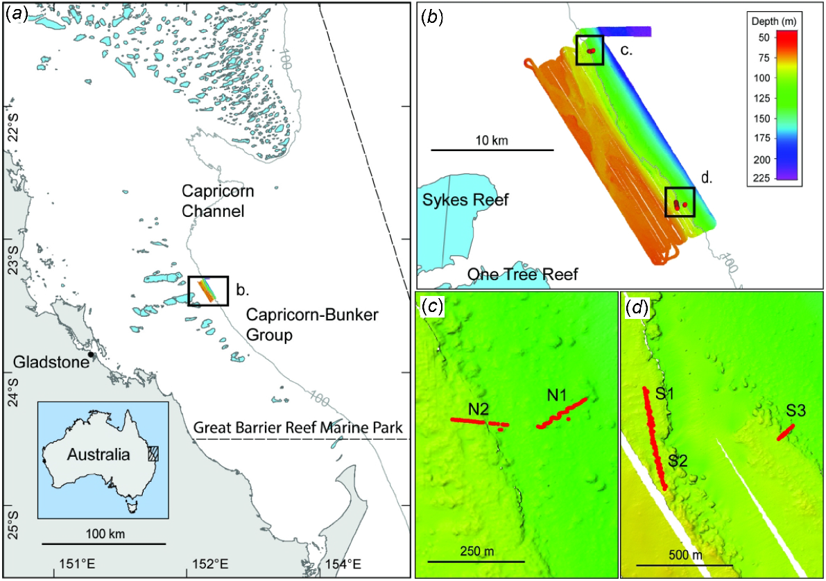
Data were collected on the R/V Sonne SO256 expedition from Auckland, New Zealand, to Darwin, Australia, via the GBR during April–May 2017 (Mohtadi et al. 2017). The One Tree shelf edge study area is located at 23°20′S, 152°10′E, ~100 km from the city of Gladstone, and lying ~10 km east of One Tree and Sykes reefs within the southern GBR Marine Park (Fig. 1). One Tree and Sykes reefs are part of the Capricorn–Bunker Group of reefs, formed mostly as a series of shallow reefs on the outer shelf. The shelf width in this region is ~90 km, with depths generally ~30–40 m to ~80 km offshore in the vicinity of the Capricorn–Bunker Group. Beyond the Capricorn–Bunker Group, depths generally drop to ~50–100 m to the limit of the shelf break. The study area also forms the south-western boundary of the prominent ~80 km wide Capricorn Channel with depths of ~80–100 m. The GBR shelf is at its widest extent north-east of the Capricorn Channel at nearly 300 km from the Australian coastline.
Maps of the One Tree shelf edge study area, showing (a) location within the southern Great Barrier Reef Marine Park; 100-m depth contour indicates the approximate shelf break; light blue polygons are the shallow coral reefs; (b) One Tree shelf edge multibeam survey ~10 km east of One Tree and Sykes reefs; (c) northern transects (Stations: N1, N2); and (d) southern transects (Stations: S1, S2, S3).
The shelf edge seaward of the Capricorn–Bunker Group of reefs has a rough topography and complex geomorphological makeup of terraces (45–175 m), notches and paleo-channels, with a smoother continental slope extending from the shelf break in depths greater than ~110 m (Veeh and Veevers 1970; Davies et al. 2004). Sweeping along the southern GBR margin, a clockwise oceanographic gyre, known as the Capricorn Eddy, is centred in the Capricorn Channel region in what is referred to as the ‘Capricorn Wedge’ (Church 1987; Weeks et al. 2010). The Capricorn Eddy and East Australian Current (EAC), which is a broader and larger southward-flowing current, have an impact on the hydrodynamics of this region, causing tidal mixing and upwelling along the shelf edge (Weeks et al. 2010; Zhibing et al. 2022). The regional subtropical climate encompasses an average sea-surface temperature of 21.5°C in the winter and 27°C in the summer, a mean yearly temperature of 24.5°C and mean annual rainfall of 1047 mm (Dechnik et al. 2015).
Materials and methods
Multibeam survey
The One Tree shelf edge study area was surveyed using a Kongsberg EM710 multibeam sonar system at a frequency of 70–100 kHz, together with surface-collected and water column-modelled sound speed profiles used to calibrate depth determination (Fig. 2a). Systematic survey line spacing was conducted between 250 and 350 m apart with a ±60° angular swath applied to collect both bathymetry and backscatter (amplitude) data. Raw Kongsberg .all files were post-processed in CARIS HIPS and SIPS software (ver. 10.4, see www.teledynecaris.com) to apply predicted tide corrections from the nearest tidal port (Heron Island, 20 km away), reducing the bathymetry data to a lowest astronomical tide (LAT) vertical datum. Manual editing was conducted as 3-D point clouds to remove any obvious noise spikes. The accepted bathymetry data were then used to develop a 2-m resolution CARIS Spatial Archive (CSAR) raster file. The CSAR raster file was interpolated twice to fill in minor data gaps, then exported as an ASCII xyz file. The xyz file was imported into QPS Fledermaus (ver. 7.8, see www.qps.nl) software to generate an equivalent 2-m resolution bathymetry grid. Fledermaus software was also used to convert the bathymetry grid into a hillshaded geotif and ESRI raster grid for further examination in ArcGIS software (ver. 10.3, see www.esri.com). The multibeam backscatter data were processed using QPS FMGeocoder Toolbox (ver. 7.10, see www.qps.nl) and gridded into a 2-m resolution image mosaic, then exported as a geotiff image for viewing in ArcGIS (Fig. 2b).
Three dimensional (3-D) view of One Tree shelf study area. (a) Bathymetry map at 2-m resolution. Depth contours in metres. (b) Relative backscatter map at 2-m resolution with the same contours. Sample sites (red lines) were taken over rough ground (lighter backscatter) features at the shelf edge. Note transition beyond shelf edge to the relatively smooth upper slope (darker backscatter).

Drop camera
Drop-camera video imagery of the seafloor was captured at transect stations from the northern and southern ends of the One Tree shelf edge study area in depths of 80–130 m (Table 1). The German company iSiTEC GmbH provided the subsea video transmission system used onboard the R/V Sonne. The single HD-SDI subsea camera was mounted on a multi-core (MUC) sediment-sampler device in a downward-looking orientation. The camera provided HD (1920 × 1080 pixels) video signals linked to the ship by fibre-optic cable that was spliced into the main winch cable for the MUC. The MUC was also equipped with two SeaLite Sphere 5150 LED lights to illuminate the seafloor, one depth sensor and one positioning sensor, together with an iXblue Posidonia ultra-short baseline (USBL) for the relative position of the MUC to the vessel. The drop camera was used similar to a towed camera, in that video footage was allowed to stream as the R/V Sonne drifted along the transect. Calibrated lasers, typically used to estimate organism size, were not used nor available in this study. Imagery had both ship position and depth, MUC position and depth, and timestamps embedded on the video imagery. Sediment coring did not occur while the video imagery was being acquired.
| Station | Start | End | Depth range (m) | Duration | Distance (m) | Total images | Classified images |
|---|---|---|---|---|---|---|---|
| N1 | −23.312563 | −23.3119187 | 114–129 | 22 min 10 s | 134 | 1330 | 65 |
| 152.128955 | 152.130074 | ||||||
| N2 | −23.3124005 | −23.3125168 | 89–112 | 24 min 08 s | 132 | 1448 | 37 |
| 152.126945 | 152.128231 | ||||||
| S1 | −23.4258625 | −23.4280072 | 83–89 | 30 min 50 s | 249 | 1850 | 76 |
| 152.192352 | 152.192684 | ||||||
| S2 | −23.4281035 | −23.4305145 | 80–89 | 32 min 24 s | 273 | 1944 | 81 |
| 152.192683 | 152.193261 | ||||||
| S3 | −23.4281487 | −23.427525 | 90–105 | 19 min 24 s | 98 | 1164 | 35 |
| 152.19861 | 152.199299 |
Five camera transect targets were selected from the multibeam bathymetry data to cross the shelf edge terrain, while the vessel was drifting at a speed of <1 knot (~1.85 km h−1). The camera was manually lowered and raised as the vessel drifted, while monitoring the live video feed, and generally flown at ~30–40 m above the seafloor, then zoomed in, to bring the seafloor into focus. The video footage varied between 19 and 32 min, with transect distances ranging between 98 and 273 m (Table 1). The relatively high altitude was possible because water clarity was very clear at the study site, and the LED lights provided sufficient illumination of the benthos beneath the camera. Two transect stations were collected in the northern end of the study area (N1, N2), and three transect stations were in the southern end of the study area (S1, S2, S3), separated by a distance of ~14 km.
The drop-camera imagery from the R/V Sonne SO256 voyage was acquired opportunistically because this was the first test of the newly installed subsea camera system mounted on the MUC device. In addition, the seafloor morphology was unknown prior to the multibeam survey and, therefore, we were unable to develop the rigorous sampling design prior to deployment, soon after the completion of the multibeam survey. Transect stations were also limited by operational constraints such as the need to drift with current and wind. Because the MUC camera was deployed (lowered) on the shelf itself and always on the landward, shallower side of the shelf, transect stations typically resulted in a skewed higher number of photo samples taken in the shallower depth categories. For example, depth category 1 (80–89 m) had a significantly higher sampling rate (i.e. more images) than did the other depth categories (>89 m). Transect station S3 was also shorter than other transects, and N2 and S3 had nearly half the number of classifiable images of those of the rest of the stations. This survey was an exploratory study without a robust experimental design; therefore, it was not feasible to adhere to Australian national standard guidelines for marine monitoring. Despite these limitations, the data collected represent the first opportunity to examine MCEs in the lower mesophotic zone near the southern limit of the GBR, a previously unexplored region.
Image analysis
Video files were converted into still-frame photographs by using FreeStudio (ver. 5.0, see www.dvdvideosoft.com) at a 1-s interval for an output of 7736 total images across all transects. Each 1920 × 1080 pixel image had an approximate spatial footprint size of 3–4 m (width) × 1.7–2.3 m (height). After visually inspecting each image, 2071 photographs were removed from subsequent analysis because of poor image quality, either because the camera malfunctioned or the camera was too close to or too far from the seafloor. After removing unsuitable images, there were 5665 acceptable photos available for analysis.
The 5665 photographs were subsampled to analyse changes in benthic community composition along each transect. Every 10th to 20th photo, representing approximately one image every 3–5 m at a drift speed of ~0.2–0.6 knots (~0.4–1.1 km s−1), was analysed for a total of 290 images. This image distance was chosen to reduce spatial overlapping and pseudo-replication of the data extracted from each subsampled image, and to give flexibility in choosing an image with the best resolution, given the variation in image quality along each transect (Bridge et al. 2011a). The horizontal positions of each subsampled image were taken from the MUC-mounted USBL positions embedded on the selected images. Several image positions diverged up to ~15 m away from the general line trend of the transects, but most image positions were stable and followed the general line trend. We estimate that the horizontal position uncertainty of images is <2 m and thus images accurately align with the underlying bathymetry data.
The 290 photos were manually classified using a morphology-based approach, as described below (Supplementary Fig. S1, S2). Benthic fauna occurring in each of the subsampled images were scored using the five-point field-of-view percentage-coverage method for relative abundance, as outlined in Done (1982). This technique allows for every organism to be classified or accounted for on the basis of the relative abundance in the frame on a scale of 0–5 (0 = 0%, 1 = 1–5%, 2 = 6–10%, 3 = 11–30%, 4 = 31–80%, 5 = 81–100%). This method was chosen because it provides a way to rapidly quantify the community, while also recording rare taxa, which are often overlooked using methods such as random-point overlay (see Bridge et al. 2011a). The capacity to accurately identify sessile megabenthic invertebrates varies among taxa, but often requires examination of anatomical characters that are often not visible in benthic images. Therefore biota in images were identified into morphotypes by using the collaborative and automated tools for analysis of marine imagery (CATAMI) scheme, which was specifically developed to analyse benthic imagery where accurate identifications on the basis of taxonomy are not realistically achievable (Althaus et al. 2014). The morphotype approach allows categories to include both morphological and taxonomic information, thereby providing flexibility in terms of the criteria used to determine classes. Given that the categories recorded in this study represent a mix of morphological and taxonomic data collected at different taxonomic levels, we refer to each individual category as an ‘operational taxonomic unit’ (OTU) rather than a ‘taxon’.
The term OTU has been used differently in different fields, and whereas first popularised in the field of molecular biology to refer to a series of closely related sequences or taxa within a phylogeny (He et al. 2015), it is increasingly used for analysis of benthic images to delineate groups of organisms that share particular characters but are not identifiable to a particular taxonomic level (e.g. Jansen et al. 2018; Howell et al. 2019; Horton et al. 2021; Untiedt et al. 2021). CATAMI is a classification scheme that is flowchart-based, allowing for universal labelling regardless of ecosystem (i.e. shallow to abyssal), and encompasses descriptions for both biota and physical seabed properties (Althaus et al. 2014). Therefore, CATAMI provides the flexibility to enable analysis of communities where different taxa can be identified to different taxonomic levels. Despite the inherent difficulties with identification of benthic taxa from these images, we attempted to identify biota to the lowest taxonomic level possible (see Table S1). Appropriate field guides were used where available (e.g. Fabricius and Alderslade 2001), while other groups, such as hard corals, sponges and black corals, were identified with reference to relevant literature and through assistance from taxonomic experts. The physical substrate (hard or soft), relief of substrate (flat or low-moderate) and bioturbation (presence or absence) for each image was also classified on the basis of the CATAMI scheme (Fig. 3, Table 2).
Image examples of substrate, relief and other environmental variables defined by the CATAMI system. See Table 2 for descriptions. (a) Unconsolidated (soft): sand; (b) consolidated (hard): cobbles; (c) consolidated (hard): rock; (d) biogenic: rhodoliths; (e) bioturbated; (f) relief: flat; and (g) relief: low–moderate. Image dimensions ~3–4 m (width) × 1.7–2.3 m (height). Note: footage was illuminated by 2 LED lights. The colouration seen in the images illustrates the vibrant and natural colouration of these MCE communities.

| Variable | Description |
|---|---|
| Unconsolidated (soft): sand | Grain sizes defined as <2 mm in diameter |
| Consolidated (hard): cobbles | Rocks that are ~65–255 mm in size |
| Consolidated (hard): rock | Visible bedrock, outcropping ledge, or cliff face. Can be covered in biota or a sediment |
| Biogenic: rhodoliths | Substrate composed of rhodoliths, either dead or alive |
| Bioturbated | Traces or tracks formed in soft-sediment habitats by biological activity |
| Relief: flat | Flat substrate, no features |
| Relief: low-moderate | Features with a maximum height of <3 m |
Spatial variability
Depth stratification of the mesophotic benthic community was tested using the Jaccard index of dissimilarity (based on presence or absence) by measuring the changes in the CATAMI OTUs for every 10-m depth interval covered by the transects (Englebert et al. 2017). The following five depth categories were defined in 10-m increments: (1) 80–89 m, (2) 90–99 m, (3) 100–109 m, (4) 110–119 m, and (5) 120–129 m. The Jaccard index was run with all substrate types for the five depth categories, and then separately for hard substrate and soft substrate. Hard and soft substrate were compared to investigate the influence of substrate type on benthic communities. Multidimensional scaling (nMDS) was then used to analyse the associations and spatial variance among the depth categories, and also among the five different stations. OTUs were input to a Bray–Curtis matrix for relative abundance from the 290 classified images. All statistical analyses were analysed in R software (ver. 3.5.3, R Foundation for Statistical Computing, Vienna, Austria, see https://www.r-project.org/), using the packages ‘vegan’ (ver. 2.5-7, J. Oksanen, F. G. Blanchet, M. Friendly, R. Kindt, P. Legendre, D. McGlinn, P. R. Minchin, R. B. O’Hara, G. L. Simpson, P. Solymos, M. H. H. Stevens, E. Szoecs and H. Wagner, see https://cran.r-project.org/package=vegan/) and ‘ggplot2’ (ver. 4.1.3, see https://CRAN.R-project.org/package=ggplot2; Wickham 2016).
Habitat classification
Hierarchical clustering analysis was performed on 14 new OTU groupings by using the CATAMI scheme to distinguish qualitatively important seabed habitats. New groupings were made on the basis of a broader taxonomic classification so as to eliminate categories with a negligible amount of data and meet assumptions of the statistical analysis. A Euclidean distance matrix was applied alongside Ward’s method (R package ‘ward.D2’) and validated internally with the R package ‘clValid’ (ver. 4.1.3, see https://cran.r-project.org/package=clValid; Brock et al. 2008). Relative abundance averages for each of the OTU groups were calculated within each cluster to compare the organisation of biotic assemblage make-up. The new OTUs were mapped into geographic space in ArcMap and overlaid on the 2-m bathymetry grid data and backscatter mosaic. The environmental variables obtained from imagery annotation (substrate type, relief and bioturbation) were then added to the map (Fig. S3).
Results
Multibeam survey
The systematic multibeam survey conducted on the One Tree shelf edge covered an area of ~18 km long × 6 km wide (Fig. 1b, 2). Depths within the surveyed area generally range from ~40 to 200 m. The shelf break is a distinct step of ~10-m height near the 100-m contour and is non-linear because of the lobes of sediment and small promontories of hard ground and numerous low (<5 m high) pinnacles. These pinnacles continue up to ~120-m depth contour, over a horizontal distance of between 300 and 1000 m to seaward of the shelf break (Fig. 2). From ~120 to 200 m on the upper continental slope, the seabed becomes relatively smooth as the pinnacles disappear.
Present on the shelf are at least five distinct terraces at depths of ~62–65, 70, 75–80, 85, 90 and 100–105 m. In the southern section, all terraces are easily distinguishable and appear to follow contours. The terraces between 75- and 90-m depth are linear and generally unbroken across the entire study area, yet the 62–65-, 70- and 85-m terraces, while being well-defined, are non-linear. The 62–65 and 70-m terraces exhibit raised rims and are non-continuous, becoming irregular in areas incised by paleo-channels. These uppermost terraces have rough-textured surfaces owing to numerous, 1-m-sized mounds and, less commonly, merged pinnacle ridges developing on the seaward rim. The 80- and 90-m terraces also exhibit seafloor roughness in the north, whereas in the south they are noticeably smooth, reflecting sediment cover on the basis of the backscatter imagery. The 100–105-m terrace is the most prominent and widest terrace, stretching up to 780 m wide in places, although, more commonly, being less than 700 m wide. Pinnacle formation on this lower-most terrace explains the high rugosity observed in backscatter imagery.
Across the 65-m terrace, the shelf dips regionally at an average angle of ~0.2° in the north, steepening to an average angle of ~0.13° in the central section and shallowing again to ~0.05° in the south. Across the lower terraces, between the 70-m terrace and shelf break, the angle of the shelf increases from 0.8° in the north, to a relatively steep ~2.2° in the central section, and 1.1° in southern region. This indicates that terraces are more closely spaced in the southern and central sections than in the north, where terraces are up to 1 km apart. Beyond the shelf break, the outer slope shows a marked increase in downward slope angle, which varies on average between ~3.1° in the north, 1.8° in the centre and 2.8° towards the south.
A ~500 m wide, relatively low-relief channel cuts through the uppermost terraces in the centre of the survey area, highlighting a prominent paleo-channel. Backscatter imagery shows low acoustic reflectivity between the 65- and 70-m terraces, suggesting thick sediment cover. By contrast, high acoustic reflectivity on the tops of the 65-m terraces in the north and centre indicates hardground. The sediment-covered paleo-channel is at a relative topographic low (dropping between 1 and 5 m below the surrounding terraces in the north, and below 4–8 m in the centre), with gradients of between 1 and 10° where the elevated terraces meet the channel bed. Overall, the sediment deposits within the channel are smooth and, in some areas, exhibit distinct dune and ripple structures. Interruptions in the shelf break also appear to be due to paleo-channel incision, especially in the south.
Depth and biota gradients
Overall, 34 CATAMI morphological groups were identified from the five camera transect stations (N1, N2, S1, S2 and S3) in depths of 80–129 m (Table 3). The composition of living biota did not vary significantly from 80 to 109 m as the depth (categories 1–3) encompassed similar ratios of shared OTUs. However, a break in community composition occurred at 110–119 m (category 4), with even greater dissimilarity at 120–129 m (category 5; Table S2). Note the depth category 4 (110–119 m) and depth category 5 (120–129 m) were not sampled in the southern transects, owing to the opportunistic nature of the survey. Depth category 5 (120–129 m) was most dissimilar in the ratio of OTUs compared with the other depth categories (1–4) for all substrate types, reflecting where transects had crossed from the shelf break onto the upper continental slope. There was also a significant difference between hard and soft substrate, with most OTUs being found on either rock or cobble (hard) substrate, and only a few on (soft) sand.
| Morphology category | Taxa included |
|---|---|
| Stony coral: branching (11 290912) | Dendrophyllia |
| Stony coral: foliose/plate (11 290907) | Leptoseris |
| Stony coral: solitary (11 290901) | ID unknown (multiple taxa) |
| Stony coral: massive (11 290906) | ID unknown |
| Hydrocorals: branching (11 077906) | Stylaster |
| Hydroids (11 001000) | ID unknown |
| Black coral: whip (11 168917a) | Antipathidae |
| Black coral: bushy (11 168908a) | ID unknown |
| Black coral: fern-frond (11 168913a) | ID unknown |
| Black coral: arborescent (11 168904a) | Aphanipathidae (Aphanipathes?), Myriopathidae (Myriopathes?) |
| Octocoral: whip (11 168917b) | Junceella, Viminella |
| Octocoral: fleshy arborescent (11 168911b) | Nephtheidae, Chironephthya |
| Octocoral: non-fleshy arborescent (11 168904b) | Ellisella, Ctenocella, Jasminisis, ID unknown (multiple taxa) |
| Octocoral: non-fleshy bushy (11 168908b) | ID unknown (multiple taxa) |
| Octocoral: bottlebrush (11 168905b) | ID unknown |
| Octocoral: fern-frond (11 168913b) | ID unknown |
| Octocoral: fan 2-D rigid (11 168916b) | Annella, Muricella, Paracis, other Plexauridae, Muricea, non-encrusting Anthothelidae, Plumigorgia, ID unknown (multiple taxa) |
| Sponge: encrusting (10 000902) | ID unknown (multiple taxa) |
| Sponge: massive simple (10 000904) | ID unknown (multiple taxa) |
| Sponge: massive ball (10 000905) | ID unknown (multiple taxa) |
| Sponge: massive cryptic (10 000908) | ID unknown |
| Sponge: barrels (10 000907) | ID unknown |
| Sponge: tubes and chimneys (10 000911) | ID unknown (multiple taxa) |
| Sponge: stalked (10 000906) | ID unknown |
| Sponge: cup-likes (10 000910) | Carteriospongia |
| Sponge: erect branching (10 000915) | ID unknown (multiple taxa) |
| Sponge: erect simple (10 000916) | ID unknown (multiple taxa) |
| Foraminifera | Cycloclypeus carpenteri |
| Colonial anemones: zoanthids (11 284000) | ID unknown (multiple taxa) |
| Macroalgae: encrusting red (80 300934) | crustose coralline algae, rhodolith beds, Peyssonnelia |
| Macroalgae: articulated calcareous red (80 300913) | ID unknown |
| Macroalgae: articulated calcareous green (80 300912) | ID unknown (multiple taxa) |
| Macroalgae: laminate brown (80 300919) | Lobophora? |
Numbers shown in parentheses in the Morphology category column are CATAMI-specific ID numbers.
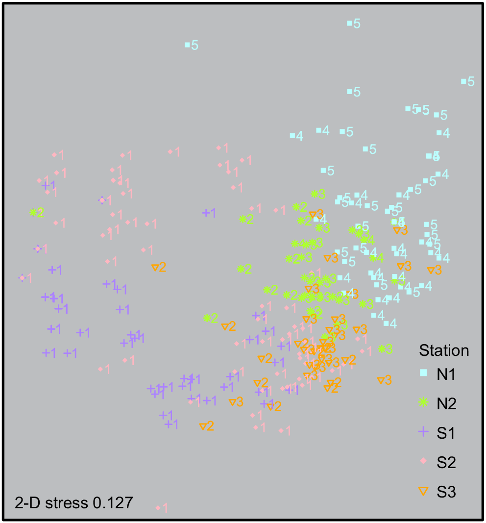
The multidimensional scaling (2-D stress = 0.127) plot shows comparable patterns with regard to depth categories 1, 2 and 3 plotting around each other; however, there is a slight separation of the grouping for stations S1 and S2 within the shallowest depth category 1 (80–89 m) to the left of the plot (Fig. 4).
Substrate and associated communities
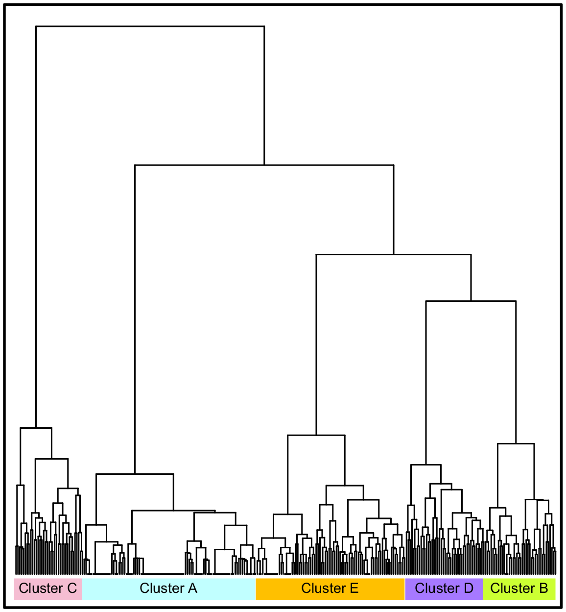
Hierarchical cluster analysis generated five clusters from the benthic data observed at the One Tree shelf edge study area (Fig. 5, Table 4).
Hierarchical cluster analysis encompassing CATAMI OTUs shown in Table 4. Cluster A is found on sandy inter-reefal habitat; Cluster B on flat sand-covered rock; Cluster C on protruding rock; Cluster D on deep rocky outcrops; and Cluster E on deep barren rock.
| OTU | Cluster A | Cluster B | Cluster C | Cluster D | Cluster E |
|---|---|---|---|---|---|
| Stony coral | 0.01 | 0.13 | 1.03 | 0.72 | 0.22 |
| Hydrozoa | 0.15 | 0.10 | 0.49 | 0.53 | 0.33 |
| Black coral | 0.02 | 2.51 | 5.27 | 1.37 | 0.12 |
| Fan gorgonians | 0.02 | 1.15 | 2.05 | 1.79 | 0.57 |
| Octocoral (all others) | 0.04 | 1.30 | 2.76 | 2.56 | 0.30 |
| Sponge (encrusting) | 0.00 | 0.33 | 2.08 | 1.70 | 0.88 |
| Sponge (massives) | 0.35 | 0.74 | 2.00 | 1.28 | 0.48 |
| Sponge (cups) | 0.02 | 0.21 | 0.46 | 0.30 | 0.01 |
| Sponge (simple) | 0.26 | 1.21 | 1.62 | 0.95 | 0.09 |
| Sponge (all others) | 0.00 | 0.08 | 0.43 | 0.02 | 0.02 |
| Zoanthid | 0.02 | 0.18 | 0.11 | 0.16 | 0.05 |
| Algae (encrusting red) | 0.01 | 0.67 | 3.03 | 3.42 | 2.75 |
| Algae (all others) | 0.04 | 0.07 | 0.43 | 0.70 | 0.28 |
| Giant foraminifera | 1.36 | 1.46 | 1.11 | 1.07 | 0.23 |
Numbers highlighted in bold indicate majority of cluster makeup.
Cluster A, i.e. sandy inter-reefal, occurred exclusively on flat, soft substrate (sand) with extensive bioturbation. It was mostly present within depth category 1 and included hydrozoa, massive sponges, simple sponges and giant foraminifera (Fig. 6a, b). Cluster B, i.e. flat sand-covered rock, comprised mostly hard substrate with mainly flat relief, although some low–moderate relief was present. Mild bioturbation was observed with a majority of the cluster being found within depth category 1. This cluster incorporated a high abundance of black coral, fan gorgonians, other octocoral, simple sponges and giant foraminifera (Fig. 6c). Cluster C, i.e. protruding rock, occurred on hard substrate with mainly low–moderate relief within depth categories 1, 2 and 3. Hard substrate was protruding rock that was not buried beneath a sandy veneer such as Cluster B, and had scarce bioturbation. Black coral, fan gorgonians, other octocoral, encrusting sponges and encrusting red algae made up the vast majority of biota in Cluster C (Fig. 6d).
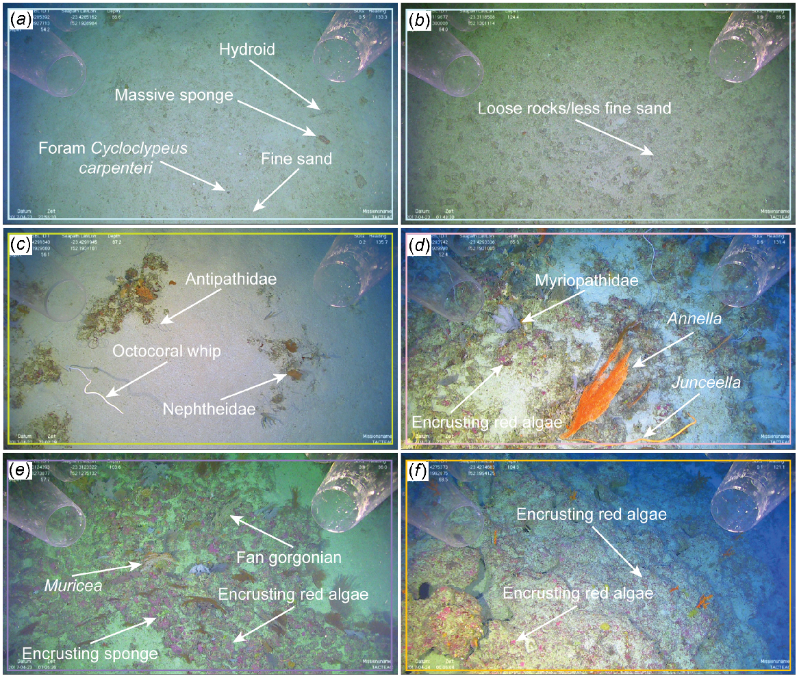
Representative images from each of the following five clusters from the One Tree shelf study area: (a) Cluster A (sandy inter-reefal) depth category 1 includes hydroids, massive and simple sponges, giant foraminifera; (b) Cluster A (sandy inter-reefal) depth category 5 on the upper slope has loose rocks and less fine-grain sand than on sandy inter-reefal on the shallower shelf; (c) Cluster B (flat sand-covered rock) depth category 1 includes black coral, fan gorgonians, erect simple sponges, giant foraminifera, other octocorals; (d) Cluster C (protruding rock) depth category 1 includes black corals, fan gorgonians, other octocorals, encrusting sponges, encrusting red coralline algae; (e) Cluster D (deep rocky outcrops) depth category 3 includes fan gorgonians, other octocorals, encrusting sponges, encrusting red coralline algae; and (f) Cluster E (deep barren rock) depth category 3 includes encrusting red coralline algae. The colour frames on each panel represent the same coloured cluster as seen in Fig. 5. Image dimensions are ~3–4 m (width) × 1.7–2.3 m (height).
Clusters D and E were generally found deeper and located in all but depth category 1. Cluster D, deep rocky outcrops, occurred exclusively on hard substrate with low–moderate relief. No bioturbation was observed within this cluster. Hard substrate was primarily rocky outcrops with large cobble patches nearby within depth categories 2, 3 and 4. A majority of the benthic fauna was composed of fan gorgonians, other octocoral, encrusting sponges, and encrusting red algae (Fig. 6e). Cluster E, i.e. deep barren rock, was the deepest cluster appearing only within depth categories 3, 4 and 5. Substrate was mostly hard, usually low–moderate relief, with flat relief where rhodolith beds were present. The rest of the hard substrate had abundant open space and no bioturbation. Encrusting red algae was the only biota found in high abundance (Fig. 6f). Stony coral, cup-like sponges, other sponges, zoanthids and all other algae did not make up a high abundance in any of the clusters and were present only in relatively small quantities compared with dominant taxon groups.
Along with biota, variables such as substrate type, relief and bioturbation were incorporated into classifying the habitats. Of these variables, hard substrate and low–moderate relief were associated with a higher mean abundance of structurally complex groups such as fan gorgonians, other octocorals and black coral being present within the clusters. The five clusters were found at most stations, thus suggesting a lack of spatial variability between benthic communities at the northern and southern One Tree shelf edge, despite a horizontal distance of ~14 km.
Discussion
The shallower portion of the lower mesophotic zone (80–109 m) of the One Tree shelf edge supported relatively homogeneous biota across the entire study area. As in more northern regions of the GBR, azooxanthellate octocorals (whip, fleshy arborescent, non-fleshy arborescent, non-fleshy bushy, bottlebrush, fern frond and fan 2-D ridge) were the most abundant OTUs in the lower mesophotic zone. Other common benthic organisms in the lower mesophotic on the One Tree shelf edge were algae, sponges and black corals, indicating that the composition of lower mesophotic communities at low taxonomic resolution in this region is similar to that in other areas of the GBR and across the wider Indo-Pacific (Loya et al. 2016; Bridge et al. 2019). Black corals, a widespread but data-deficient group, were common within our study site, and included whip, bushy, fern-frond and arborescent morphologies. Several families of black coral are common in the mesophotic zone, including Antipathidae, Aphanipathidae and Myriopathidae (Bo et al. 2019), and recent taxonomic research has shown that the diversity of black corals in north-eastern Australia is far greater than was previously thought (Horowitz et al. 2022).
Sponge density (defined by percentage cover, or relative abundance in this study) was high (appearing in ~77% of analysed images), with the most abundant types being encrusting, massive, and erect (simple and branching) sponges. Sponge density increases from shallow reefs into MCEs in both the Caribbean and Pacific, likely owing to differences in resource availability and ability to utilise resources among depths (Lesser and Slattery 2018). Macroalgae and sponges are the least studied benthic groups among mesophotic reefs, despite often being abundant (Bridge et al. 2019). Despite the lack of data from shallower depths to compare sponge density on the One Tree shelf edge, our results confirmed that the lower mesophotic zone hosts a diverse assemblage of sponges encompassing at least 10 different morphologies. Sponges can vary considerably in morphology and identification of species requires detailed examination of specimens and molecular analysis (Bell and Barnes 2000). Schönberg (2021) conducted a study on sponge functional morphology and concluded that growth forms are likely to be a response to waterflow and turbidity, reflecting ambient conditions in those regions. Although this study did not capture flow regime or sedimentation, future studies would benefit from studying the correlation between these environmental variables and sponge morphologies in the southern GBR.
Red algae was abundant in this study, supporting the hypothesis that crustose coralline algae (CCA; e.g. Peyssonnelia) and rhodoliths are predicted to occur throughout the entirety of the GBR (Abbey et al. 2013). Rhodolith beds on the One Tree shelf edge were found mainly from 100 to 130 m, and CCA were the most abundant biota observed in the images spanning the full 80–130 m depth range and were found on all hard substrates. An earlier study by Davies et al. (2004) also found that coralline algal build-ups from 80 to 120 m were present around the Capricorn–Bunker Group region and had formed during the Holocene.
Zooxanthellate scleractinia and octocorallia were rare on the One Tree shelf edge. Nonetheless, some phototrophic stony corals and octocorals were found in the lower mesophotic zone, comprising typical lower mesophotic taxa such as Leptoseris and Plumigorgia. Other CATAMI morphology groups, such as solitary and massive corals, were also observed, but could not be identified to species. Leptoseris is common in many Indo-Pacific MCEs, even at depths beyond 60 m because of its enhanced photosynthetic capacity, unique Symbiodinium host–symbiont specialisation and physiological adaptions (Pochon et al. 2015). Leptoseris has been found as deep as 125 m in the northern GBR (Englebert et al. 2015) and in the southern GBR, sparsely, as a cave-dwelling coral around the Capricorn–Bunker Group recorded from 4 to 21 m (Dinesen 1982). In contrast, little is known about Plumigorgia, other than that it is probably zooxanthellate and reportedly common on mid- and outer-shelf reefs in shallow and flow-exposed habitats of the GBR (Fabricius and Alderslade 2001).
The photosynthetic ability of zooxanthellate corals diminishes with an increasing depth and colonies start to exhibit resource partitioning (Muscatine et al. 1989). An increased capacity for heterotrophic feeding or enhanced photosynthetic abilities (i.e. mixotrophy) could explain how Plumigorgia survives in the lower mesophotic zone and why it would be common in flow-exposed environments. The velocity of the East Australian Current (EAC) has a seasonal variation (from 27.4 Sv in winter to a maximum 36.3 Sv in summer, where the unit Sv is the sverdrup, an oceanographic unit of volumetric flow rate, which is equivalent to 1 × 10⁶ m3 s) with a subsurface maximum flow that dominates down to ~150-m depth and is strongest (southward) along the GBR continental shelf (Church 1987; Ridgway and Godfrey 1997; Sloyan et al. 2021), thus exhibiting a positive flow-exposed environment within this study site. This is further supported by the fact that some habitats along the One Tree shelf edge lack sediment, indicating their exposure to significant bottom currents. Additionally, it supports the idea that Plumigorgia could be facultatively zooxanthellate, meaning it supports symbionts in shallow water, but not in deeper water (Schubert et al. 2017).
Irradiance levels, water clarity and water motion are important abiotic factors that influence the composition of benthic communities (Leichter and Genovese 2006; Kahng et al. 2010; Loya et al. 2016). Sediment ripples were observed throughout the images where soft sediment was present, indicating that the One Tree shelf edge is subjected to bottom currents despite being well below incident wave base. Meandering EAC surface currents running south from 14 to 24°S indicate a flow of up to 0.8 m s−1, with a 20–30% stronger inflow down to 200 m (Church 1987). Rapid fluctuations in temperature, nutrients and suspended particles are created by strong internal wave energy (Leichter and Genovese 2006). These environmental factors have been previously observed at other areas on the GBR outer shelf farther north of this study area (Bridge et al. 2019). During the present study, the water clarity at One Tree shelf edge was much clearer than at other sites visited during SO256, such as the Swain Reefs, which lies east of the Capricorn Channel and was very turbid in the drop-camera imagery.
The Capricorn Eddy is a major oceanographic feature that forms a stable cyclonic eddy along the southern GBR margin (Weeks et al. 2010). It has a large influence over physical properties on coral reefs located near the Capricorn Channel and surrounding areas by creating upwelling, which brings in cooler, nutrient-rich water that promotes fast growth, increases stability and promotes connectivity among reefs (Andrews and Gentien 1982; Thomas et al. 2014). This eddy is likely to have an impact the One Tree shelf edge and results in relatively homogenous oceanographic conditions across the study area. Unfortunately, no CTD deployments were conducted on the voyage for this particular site, but it is likely that the upwelling, or otherwise prevailing conditions forced by the Capricorn Eddy, could influence benthic communities on the One Tree shelf.
Topography, tidal motion, wind and oceanographic currents control the water circulation. This helps regulate connectivity within reef ecosystems and contributes to spatial heterogeneity of benthic ecosystems, particularly from the South Equatorial Current (SEC), which turns into the EAC (Lambrechts et al. 2008; Bridge et al. 2019). Whereas larger circulation processes such as the EAC potentially create a gradient of distinct communities across the whole GBR margin, local circulation is presumably controlling the environmental setting around the One Tree shelf edge (i.e. Capricorn Eddy). In this study, the absence of variability in OTUs between northern and southern stations in the shallower depth categories (80–109 m) means that connectivity is likely to be present at least at scales of tens of kilometres along the One Tree Shelf edge. Despite the lack of comparison for the deeper categories 4 and 5 (110–129 m) between the northern and southern sites, it is predicted that OTUs for deeper depths also lack variability across the One Tree shelf edge and onto the upper slope. This is based on similar depths and geomorphology as observed in multibeam data at the northern and southern stations, i.e. non-linear shelf break as a distinct step near the 100-m contour, scattered with lobes of sediment and numerous low pinnacles, becoming more smooth with distance across the upper slope.
At a finer-scale, and within the transects themselves, a distinct variation in community composition was observed depending on substrate, slope and depth. Our analysis showed clear differences in benthic communities between hard and soft substrate, whereas communities on hard substrate were further divided depending on the angle of the substrate. Sediment influences biological associations, often contributing to variation in community assemblages among substrate types, sediment particle size and chemical composition (Weinstein et al. 2015). A comprehensive study of inter-reefal sediments and geomorphology on the GBR further showed patches of high gravel occurring on the inner and outer shelf (Mathews et al. 2007). The highest concentrations of sand occur on middle and outer shelves, with an irregular distribution across the GBR caused by a combination of carbonate grains producers, relict sand and hydrodynamics (Mathews et al. 2007). Physical sediment-sample analysis was not available for the One Tree shelf edge study area, but considering the varied cluster results from imagery alone, many organisms are likely to be subdivided on the basis of these soft- versus hard-substrate factors.
The assemblages found on soft substrate consisted primarily of hydroids, smaller massive sponges, non-branching simple sponges and giant benthic foraminifera. Soft sediment OTUs were rarely found exclusively on inter-reefal sandy habitats, but did support a higher abundance of hydroids and the benthic foraminifera Cycloclypeus carpenteri than found on hard substrates. This is most likely due to a preference for soft sediment over hard substrate. Foraminiferans are an important major carbonate producer most often found in fine-grained sediment (Scoffin and Tudhope 1985). These forams are mentioned in many MCE studies, but are poorly documented across national and international databases. They are highly abundant along the One Tree shelf edge because they appeared in ~70% of analysed images from 82 to 119 m. Furthermore, bioturbation activity (e.g. crawl tracks) was found among soft substrate, which is a form of ecosystem engineering. Bioturbation is an important process that modifies geochemical gradients and redistributes food, eggs, and microbes in the sediment (Meysman et al. 2006), as well as indicating the presence of mobile taxa in soft sediments.
Hard substrate and sedimentation influence the distribution of sessile benthic organisms, with heavy sedimentation and accumulation negatively affecting sessile organism attachment and overall cover of benthic fauna (Kahng et al. 2010). Several different microhabitats associated with hard substrate occurred on the One Tree shelf edge that were delineated by relief and depth. Clusters B, C and D displayed a higher average of morphologically complex groups such as fan gorgonians, other octocoral and black corals. Among those, Clusters C and D were more topographically complex, with hard, rocky outcrops featuring all or mostly low–moderate relief, whereas Cluster B was generally flat. Flat areas are more prone to sedimentation, which restricts settlement, whereas steeper substrate (described as low–moderate relief in this study or features with a height between 1 and 3 m) is less susceptible to sediment accumulation and disturbance, thus allowing for azooxanthellate and suspension-feeding taxa to flourish (Bridge et al. 2011b).
As with many studies using remote images to examine community composition, our images lacked the resolution to accurately identify many taxa. Combined with the fact that many MCE taxa are undescribed or poorly studied, these issues highlight a major challenge to the study of MCEs. There is a need for improved identification and greater taxonomic research on MCEs in the future. The use of the CATAMI scheme (if used universally, see Howell et al. 2019) is a helpful way to quantify broad patterns in community composition from benthic images; however, collection-based taxonomic research will be critical for accurately quantifying the taxonomic diversity of mesophotic reefs on the GBR and elsewhere.
Conclusions
The data collected around the One Tree shelf edge yielded the first observations from the lower mesophotic zone in the southern Great Barrier Reef, Australia. Benthic communities showed clear depth zonation, with depths of 80–110 and 110–129 m showing distinct compositions. However, within these depth zones there was no difference between communities in the northern and those in the southern sites, which were separated by 14 km. Spatial variance at this broader scale is most likely influenced by the oceanic processes derived from the Capricorn Eddy and EAC, implying that there is some level of connectivity among these areas. Hard- and soft-substrate variation along transects was related to finer-scale differences of benthic communities inhabiting these varied habitat niches. Soft substrate had less overall sessile benthic biota present, whereas hard substrate had at least four different microhabitat niches. Sessile benthic fauna were partitioning even further on hard substrate on the basis of relief and depth. This study of the One Tree shelf edge is the first qualitative research in the southern GBR lower mesophotic zone. The One Tree shelf edge comprises abundant benthic communities generally organised by substrate type. In a time of rapid ocean change, it is important to study these unexplored regions to document ecosystems and organisms as a baseline and to inform effective marine management.
Data availability
The datasets created from this study are included in the supplementary material. Further information and images are available from the corresponding author upon reasonable request. Statistical coding was created in R.
Declaration of funding
Funding of the SO256 expedition was by the German Ministry of Education and Research (Bundesministerium für Bildung und Forschung, BMBF) project 03G0256A. Great Barrier Reef Marine Park Authority permit G17/39152.1 applied to all imagery and multibeam data collected by this study.
Acknowledgements
We thank the captain and crew of the R/V Sonne voyage SO256, including Dr Mahyar Mohtadi, Chief Scientist, and the remaining science team of this expedition.
References
Abbey E, Webster JM, Beaman RJ (2011) Geomorphology of submerged reefs on the shelf edge of the Great Barrier Reef: the influence of oscillating Pleistocene sea-levels. Marine Geology 288, 61-78.
| Crossref | Google Scholar |
Abbey E, Webster JM, Braga JC, Jacobsen GE, Thorogood G, Thomas AL, Camoin G, Reimer PJ, Potts DC (2013) Deglacial mesophotic reef demise on the Great Barrier Reef. Palaeogeography, Palaeoclimatology, Palaeoecology 392, 473-494.
| Crossref | Google Scholar |
Althaus F, Hill N, Edwards L, Ferrari R, Case M, Colquhoun J, Edgar G, Fromont J, Gershwin L, Gowlett-Holmes K, Hibberd T (2014) CATAMI classification scheme for scoring marine biota and substrata in underwater imagery – a pictorial guide to the Collaborative and Annotation Tools for Analysis of Marine Imagery and Video (CATAMI) classification scheme. Version 1.4. Available at https://github.com/catami/catami.github.com/blob/master/catami-docs/CATAMI%20class_PDFGuide_V4_20141218.pdf
Andrews JC, Gentien P (1982) Upwelling as a source of nutrients for the Great Barrier Reef ecosystems: a solution to Darwin’s question? Marine Ecology Progress Series 8, 257-269.
| Crossref | Google Scholar |
Bell JJ, Barnes DKA (2000) The influences of bathymetry and flow regime upon the morphology of sublittoral sponge communities. Journal of the Marine Biological Association of the United Kingdom 80, 707-718.
| Crossref | Google Scholar |
Bridge TCL, Done TJ, Beaman RJ, Friedman A, Williams SB, Pizarro O, Webster JM (2011a) Topography, substratum and benthic macrofaunal relationships on a tropical mesophotic shelf margin, central Great Barrier Reef, Australia. Coral Reefs 30, 143-153.
| Crossref | Google Scholar |
Bridge TCL, Done TJ, Friedman A, Beaman RJ, Williams SB, Pizarro O, Webster JM (2011b) Variability in mesophotic coral reef communities along the Great Barrier Reef, Australia. Marine Ecology Progress Series 428, 63-75.
| Crossref | Google Scholar |
Brock G, Pihur V, Datta S, Datta S (2008) clValid: an R package for cluster validation. Journal of Statistical Software 25(4), 1-22.
| Google Scholar |
Church JA (1987) East Australian Current adjacent to the Great Barrier Reef. Australian Journal of Marine and Freshwater Research 38, 671-683.
| Crossref | Google Scholar |
Davies PJ, Braga JC, Lund M, Webster JM (2004) Holocene deep water algal buildups on the eastern Australian shelf. Palaios 19, 598-609.
| Crossref | Google Scholar |
Dechnik B, Webster JM, Davies PJ, Braga J-C, Reimer PJ (2015) Holocene ‘turn-on’ and evolution of the Southern Great Barrier Reef: revisiting reef cores from the Capricorn Bunker Group. Marine Geology 363, 174-190.
| Crossref | Google Scholar |
Dinesen ZD (1982) Regional variation in shade-dwelling coral assemblages of the Great Barrier Reef province. Marine Ecology Progress Series 7, 117-123.
| Crossref | Google Scholar |
Done TJ (1982) Patterns in the distribution of coral communities across the central Great Barrier Reef. Coral Reefs 1, 95-107.
| Crossref | Google Scholar |
Englebert N, Bongaerts P, Muir P, Hay KB, Hoegh-Guldberg O (2015) Deepest zooxanthellate corals of the Great Barrier Reef and Coral Sea. Marine Biodiversity 45, 1-2.
| Crossref | Google Scholar |
Englebert N, Bongaerts P, Muir PR, Hay KB, Pichon M, Hoegh-Guldberg O (2017) Lower mesophotic coral communities (60-125 m depth) of the northern Great Barrier Reef and Coral Sea. PLoS ONE 12, e0170336.
| Crossref | Google Scholar |
Great Barrier Reef Marine Park Authority (2019) Great Barrier Reef outlook report 2019. (GBRMPA: Townsville, Qld, Australia) Available at https://hdl.handle.net/11017/3474
Harris PT, Davies PJ (1989) Submerged reefs and terraces on the shelf edge of the Great Barrier Reef, Australia. Coral Reefs 8, 87-98.
| Crossref | Google Scholar |
He Y, Caporaso JG, Jiang X-T, Sheng H-F, Huse SM, Rideout JR, Edgar RC, Kopylova E, Walters WA, Knight R, Zhou H-W (2015) Stability of operational taxonomic units: an important but neglected property for analyzing microbial diversity. Microbiome 3, 20.
| Crossref | Google Scholar |
Hoarau L, Rouzé H, Boissin É, Gravier-Bonnet N, Plantard P, Loisil C, Bigot L, Chabanet P, Labarrère P, Penin L, Adjeroud M, Mulochau T (2021) Unexplored refugia with high cover of scleractinian Leptoseris spp. and hydrocorals Stylaster flabelliformis at lower mesophotic depths (75-100 m) on lava flows at Reunion Island (Southwestern Indian Ocean). Diversity 13, 141.
| Crossref | Google Scholar |
Hoegh-Guldberg O, Poloczanska ES, Skirving W, Dove S (2017) Coral reef ecosystems under climate change and ocean acidification. Frontiers in Marine Science 4, 158.
| Crossref | Google Scholar |
Horowitz J, Opresko D, Molodtsova TN, Beaman RJ, Cowman PF, Bridge TC (2022) Five new species of black coral (Anthozoa; Antipatharia) from the Great Barrier Reef and Coral Sea, Australia. Zootaxa 5213, 1-35.
| Crossref | Google Scholar |
Horton T, Marsh L, Bett BJ, Gates AR, Jones DOB, Benoist NMA, Pfeifer S, Simon-Lledó E, Durden JM, Vandepitte L, Appeltans W (2021) Recommendations for the standardisation of open taxonomic nomenclature for image-based identifications. Frontiers in Marine Science 8, 620702.
| Crossref | Google Scholar |
Howell KL, Davies JS, Allcock AL, Braga-Henriques A, Buhl-Mortensen P, Carreiro-Silva M, Dominguez-Carrió C, Durden JM, Foster NL, Game CA, Hitchin B, Horton T, Hosking B, Jones DOB, Mah C, Laguionie Marchais C, Menot L, Morato T, Pearman TRR, Piechaud N, Ross RE, Ruhl HA, Saeedi H, Stefanoudis PV, Taranto GH, Thompson MB, Taylor JR, Tyler P, Vad J, Victorero L, Vieira RP, Woodall LC, Xavier JR, Wagner D (2019) A framework for the development of a global standardised marine taxon reference image database (SMarTaR-ID) to support image-based analyses. PLoS ONE 14, e0218904.
| Crossref | Google Scholar |
Jansen J, Hill NA, Dunstan PK, Eléaume MP, Johnson CR (2018) Taxonomic resolution, functional traits, and the influence of species groupings on mapping Antarctic seafloor biodiversity. Frontiers in Ecology and Evolution 6, 81.
| Crossref | Google Scholar |
Kahng SE, Garcia-Sais JR, Spalding HL, Brokovich E, Wagner D, Weil E, Hinderstein L, Toonen RJ (2010) Community ecology of mesophotic coral reef ecosystems. Coral Reefs 29, 255-275.
| Crossref | Google Scholar |
Kahng SE, Copus JM, Wagner D (2017) Mesophotic coral ecosystems. In ‘Marine animal ecosystems’. (Eds S Rossi, L Bramanti, A Gori, C Orejas) pp. 1–22. (Springer) doi:10.1007/978-3-319-17001-5_4-1
Kahng SE, Akkaynak D, Shlesinger T, Hochberg EJ, Wiedenmann J, Tamir R, Tchernov D (2019) Light, temperature, photosynthesis, heterotrophy, and the lower depth limits of mesophotic coral ecosystems. In ‘Mesophotic coral ecosystems’, 1st edn. (Eds Y Loya, KA Puglise, TCL Bridge) pp. 801–828. (Springer: Cham, Switzerland)
Lambrechts J, Hanert E, Deleersnijder E, Bernard P-E, Legat V, Remacle J-F, Wolanski E (2008) A multi-scale model of the hydrodynamics of the whole Great Barrier Reef. Estuarine, Coastal and Shelf Science 79, 143-151.
| Crossref | Google Scholar |
Laverick JH, Piango S, Andradi-Brown DA, Exton DA, Bongaerts P, Bridge TCL, Lesser MP, Pyle RL, Slattery M, Wagner D, Rogers AD (2018) To what extent do mesophotic coral ecosystems and shallow reefs share species of conservation interest? A systematic review. Environmental Evidence 7, 15.
| Crossref | Google Scholar |
Laverick JH, Tamir R, Eyal G, Loya Y (2020) A generalized light-driven model of community transitions along coral reef depth gradients. Global Ecology and Biogeography 29, 1554-1564.
| Crossref | Google Scholar |
Leichter JJ, Genovese SJ (2006) Intermittent upwelling and subsidized growth of the Scleractinian coral Madracis mirabilis on the deep fore-reef slope of Discovery Bay, Jamaica. Marine Ecology Progress Series 316, 95-103.
| Crossref | Google Scholar |
Lesser MP, Slattery M (2018) Sponge density increases with depth throughout the Caribbean. Ecosphere 9, e02525.
| Crossref | Google Scholar |
Lesser MP, Slattery M, Laverick JH, Macartney KJ, Bridge TC (2019) Global community breaks at 60 m on mesophotic coral reefs. Global Ecology and Biogeography 28, 1403-1416.
| Crossref | Google Scholar |
Lesser MP, Slattery M, Mobley CD (2021) Incident light and morphology determine coral productivity along a shallow to mesophotic depth gradient. Ecology and Evolution 11, 13445-13454.
| Crossref | Google Scholar |
Loya Y, Eyal G, Treibitz T, Lesser MP, Appeldoorn R (2016) Theme section on mesophotic coral ecosystems: advances in knowledge and future perspectives. Coral Reefs 35, 1-9.
| Crossref | Google Scholar |
Mathews EJ, Heap AD, Woods M (2007) Inter-reefal seabed sediments and geomorphology of the Great Barrier Reef, a spatial analysis. Record 2007/09. (Geoscience Australia) Available at http://www.ga.gov.au/webtemp/image_cache/GA10248.pdf [Verified 14 April 2020]
Meysman FJR, Middelburg JJ, Heip CHR (2006) Bioturbation: a fresh look at Darwin’s last idea. Trends in Ecology & Evolution 21, 688-695.
| Crossref | Google Scholar |
Mohtadi M, Beaman RJ, Boehnert S, Daumann M, Floren VM, Gould JLA, Hirabayashi S, Hollstein M, Kienast M, Lückge A, Meyer-Schack BIG (2017) R/V SONNE Cruise Report SO256. TACTEAC, temperature and circulation history of the East Australian Current, Auckland (New Zealand)–Darwin (Australia), 17 April−9 May 2017. pp. 1–81, MARUM–Zentrum für Marine Umweltwissenschaften, Fachbereich Geowissenschaften, Universität Bremen.
Muscatine L, Porter JW, Kaplan IR (1989) Resource partitioning by reef corals as determined from stable isotope composition. Marine Biology 100, 185-193.
| Crossref | Google Scholar |
Pawlik JR, Armstrong RA, Farrington S, Reed J, Rivero-Calle S, Singh H, Walker BK, White J (2022) Comparison of recent survey techniques for estimating benthic cover on Caribbean mesophotic reefs. Marine Ecology Progress Series 686, 201-211.
| Crossref | Google Scholar |
Pochon X, Forsman ZH, Spalding HL, Padilla-Gamiño JL, Smith CM, Gates RD (2015) Depth specialization in mesophotic corals (Leptoseris spp.) and associated algal symbionts in Hawai’i. Royal Society Open Science 2, 140351.
| Crossref | Google Scholar |
Ridgway KR, Godfrey JS (1997) Seasonal cycle of the East Australian current. Journal of Geophysical Research: Oceans 102, 22921-22936.
| Crossref | Google Scholar |
Schubert N, Brown D, Rossi S (2017) Symbiotic versus nonsymbiotic octocorals: physiological and ecological implications. In ‘Marine animal forests’. (Eds S Rossi, L Bramanti, A Gori, C Orejas) pp. 887–918. (Springer) doi:10.1007/978-3-319-21012-4_54
Schönberg CHL (2021) No taxonomy needed: sponge functional morphologies inform about environmental conditions. Ecological Indicators 129, 107806.
| Crossref | Google Scholar |
Scoffin TP, Tudhope AW (1985) Sedimentary environments of the central region of the Great Barrier Reef of Australia. Coral Reefs 4, 81-93.
| Crossref | Google Scholar |
Sloyan B, Chapman C, Cowley R, Moore T (2021) Variability and meandering of the East Australian Current jet at 27°S. In ‘EGU General Assembly 2021’, 19–30 April 2021, held online. Paper EGU21-13806. (EGU) doi:10.5194/egusphere-egu21-13806
Tamir R, Eyal G, Kramer N, Laverick JH, Loya Y (2019) Light environment drives the shallow-to-mesophotic coral community transition. Ecosphere 10, e02839.
| Crossref | Google Scholar |
Tenggardjaja KA, Bowen BW, Bernardi G (2014) Vertical and horizontal genetic connectivity in Chromis verater, an endemic damselfish found on shallow and mesophotic reefs in the Hawaiian Archipelago and adjacent Johnston Atoll. PLoS ONE 9, e115493.
| Crossref | Google Scholar |
Thomas CJ, Lambrechts J, Wolanski E, Traag VA, Blondel VD, Deleersnijder E, Hanert E (2014) Numerical modelling and graph theory tools to study ecological connectivity in the Great Barrier Reef. Ecological Modelling 272, 160-174.
| Crossref | Google Scholar |
Untiedt CB, Williams A, Althaus F, Alderslade P, Clark MR (2021) Identifying black corals and octocorals from deep-sea imagery for ecological assessments: trade-offs between morphology and taxonomy. Frontiers in Marine Science 8, 722839.
| Crossref | Google Scholar |
Veeh HH, Veevers JJ (1970) Sea level at− 175 m off the Great Barrier Reef 13 600 to 17 000 years ago. Nature 226, 536-537.
| Crossref | Google Scholar |
Weeks SJ, Bakun A, Steinberg CR, Brinkman R, Hoegh-Guldberg O (2010) The Capricorn Eddy: a prominent driver of the ecology and future of the southern Great Barrier Reef. Coral Reefs 29, 975-985.
| Crossref | Google Scholar |
Weinstein DK, Klaus JS, Smith TB (2015) Habitat heterogeneity reflected in mesophotic reef sediments. Sedimentary Geology 329, 177-187.
| Crossref | Google Scholar |
Williams J, Jordan A, Harasti D, Davies P, Ingleton T (2019) Taking a deeper look: quantifying the differences in fish assemblages between shallow and mesophotic temperate rocky reefs. PLoS ONE 14, e0206778.
| Crossref | Google Scholar |
Woodall LC, Andradi-Brown DA, Brierley AS, Clark MR, Connelly D, Hall RA, Howell KL, Huvenne VAI, Linse K, Ross RE, Snelgrove PV, Sutton TT, Taylor M, Thornton TF, Rogers AD (2018) A multidisciplinary approach for generating globally consistent data on mesophotic, deep-pelagic, and bathyal biological communities. Oceanography 31, 76-89.
| Crossref | Google Scholar |
Zhibing L, Zhongya C, Zhiqiang L, Xiaohua W, Jianyu H (2022) A novel identification method for unrevealed mesoscale eddies with transient and weak features: Capricorn Eddies as an example. Remote Sensing of Environment 274, 112981.
| Crossref | Google Scholar |