

Iron-binding ligands and their role in the ocean biogeochemistry of iron
Keith A. Hunter A B and Philip W. Boyd AA NIWA Centre for Chemical & Physical Oceanography, Chemistry Department, University of Otago, PO Box 56, Dunedin, New Zealand.
B Corresponding author. Email: khunter@chemistry.otago.ac.nz
Environmental Chemistry 4(4) 221-232 https://doi.org/10.1071/EN07012
Submitted: 6 February 2007 Accepted: 4 June 2007 Published: 16 August 2007
Environmental context. It is now well accepted that iron is an essential micronutrient for phytoplankton growth in many areas of the global ocean, even though this element is present in seawater in extremely low abundance. It is also known that most of the iron in seawater is present as complexes formed with ligands of natural organic matter whose nature and origin remain largely unknown. Here we consider how these iron-complexing ligands might have evolved during geological time, what factors may have given rise to their presence and the possible roles that they play in iron biogeochemistry.
Abstract. Current knowledge about the role of iron-binding organic ligands in the ocean and their role in determining the biogeochemistry of this biologically active element has been summarised. Some electrochemical measurements suggest the presence of at least two ligand types, a strong binding ligand L1 found mainly in the mixed layer and a weaker ligand L2 found mainly in deep water. Speciation of FeIII is dominated by L1 in the mixed layer and L2 in the deep ocean. There is some evidence that L1 is siderophore-like and is specifically generated by marine microbes (i.e. heterotropic bacteria and cyanobacteria). We suggest that this is a specific biological mechanism for sequestering iron in the mixed layer that developed early in the ocean’s history (Archaean period, 2500–3500 million years BP), whereas the more ubiquitous L2 ligand only arose at the close of the Proterozoic (500–2500 million years BP) when eukaryotic organisms evolved to switch on the ocean’s biological pump, allowing L2 ligands to form from the oxidation of sinking biological particles. This development coincided with the complete oxygenation of the ocean’s interior which removed the iron-binding sulfide ion and allowed maintenance of the ocean’s iron inventory. These speculations are accompanied by various suggestions about avenues for future research to better understand iron biogeochemistry.
Additional keywords: biogeochemistry, iron, ligands, methods to improve bioavailability, speciation.
Introduction
Research by the late John Martin leading up to his iron hypothesis [ 1 – 3 ] has been quite inspirational in terms of its effect on ocean biogeochemical research in the succeeding 15 years. While initially quite controversial,[ 4 – 7 ] the role of iron in controlling phytoplankton growth in the ocean is now a mainstream concept. Perhaps the most important legacy of Martin’s work is that it has engendered collaborative work between ocean chemists, physicists and biologists to a hitherto unprecedented degree. Arising from this has been the realisation that iron is a critical component of the Earth’s climate system.[ 8 ] Moreover, this new era of ocean biogeochemistry is both exciting and fun!
Iron is by far the most abundant of the transition elements, mainly by virtue of the very great stability of the 56Fe nucleus, a multiple of the 4He building block that characterises almost all of the cosmically abundant elements. Indeed, nucleosynthesis by fusion reactions becomes an endothermic process for nuclei heavier than 56Fe, making iron the final bottleneck in element synthesis. Owing to this high abundance, it is not surprising that enzymes systems using iron evolved, because the FeII–FeIII redox couple provides for facile electron transfer reactions:

That iron should have become, in the modern ocean, one of the building blocks of life in critically short supply can perhaps be seen as a supreme irony of biogeochemistry, and results from the very considerable difference in solubility of the hydroxides of FeII and FeIII (K sp = 4 × 10–15 and 2 × 10–39, respectively[ 9 ]).
Clearly the behaviour of iron is exceedingly complex and its availability has changed dramatically over the course of geological time.[ 10 ] In this paper we will attempt to chart the likely history of this element and its role in oceanic biological processes. Much of it will be necessarily speculative, but we hope to develop a viewpoint that is instructive for future research directions. We will focus in particular on the intriguing concept that almost all of the iron in seawater appears to be complexed by an organic ligand, or ligands, which therefore controls its bio-availability. This is puzzling because on the one hand, one would expect complexation by organic ligands to make iron less available to organisms. However, if complexation has the opposite effect, of sequestering iron to make it biologically available, it would be remarkable for such specific ligands to be present throughout the entire ocean, rather than just in surface waters that are populated by the highest abundances of microbes.
The global oceanic iron cycle
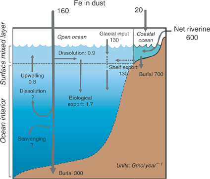
Several box models of iron biogeochemistry with varying complexity have been constructed to better understand and describe iron cycling in the ocean and its relationship to external sources such as the atmosphere and the continents.[ 11 – 14 ] Our intention is not to repeat the conclusions of that work here. Rather we will use a simple Broecker-style 2-box model of the iron cycle in the ocean (Fig. 1) for illustrative purposes. We recognise that for an element of such short residence time, such a simple box model is not very realistic. In particular, no attempt is made to account for chemical speciation in the model. Nonetheless, it attempts to demonstrate that iron biogeochemistry has several distinctive features that are not found with other, less reactive elements of biological importance.
|
First, it is obvious that the iron cycle is dominated by external sources and sinks of iron, mostly in particulate and/or colloidal phases. Input fluxes of iron in dust, glacial inputs and iron-containing riverine colloids and particulates are gigantic in relation to those apparently required by oceanic phytoplankton and to the oceanic inventories of ‘dissolved Fe’. What is quite uncertain, however, is the extent to which these particulate fluxes are harnessed by the ocean’s microbial community.
Rivers transport significant quantities of iron released by the weathering of rocks and soils. However, almost all of this iron is in the form of colloidal ferric hydroxides and oxides, in close association with natural organic matter that stabilises the colloids.[ 15 – 20 ] The conventional paradigm is that these colloids are removed by flocculation in estuaries, although this view is actually based largely on observed transformations of colloidal Fe into filterable particulates. Much less is known, in quantitative terms, about the depositional fate of these particulates in estuaries, shelf waters or cross-shelf transport, particularly in the face of likely episodic flushing of sediments under storm conditions, despite considerable research.[ 21 – 23 ]
In a similar way, continental dust transports globally significant quantities of iron to the ocean, and this is likely to be the main external iron source in remote offshore regions. Just as with riverine iron, however, we know only a little about how much of this iron is biologically utilised. The solubility of iron in dust appears to be low, perhaps less than 1%, but major questions remain concerning the effects of atmospheric cloud recycling on solubility[ 24 – 26 ] and the role of photochemistry and organic ligands on iron dissolution and uptake by microbes.[ 27 ] Recent work suggests that some upper ocean microbes can assimilate colloidal iron directly.[ 28 , 29 ]
The deposition of iron into deep ocean sediments is interesting. The pelagic clay fraction of deep ocean sediments contains very high concentrations of ferro-manganese oxides, together with other trace elements that are presumably associated with these mineral phases through scavenging from solution in the water column.[ 30 ] The concentrations of clay-bound iron are particularly high in the Pacific Ocean, where particle scavenging processes are more intense than in the Atlantic.[ 31 – 35 ] The high enrichment of Fe and Mn in pelagic clays relative to their terrestrial precursors clearly implies that somewhere in the water column, redox transformations of these elements takes place, enriching clay particle surfaces with Fe and Mn, and associated adsorbed elements. Is this transformation mediated by microbes, and at which depth strata in the water column does this predominantly occur? Hydrothermal sources of Fe and Mn may also be important in this context.[ 35 ] But is this a significant iron source for microbes in the euphotic zone?
Iron in seawater
Like most trace elements, the history of understanding iron distributions in the ocean has been fraught with problems of sample contamination and thus reliability of sampling and analytical methods.[ 31 , 36 ] The first major intercalibration exercise organised as an adjunct to the SCOR-IUPAC Working Group 109[ 37 ] revealed significant variations between laboratories in the simple determination of ‘dissolved Fe’[ 38 ] but the more recent SAFE Iron Intercomparison Cruise showed a 10-fold improvement, with systematic differences between most of the analytical methods that appear to be <0.05 × 10⁻⁹ M which is very pleasing.[ 39 ]
Some general properties of oceanic Fe are now revealed. The seminal paper of Johnson et al.[ 40 ] and companion articles[ 41 – 44 ] made the first summary of important trends. Johnson et al. argued that although dissolved iron exhibits vertical concentration profiles that resemble those of macronutrients in general shape, it also has near constant concentrations of ~0.7 × 10⁻⁹ M in deep waters, without any inter-basin fractionation. They ascribe this to stabilisation of iron against removal by scavenging through the agency of ubiquitous iron-binding ligands. Boyle has argued that the dataset used by the authors was somewhat selective, and that data were lacking for those regions likely to be most different.[ 42 ] Indeed, more recent measurements show significantly lower deep water concentrations in the Southern Ocean[ 45 ] and higher ones at depth in the equatorial Atlantic.[ 46 , 47 ]
A considerable body of work, particularly by Kuma and associates, on the solubility of FeIII in seawater points towards the important role of natural organic matter in controlling the solubility of iron in surface and deep waters by forming complexes with FeIII, and the potential generation of ligands from oxidation of organic material in deep waters.[ 48 – 55 ] In addition, several direct measurements of the complexation of FeIII by organic matter in seawater have been reported, mainly as a result of electrochemical titration measurements. These measurement methods and results have been recently reviewed by Bruland and Rue.[ 56 ] Briefly, most techniques involve reacting the sample with a known concentration of a competing iron-binding ligand which forms an electroactive complex that can be detected by electrochemical means, although other detection methods are possible. A series of sample aliquots with increasing amounts of FeIII added to them are measured, and the results of this ‘ligand titration’ can be analysed by various mathematical means to determine the apparent stability constant and total concentration of one or more unknown iron-binding ligands.[ 56 ] An important factor is the so-called ‘detection window’, which is set by the concentration and stability of the competing ligand. Complexes formed by natural ligands that are much weaker than those of the added synthetic ligand cannot be observed.[ 57 ] Therefore results reported by this technique must be viewed carefully in this regard with respect to the number of different ligand classes observed. Table 1 summarises some of the published studies.
|
The common feature of most of these studies is the presence of very strong Fe-binding ‘ligands’ in surface waters which mean that almost all of the FeIII is present in the form of ‘ligand complexes’. In some cases, if an appropriate detection window has been employed (low values of the side reaction coefficient α in Table 1), more than one class of ligand is observed, a so-called strong ligand L1, which predominates in the upper water column and a more abundant, but less strongly complexing ligand L2 deeper in the water column.[ 58 , 59 ] Most authors observe only the strong ligand L1 (Table 1), but these differences seem to be largely a function of the analytical window employed[ 56 , 57 ] or because the concentration of dissolved Fe is so high that the strong L1 has been fully complexed.[ 60 ] In reality, there may be hundreds or even thousands of discrete ligand types in seawater, but it is almost impossible to achieve resolution of more than one or two discrete classes through existing measurement methods.
Nonetheless, the existence of iron binding ligands, whatever they are, seems to be crucial to maintaining the overall inventory of ‘dissolved’ iron in the ocean. Without their presence, scavenging and the limit set by the solubility of ferric hydroxide in seawater[ 61 – 63 ] significantly less iron would be present in deep water. The question is, does this matter? In other words, is the upwelling of deep water important to the surface water iron requirements of phytoplankton, as suggested by Watson and co-authors?[ 64 , 65 ] We will return to this important point later in this paper.
The provenance of ligands
Why is there more than one class of iron-binding ligand? As already mentioned, the classes L1 and L2 are operationally defined, and in reality there are probably a wide range of ligand classes. Nevertheless it is informative to explore where and when (over geological time) these ligand classes evolved. The discovery of Fe-binding ligands gave rise to speculation about their chemical nature and origin.[ 57 , 58 , 66 ] Are iron-binding ligands discrete molecules or complex mixtures? Are they of direct biological origin? The discovery that siderophore-like compounds are produced by various marine microbes in laboratory culture,[ 66 – 70 ] and the similar conditional formation constants of seawater Fe-binding ligands and known siderophores suggested that the seawater ligands do have a direct biological origin and are probably not very large in molecular size (300–1000 Da).[ 71 , 72 ] This provokes the intriguing paradigm of microbes competing for this scarce trace element by sequestering a specific iron-collection ‘agent’. Yet it raises important questions as well.
For a start, it is necessary to invoke iron acquisition mechanisms at the cell surface of the microbe that unlock iron directly from such complexes, because their dissociation kinetics are probably too slow to support growth from the very small fraction of un-complexed iron that maintains equilibrium with the complexed pool of iron. In this regard, mechanisms involving photo-dissociation, ligand exchange and cell surface bound ferri-reductase enzymes have all been advanced.[ 73 – 76 ]
Thus, it seems very likely that iron-binding ligands figure centrally in the acquisition of iron by microbes in the euphotic zone. Equally, it would seem to beggar belief that microbes in the upper ocean would adopt a strategy that populates the whole ocean with such specific iron-binding molecules. The energetic cost of synthesising such molecules would seem to be just too high. Perhaps, as some results suggest,[ 58 , 59 ] iron binding ligands in deep water are recalcitrant/refractory in nature, and might be analogous to the humic material in terrestrial soil and water that is characteristic of organic matter degradation. The specific nature of iron-binding ligands is also difficult to reconcile with the observation that the chemical speciation of many other transition metals is also dominated by organic complexes,[ 77 , 78 ] including Zn,[ 79 – 81 ] Cd,[ 82 ] Cu,[ 83 – 86 ] Ni[ 85 ] and Co.[ 87 ]
As already mentioned, much of this humic material is colloidal in nature in terrestrial environments. This may also be the case in the ocean. Recent studies using ultrafiltration[ 88 ] demonstrate that colloidal ‘ligands’ account for a significant fraction of the ‘dissolved, complexed’ iron in the water column. Fig. 2a compares the results for soluble (<0.02 μm filter pore size) and colloidal (0.02–0.4 μm pore size) iron at several sites in the oligotrophic ocean. Colloidal iron concentrations are highest in surface waters and decrease with depth, consistent with the expected scavenging of colloids by sinking particles. By contrast, soluble Fe concentrations are lowest at the surface and increase with depth in a macronutrient-like manner. In the deep ocean, about half of the dissolved iron is colloidal, with a generally greater fraction in the surface layer. This is the essential paradox presented by iron – it behaves like a micro-nutrient yet has a very short oceanic residence time because of its insolubility and particle reactivity. Obviously more work on the colloidal nature of iron and iron-binding ligands is needed because of the important implications for understanding iron uptake mechanisms in the euphotic zone.
|
When the results in Fig. 2a are considered in the light of measurements of the speciation of iron, it is clear that much of the so-called dissolved iron in seawater that is bound to strong Fe-binding ligands must be in a colloidal state and not in true solution. This does not sit well with the notion that the strong Fe-binding ligands are true siderophores. In support of this, Fig. 2b shows measurements of soluble Fe-binding ligands <0.02 μm particle size made in the same ultrafiltraton study.[ 88 ] This is the fraction that should contain true siderophores. Interestingly, the soluble ligands show very low concentrations in surface waters, much lower than those of the Fe-binding ligands measured by electrochemical techniques. For example, Fig. 2c shows the vertical distribution of strong Fe-binding ligand L1 in the North-eastern Atlantic determined by electrochemical titrations by Boye et al.[ 89 ] This would seem to make it unlikely that L1 can represent siderophore-like compounds, which have relatively low molecular mass (300–1000 Da),[ 72 ] even though the apparent stability complexes of the L1 ligands, and siderophores, are very similar. However, these contradictory observations can be resolved if the siderophores, upon release into seawater by microbes, become strongly associated with organic colloids, as recently suggested by Buck et al.[ 90 ] Again, we will return to this important point later on.
We now speculate a little about iron biogeochemistry based on a distillation of the current knowledge already described. Most scientists working in the field believe that iron speciation in the ocean is dominated by ‘complexing’ with organic matter, although recently even this has been questioned.[ 91 – 95 ] There may be two distinct types of such ‘complexation’. In surface waters, prokaryotic organisms (i.e. those without a cell nucleus, e.g. heterotrophic bacteria and cyanobacteria) may synthesise and release siderophores in an attempt to efficiently sequester iron to meet their metabolic needs. The ability of prokaryotes to make specific iron-binding ligands suggests a biological response to changing iron chemistry in the ancient ocean. Such a response, in the late Archaean and early Proterozoic periods, is consistent with what is referred to by Falkowski and Vargas[ 96 ] as a period of metabolic experimentation and innovation when key biochemical pathways evolved (Fig. 3).

|
Interestingly, eukaryotic plankton (i.e. containing a nucleus), which evolved later that prokaryotes in geological time (the Proterozoic era, Fig. 3), do not seem to produce siderophore-like compounds. Although there have been some reports of siderophore production by eukaryotic phytoplankton such as dinoflagellates in laboratory culture,[ 69 , 70 ] it is probable that these cultures were not axenic (i.e. they were contaminated by heterotrophic bacteria) and thus the siderophores were produced by the heterotrophic bacteria [S. Wilhelm, pers. comm.]. So if eukaryotic phytoplankton do not produce siderophores, how do they access iron, most of which is organically bound?[ 58 ] Either they developed alternative iron acquisition mechanisms as they evolved and diversified (Fig. 3, and see reviews by Quigg et al.[ 97 ] and Finkel et al.[ 98 ]) or were able to obtain iron from other sources.[ 76 ]
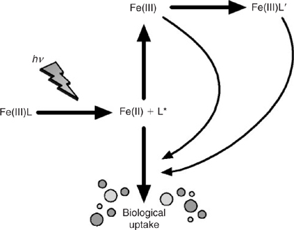
The siderophore-like specific iron-binding ligands are not likely to be long-lived on the time scale of oceanic mixing otherwise we should see much more pronounced penetration of L1 to depth. Moreover, there is increasing evidence that these biologically produced ligands are highly photochemically reactive, which may represent a significant loss process in the upper ocean for siderophores[ 27 ] (Fig. 4). These ligands are at highest concentrations in the mixed layer, and with winter overturn, should be gradually mixed down the water column. This suggests that the task of maintaining iron in solution in the deep ocean falls to less specific molecules and colloids, which we term the ligand soup. This is based on the notion that almost any organic matter, after suitable ‘cooking’, will most likely generate metal-binding ligands. Potential sources of ligand soup include the breakdown of biological material in sinking particles and residual terrestrial organic matter transported from the continental shelves.[ 99 , 100 ] The key point, which we address in more detail below, is that the ligand soup is the inevitable outcome of the development of a food web involving grazers and the formation of biological aggregates such as fecal pellets.[ 101 ] Note that cross shelf transport is also an important source of dissolved and colloidal Fe to the deep ocean[ 102 ] (Fig. 1).
|
Interactions between the ligand soup and FeIII increase the inventory of FeIII in the ocean by several-fold at least, as indicated by the solubility studies mentioned earlier. Although geochemical budgets indicate that upwelled iron is the primary driver for phytoplankton growth in some ocean regions,[ 13 , 103 , 104 ] the biological availability of this iron has not been demonstrated experimentally. Perhaps the role of siderophores is to sequester iron from the ligand soup complexes (see later)?
Whatever the provenance, if we accept the notion of a general ligand soup controlling the overall iron budget of the deep sea, this raises important questions about when in the geological past these molecules might have become pivotal to the iron budget. Although we know nothing about their chemical nature, it seems almost certain that they must be highly refractory in nature, as suggested, for example, by the great age of deep water organic matter.[ 99 ] Some, such as porphyrin structures,[ 76 ] might be closely related to cellular metabolic components (e.g. breakdown products of chlorophyll), but others might be the result of condensation and oxidation reactions of cells similar to those observed in terrestrial environments.[ 99 ] This would seem to argue in favour of materials characteristic of the modern, oxygenated ocean. Therefore, we shall conclude this review by summarising the current state of knowledge about the evolution of iron biogeochemistry over geological time, speculating still further about its implications for the modern ocean.
Evolution of the iron and oxygen chemistry of the ocean
There has been considerable recent progress in unraveling the secrets of the early ocean,[ 105 ] particularly through the use of a variety of isotopic tracers[ 106 ] and the growing application of the findings from genome sequencing to understanding ocean paleobiology.[ 96 ] From this emerges a sequence of events in which iron has been intimately involved (Fig. 3).
The Archaean and early Proterozoic ocean (Fig. 3; >1850 million years BP) were characterised by anoxic conditions but low in dissolved sulfide. At this time, dissolved iron in the ocean was at its highest, primarily as dissolved FeII. The first forms of life, including the heterotrophic bacteria evolved early on in this scenario, perhaps as early as 3200 million years ago, but certainly by 2700 million years ago.[ 96 ] Oxygen-generating photosynthetic cyanobacteria are thought to have bloomed periodically during this phase, with most of the O2 they generated ending up in the vast iron deposits known as banded iron formations (BIF). These are thought[ 107 ] to form through seasonal blooms of planktonic organisms that oxygenate surface waters (and deplete them of iron), after which overturn of deep waters gives rise to mixing of FeII-rich subsurface waters with surface water O2, which results in precipitation of iron oxides. The fact that BIFs are made up of mixed oxidation state iron oxides containing FeII, such as Fe3O4, suggests that the deep water remained anoxic (i.e. FeII-rich) throughout this period. This is also supported by sulfur isotope measurements that indicate very little dissolved sulfate in the ocean at this time.[ 106 ]
It is, therefore, not surprising that cyanobacterial enzyme systems using iron evolved during this early period (Fig. 3). FeII was abundant in seawater, perhaps as much as 100 × 10–6 M,[ 10 ] and the FeII–FeIII redox couple provides for facile electron transfer reactions. This does not rule out a role for FeIII however. Small concentrations of O2 were likely generated by the photolysis of H2O in the atmosphere. In addition, the early evolution of water-splitting cyanobacteria would have generated O2 in the surface ocean, at least as a trace component in the Archaean period, which readily oxidises FeII as evidenced by, for example, the BIF deposits. Because FeIII is so insoluble, the maintenance of an FeII-dominant ocean would have depended on almost complete consumption of O2 in surface waters, or by loss to the atmosphere. Organic matter oxidation in surface waters would have likely played a role here. Finally, recent measurements of Fe isotopes in BIF deposits provide support for this evolution of the chemistries of Fe, O2 and S.[ 108 , 109 ]
It is important to note that organic matter recycling was likely to be very different during this period.[ 101 ] Little organic matter is found in formations like the BIFs. In the modern ocean, most of the organic matter flux to deep waters is mediated by rapidly settling biogenic material such as zooplankton fecal pellets.[ 101 ] These did not evolve until the surface ocean became oxic and the oceanic biota diverged into eukaryotes and then animals such as zooplankton.
In the second phase of ocean evolution, beginning ~1800 million years ago, O2 production had increased enough that rising atmospheric O2 concentrations began to oxidise surface rocks to a considerable extent (Fig. 3). Thus the Earth became the ‘rusty planet’. At this time, banded iron formations disappear from the geological record and are replaced by more oxidised red iron oxides. While the surface ocean was now probably oxic most of the time, a key feature of the ocean in this part of the Proterozoic period is the dominance of bacterial sulfate reduction in the deep ocean. This arose because increased oxidation of terrestrial pyrites began delivering significant quantities of sulfate to the ocean. While the loss of Fe through the prior BIF formation might have threatened to deplete the oceanic inventory of the element that had become vital for biological systems, the advent of reduced sulfur species, specifically HS–, in the deep ocean overcame this potential dilemma by complexing with Fe, maintaining soluble iron levels around 1 × 10⁻⁶ M.[ 10 ]
However, the progressive oxygenation of the surface ocean would have posed problems for the heterotrophic bacteria and cyanobacteria. Both needed to develop the ability to function in the presence of O2, a waste product, in order to survive the transition to the euxinic ocean. One strategy that was important here was the adoption of respiration, an extremely efficient mechanism for obtaining chemical energy. However, the almost complete oxygenation of the surface layer posed a new problem, because FeII became unstable at the expense of the highly insoluble form FeIII. Saito et al.[ 10 ] proposed that these microbes adapted by developing the ability to synthesise siderophores, and we agree with this idea. However, they went on to argue that ‘these organic ligands serve to mimic the aqueous chemistry of the strong metal-sulfide complexes’, and on this point we disagree. While an organic ligand would become necessary to support the iron inventory when the deep ocean becomes fully oxygenated (see later), these conditions did not appear until the close of the Proterozoic. Therefore, we believe the main purpose of the siderophores was to overcome the FeIII solubility problem in oxygenated surface waters of the Proterozoic.
Later in the Proterozoic (Fig. 3), life began its first great blossoming with the development of eukaryotic cells that eventually gave rise to more complex multicellular organisms. In addition, the development of an ozone layer allowed life forms to migrate onto the land for the first time, from which even greater diversity resulted. As far as ocean biogeochemistry is concerned, a key issue at this time would have been the starting up of the great fecal pellet biological pump, which presumably gave rise to enhanced organic matter transport into the deep ocean and the potential for the development of organic matter breakdown products – i.e. the ligand soup. Not much later, the eukaryotic explosion gave rise to the blossoming of terrestrial plants, which itself switched on the formation of terrestrial organic matter transported into the coastal ocean, and perhaps further.[ 99 , 100 ]
At the close of the Proterozoic period, the ocean evolved into its present state, characterised by oxic conditions throughout the deep ocean. We propose that the development of the ligand soup assisted in maintaining FeIII levels in the deep ocean to values higher than would be expected on the basis of FeIII solubility alone[ 62 ] by replacing the sulfide ion as the predominant solubilising ligand for FeII with one that complexed the now predominant FeIII. However, it appears that the ligand soup and/or prokaryotic siderophores are a poor substitute for HS– of the Proterozoic period, and dissolved Fe levels thus fell to around 1 × 10⁻⁹ M characteristic of the present day.
Several new strategies were needed by the eukaryotes who appear to lack the ability to synthesise siderophores.[ 110 ] Thus enzyme substitutes not containing iron evolved, e.g. the substitution of flavodoxin for ferredoxin.[ 111 ] Iron-containing enzyme systems became much more efficient in terms of their iron use, especially for microbes adapted to the remote ocean.[ 112 ] Another interesting twist in this story of biochemical adaption is the adoption of molybdenum as a co-factor in several iron-containing enzymes. Indeed, Fe and Mo are uniquely related in that in the modern ocean, Fe has become an element present in seawater in only trace amounts but is perhaps one of the most abundant transition elements in organisms, whereas Mo is the opposite. Mo, in the form of the highly unreactive molybdate ion, MoO4 2–, is conservative in seawater with an oceanic concentration of ~100 × 10–9 M. However, in the Archaean Ocean, Mo was just simply not abundant enough to figure prominently in early enzyme biochemistry.
An interesting related factor is the effect of these changes in ocean chemistry on the availability of other transition metals of biological importance. The most marked change is that for Cu2+, an ion that is extremely insoluble in the presence of dissolved sulfide. Oxygenation of the deep sea gave rise to increases in available Cu2+ of ~16–17 orders of magnitude. Since Cu2+ is extremely good at blocking the coordination centres of many metallo-enzymes, this would have constituted another great trace metal crisis for oceanic biota. So much so that the ubiquitous Cu2+-binding organic ligands observed in the modern ocean are thought to be a specific Cu2+-detoxification mechanism.[ 113 , 114 ]
This raises another important issue. As already mentioned, the presence of strong binding ligands for transition metal ions in the ocean is almost ubiquitous, which might suggest that the ligand soup is responsible for this property. Indeed, in the field of coordination chemistry, it is relatively simple to construct an organic ligand that will bind strongly to a whole range of transition metal ions – simple iminodiacetates such as EDTA (ethylenediamine tetraacetate) are a good example. However, it is much more difficult to design a ligand that binds a particular metal ion strongly to the exclusion of others having similar coordination chemistry. The latter is generally the domain of highly specific biological macromolecules. We suggest that competitive ligand-binding experiments should be done to test the selectivity of seawater ligands. Such experiments must be carefully designed to ensure that there is not a large excess concentration of the ligand present, which will mask any competitive binding effects.
Another interesting feature is the significant increases in availability of Cd2+ and Zn2+ in the modern ocean, again largely because of sulfide insolubility. Metalloenzymes using these metals did not evolve until the advent of the eukaryotes when the ocean was fully oxygenated:[ 10 ] they were simply not abundant enough before that.
The impact of ligands on iron biogeochemistry
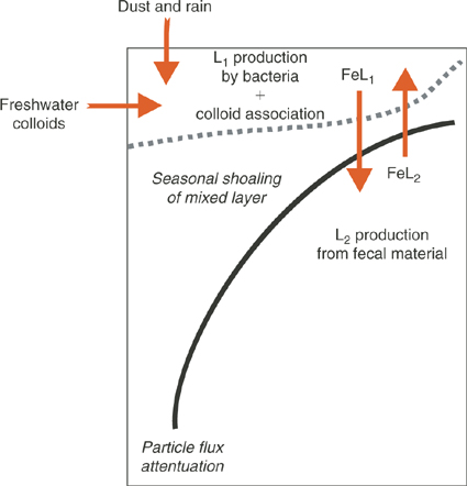
Fig. 5 shows schematically how iron-binding ligands might impact on iron biogeochemistry in the ocean. While undoubtedly there are many classes of Fe-binding ligands present in seawater, we have chosen to simplify this to two different classes: a strong L1 ligand generated in surface waters by microbial activity and the less specific and weaker binding ligand L2 that comprises the ligand soup. This distinction is at least suggested by some of the speciation studies, even though the problems of different detection windows do not allow us to be more definitive. In any case, our classification is designed to be a conceptual aid to guide new research initiatives.
|
If, as we conjecture, L1 ligands are generated by the activity of marine microbes, then they will have the highest concentrations in the mixed layer where heterotrophic and cyanobacterial activity and abundances are highest, and will only undergo transport into the underlying waters by vertical water exchange such as advection, diffusion and downwelling. These processes will vary seasonally as the mixed layer shoals and deepens. As mentioned earlier, these L1, siderophore-like ligands most likely become rapidly associated with colloidal organic matter.[ 90 ] Such an association is required to reconcile their low molecular weights, and high conditional stability constants with the apparently colloidal nature of electrochemically determined strong ligands.
By contrast L2 ligands, we postulate, are primarily associated with particle decomposition, and therefore should have highest concentrations in the subsurface ocean because sinking particles will decay according to the ‘Martin curve’, a power law function.[ 115 ] In a similar way, Fe bound by L2 will be transported into the mixed layer through upwelling and vertical advection and diffusion.
This raises the important question about the role of Fe bound by L2 from deep water. It has been argued that upwelling is the main source of Fe for phytoplankton in the mixed layer of the Southern Ocean.[ 65 ] However, we know very little about the bioavailability of Fe bound to L2 other than information gained from the measurement of stability constants. Does Fe brought to the surface mixed layer bound to L2 interact with the stronger ligands L1, undergoing ligand exchange? This is likely, since generally there is sufficient excess L1 in surface waters to bind all of the dissolved Fe. Is this transformation a key part of the strategy for the pelagic biota gaining access to Fe? One way to resolve this would be to experimentally investigate the effect of deep water Fe on phytoplankton laboratory cultures to determine whether or not they can access Fe bound by the weaker L2 ligands. A second useful experiment would be to mix surface and deep waters together, and use electrochemical methods to determine if the equilibrated mixture assumes the properties expected of each end member.
Similar questions need to be asked about the role of ligands in freshwater Fe colloids that enter shelf regions, and ligands in rain during the wet deposition of atmospheric dust. Is Fe in surface water in equilibrium with the various ligands entering from all of these sources? Does L1 dominate? How is this affecting different algal classes, some of which can access Fe bound by L2 [ 76 ]?
The dynamic aspects of the ligand cycle depicted in Fig. 5 are equally important. For example, there is evidence from several mesoscale iron enrichment studies that iron supply can either directly or indirectly result in increased concentrations of iron-binding L1 ligands.[ 27 ] If L2 is derived from sinking particles, will its concentration scale to the magnitude of particle decomposition which varies regionally and with depth? What is the residence time of these L2 class? Can any useful parallels be drawn with other components of the sinking particle flux, e.g. nutrients or carbon? Will L2 set an upper value on the concentration of Fe in deep water?
Similarly in the mixed layer, if excess Fe is supplied from external sources will the L1 ligand become saturated, or will microbes produce more siderophores?[ 116 ] Are microbes ‘monitoring’ the concentration of dissolved Fe?
Recent modelling studies have begun to explore how ligands will impact on, and set constraints on, the biogeochemistry of iron in the global ocean.[ 11 , 12 , 117 ] To further guide the development of these models, we need to have more detailed answers to the questions raised above.
Key natural laboratories to test the interactions of different ligand classes with respect to iron cycling are estuaries, the interface between the surface and subsurface ocean and dust deposition (wet and dry) into the surface ocean.
Key methodological developments include isolation of Fe bound by ligands in sufficient quantities to apply chemical techniques for structure determination, extending the work of Macrellis et al.[ 72 ] and also help to understand how ligand production by microbes is induced and controlled. This will also help to make (or break) the conceptual link between L1 and siderophores. New analytical techniques (other than electrochemical, or in conjunction with electrochemistry) to better constrain measured ligand classes are also desirable. In particular, identifying marine v. terrestrial components of the ligand classes is very important. Studies should also be made of the Fe-binding properties of refractory iron-containing freshwater organic matter colloids. Finally, using unpreserved samples from sediment traps as a source of sinking particles to examine the production of L2 from decomposing particulates (time scale of days) should be a fruitful area of future study.
We fully recognise that this review has raised more questions than it has answered. Nonetheless, this appears to be the nature of iron biogeochemistry. The more we discover, the more we realise that we don’t understand. It is our hope that the ideas and speculations presented here, whether they turn out to be right or wrong, will nevertheless stimulate further useful research in this fascinating area of science.
Conclusions
-
The evolution of first prokaryotes, followed by eukaryotes, appears to be the main determinant behind the development of the two ligand class system. The strong L1 ligand is likely to be a siderophore produced only by prokaryotes in response to the progressive oxygenation of the surface waters commencing in the early Proterozoic era. The weaker L2 ligand is a byproduct of the degradation of sinking biological particles that did not appear until complete oxygenation of the deep ocean which marked the end of the Proterozoic, and was initiated by the evolution of complex food webs.
-
The only real evidence that strong L1 ligands are siderophores is that their conditional stability constants for Fe-binding are similar. However, this is difficult to reconcile with recent observations on the vertical distributions of iron and iron-binding ligands in different size fractions. Most of the dissolved Fe, and most of the Fe-binding ligands, appear to be colloidal, yet siderophores are relatively small molecules. These disparate observations indicate that bacterial siderophores, if they are responsible for most of the strong Fe-binding, must be modified after production to become associated with colloidal materials.
-
We currently know very little about the specificity of Fe-binding ligands. Siderophores (L1) are likely to be highly specific for FeIII, whereas the ligand soup (L2) that we propose is likely to bind metal ions more generally. The latter type of ligand is consistent with the observation that the chemical speciation of many other transition metals is also dominated by organic ligands.
-
Although the production of ligands in response to altered environmental conditions such as Fe enrichment has been observed, the underlying mechanisms behind these changes remain unclear.
Acknowledgements
The authors are grateful to the University of Otago, the National Institute of Water and Atmospheric Research for support, and to the Marsden Fund of the Royal Society of New Zealand and the Foundation for Research, Science and Technology for financial support. We also thank our many scientific colleagues and post-graduate students for their contributions to our work, and the reviewers of this paper for useful input. We are grateful to Steve Wilhelm for his personal communication concerning bacterial contamination of laboratory algal cultures.
[1]
J. H. Martin ,
R. M. Gordon ,
S. E. Fitzwater ,
Iron in Antarctic waters.
Nature 1990
, 345, 156.
| Crossref | GoogleScholarGoogle Scholar |
[Verified 4 March 2004].
[97]
A. Quigg ,
Z. Finkel ,
A. Irwin ,
Y. Rosenthal ,
Y.-H. Ho ,
J. Reinfelder ,
O. Schofield ,
F. Morel ,
et al. The evolutionary inheritance of elemental stoichiometry in marine phytoplankton.
Nature 2003
, 425, 291.
| Crossref | GoogleScholarGoogle Scholar | PubMed |

[98]
Z. V. Finkel ,
A. Quigg ,
J. A. Raven ,
J. R. Reinfelder ,
O. E. Schofield ,
P. G. Falkowski ,
Irradiance and the elemental stoichiometry of marine phytoplankton.
Limnol. Oceanogr. 2006
, 51, 2690.
[99]
J. E. Bauer ,
E. R. M. Druffel ,
D. M. Wolgast ,
S. Griffin ,
Temporal and regional variability in sources and cycling of DOC and POC in the northwest Atlantic continental shelf and slope.
Deep-Sea Res. Pt. II 2002
, 49, 4387.
| Crossref | GoogleScholarGoogle Scholar |
[100]
J. Hwang ,
E. R. M. Druffel ,
S. Griffin ,
K. L. Smith ,
R. J. Baldwin ,
J. E. Bauer ,
Temporal variability of Δ14C, δ13C, and C/N in sinking particulate organic matter at a deep time series station in the northeast Pacific Ocean.
Global Biogeochem. Cy. 2004
, 18, GB4015.
| Crossref | GoogleScholarGoogle Scholar |
[101]
C. Bjerrum ,
D. E. Canfield ,
T. Kiørboe ,
G. A. Jackson ,
From dissolved organic carbon to marine snow in the prokaryote dominated Precambrian oceans.
Geochim. Cosmochim. Acta 2004
, 68, A787.
[102]
R. Raiswell ,
M. Tranter ,
L. G. Benning ,
M. Siegert ,
R. De’ath ,
P. Huybrechts ,
T. Payne ,
Contributions from glacially derived sediment to the global iron (oxyhydr)oxide cycle: implications for iron delivery to the oceans.
Geochim. Cosmochim. Acta 2006
, 70, 2765.
| Crossref | GoogleScholarGoogle Scholar |
[103]
S. Blain ,
B. Queguiner ,
L. Armand ,
S. Belviso ,
B. Bombled ,
L. Bopp ,
A. Bowie ,
C. Brunet ,
et al. Effect of natural iron fertilization on carbon sequestration in the Southern Ocean.
Nature 2007
, 446, 1070.
| Crossref | GoogleScholarGoogle Scholar | PubMed |
[104]
P. W. Boyd ,
Biogeochemistry: iron findings.
Nature 2007
, 446, 989.
| Crossref | GoogleScholarGoogle Scholar | PubMed |
[105]
D. C. Catling ,
M. W. Claire ,
How Earth's atmosphere evolved to an oxic state: a status report.
Earth Planet. Sci. Lett. 2005
, 237, 1.
| Crossref | GoogleScholarGoogle Scholar |
[106]
A. Anbar ,
A. Knoll ,
Proterozoic ocean chemistry and evolution: a bioinorganic bridge?
Science 2002
, 297, 1137.
| Crossref | GoogleScholarGoogle Scholar | PubMed |
[107]
A. Kappler ,
C. Pasquero ,
K. O. Konhauser ,
D. K. Newman ,
Deposition of banded iron formations by anoxygenic phototrophic Fe(II)-oxidizing bacteria.
Geology 2005
, 33, 865.
| Crossref | GoogleScholarGoogle Scholar |
[108]
N. Dauphas ,
M. van Zuilen ,
M. Wadhwa ,
A. M. Davis ,
B. Marty ,
P. E. Janney ,
Clues from Fe isotope variations on the origin of early Archean BIFs from Greenland.
Science 2004
, 306, 2077.
| Crossref | GoogleScholarGoogle Scholar | PubMed |
[109]
L. Kump ,
OCEAN SCIENCE: ironing out biosphere oxidation.
Science 2005
, 307, 1058.
| Crossref | GoogleScholarGoogle Scholar | PubMed |
[110]
A. Butler ,
Acquisition and utilization of transition metal ions by marine organisms.
Science 1998
, 281, 207.
| Crossref | GoogleScholarGoogle Scholar | PubMed |
[111]
J. La Roche ,
P. W. Boyd ,
R. M. L. McKay ,
R. J. Geider ,
Flavodoxin as an in situ marker for iron stress in phytoplankton.
Nature 1996
, 382, 802.
| Crossref | GoogleScholarGoogle Scholar |
[112]
R. F. Strzepek ,
P. J. Harrison ,
Photosynthetic architecture differs in coastal and oceanic diatoms.
Nature 2004
, 431, 689.
| Crossref | GoogleScholarGoogle Scholar | PubMed |
[113]
J. W. Moffett ,
L. Brand ,
Production of strong, extracellular Cu chelators by marine cyanobacteria in response to Cu stress.
Limnol. Oceanogr. 1996
, 41, 388.
[114]
J. W. Moffett ,
Temporal and spatial variability of copper complexation by strong chelators in the Sargasso Sea.
Deep-Sea Res. 1995
, 42, 1273.
| Crossref | GoogleScholarGoogle Scholar |
[115]
J. H. Martin ,
G. A. Knauer ,
D. M. Karl ,
W. W. Broenkow ,
VERTEX: carbon cycling in the northeast Pacific.
Deep-Sea Res. Pt. II 1987
, 34, 267.
| Crossref | GoogleScholarGoogle Scholar |
[116]
P. L. Croot ,
A. R. Bowie ,
R. D. Frew ,
M. T. Maldonado ,
J. A. Hall ,
K. A. Safi ,
J. La Roche ,
P. W. Boyd ,
C. S. Law ,
Retention of dissolved iron and Fe(II) in an iron induced Southern Ocean phytoplankton bloom.
Geophys. Res. Lett. 2001
, 28, 3425.
| Crossref | GoogleScholarGoogle Scholar |
[117]
K. Fennel ,
M. R. Abbott ,
Y. H. Spitz ,
J. G. Richman ,
D. M. Nelson ,
Impacts of iron control on phytoplankton production in the modern and glacial Southern Ocean.
Deep-Sea Res. Pt. II 2003
, 50, 833.
| Crossref | GoogleScholarGoogle Scholar |
[118]
[119]
[120]
W. G. Sunda ,
S. Huntsman ,
Iron uptake and growth limitation in oceanic and coastal phytoplankton.
Mar. Chem. 1995
, 50, 189.
| Crossref | GoogleScholarGoogle Scholar |
[121]
E. Rue ,
K. Bruland ,
The role of organic complexation on ambient iron chemistry in the equatorial Pacific Ocean and the response of a mesoscale iron addition experiment.
Limnol. Oceanogr. 1997
, 42, 901.
[122]
[123]
J. T. Cullen ,
B. A. Bergquist ,
J. W. Moffett ,
Thermodynamic characterization of the partitioning of iron between soluble and colloidal species in the Atlantic Ocean.
Mar. Chem. 2006
, 98, 295.
| Crossref | GoogleScholarGoogle Scholar |
[124]
M. Gledhill ,
C. M. G. van den Berg ,
Determination of complexation of iron(iii) with natural organic complexing ligands in seawater using cathodic stripping voltammetry.
Mar. Chem. 1994
, 47, 41.
| Crossref | GoogleScholarGoogle Scholar |
[125]
R. F. Nolting ,
L. J. A. Gerringa ,
M. J. W. Swagerman ,
K. R. Timmermans ,
H. J. W. de Baar ,
Fe(III) speciation in the high nutrient, low chlorophyll Pacific region of the Southern Ocean.
Mar. Chem. 1998
, 62, 335.
| Crossref | GoogleScholarGoogle Scholar |
[126]
F. Tian ,
R. D. Frew ,
S. G. Sander ,
K. A. Hunter ,
M. J. Ellwood ,
Organic Fe(iii) speciation in surface transects across a frontal zone: The Chatham Rise, New Zealand.
Mar. Freshwater Res. 2006
, 57, 533.
| Crossref | GoogleScholarGoogle Scholar |
[127]
M. Boye ,
A. Aldrich ,
C. van den Berga ,
J. de Jong ,
M. Veldhuis ,
H. de Baar ,
Horizontal gradient of the chemical speciation of iron in surface waters of the northeast Atlantic Ocean.
Mar. Chem. 2003
, 80, 129.
| Crossref | GoogleScholarGoogle Scholar |
[128]
M. Boye ,
J. Nishioka ,
P. L. Croot ,
P. Laan ,
K. R. Timmermans ,
H. J. W. de Baar ,
Major deviations of iron complexation during 22 days of a mesoscale iron enrichment in the open Southern Ocean.
Mar. Chem. 2005
, 96, 257.
| Crossref | GoogleScholarGoogle Scholar |
[129]
P. L. Croot ,
K. Andersson ,
M. Ozturk ,
D. R. Turner ,
The distribution and speciation of iron along 6°E in the Southern Ocean.
Deep-Sea Res. II 2004
, 51, 2857.
| Crossref | GoogleScholarGoogle Scholar |
[130]
P. L. Croot ,
M. Johansson ,
Determination of iron speciation by cathodic stripping voltammetry in seawater using the competing ligand 2-(2-Thiazolylazo)-p-cresol (TAC).
Electroanal. 2000
, 12, 565.
| Crossref | GoogleScholarGoogle Scholar |
[131]
A. E. Witter ,
G. W. Luther ,
Variation in Fe-organic complexation with depth in the northwestern Atlantic Ocean as determined using a kinetic approach.
Mar. Chem. 1998
, 62, 241.
| Crossref | GoogleScholarGoogle Scholar |
[132]
A. E. Witter ,
D. A. Hutchins ,
A. Butler ,
G. W. Luther ,
Determination of conditional stability constants and kinetic constants for strong model Fe-binding ligands in seawater.
Mar. Chem. 2000
, 69, 1.
| Crossref | GoogleScholarGoogle Scholar |
[133]
A. E. Witter ,
B. L. Lewis ,
G. W. Luther ,
Iron speciation in the Arabian Sea.
Deep-Sea Res. Pt. II 2000
, 47, 1517.
| Crossref | GoogleScholarGoogle Scholar |
[134]
R. T. Powell ,
J. R. Donat ,
Organic complexation and speciation of iron in the south and equatorial Atlantic.
Deep-Sea Res. II 2001
, 48, 2877.
| Crossref | GoogleScholarGoogle Scholar |
[135]
R. T. Powell ,
A. Wilson-Finelli ,
Importance of organic Fe complexing ligands in the Mississippi River plume.
Estuar. Coast. Shelf Sci. 2003
, 58, 757.
| Crossref | GoogleScholarGoogle Scholar |
[136]
R. T. Powell ,
A. Wilson-Finelli ,
Photochemical degradation of organic iron complexing ligands in seawater.
Aquat. Sci. 2003
, 65, 367.