
Population dynamics of chital deer (Axis axis) in northern Queensland: effects of drought and culling
Anthony Pople A * , Matt Amos A and Michael Brennan A
A Queensland Department of Agriculture and Fisheries, 41 Boggo Road, Dutton Park, Qld 4102, Australia.
Wildlife Research 50(9) 728-745 https://doi.org/10.1071/WR22130
Submitted: 15 July 2022 Accepted: 25 May 2023 Published: 15 June 2023
© 2023 The Author(s) (or their employer(s)). Published by CSIRO Publishing. This is an open access article distributed under the Creative Commons Attribution-NonCommercial-NoDerivatives 4.0 International License (CC BY-NC-ND)
Abstract
Context: Chital deer (Axis axis) are long established in the northern Queensland dry tropics, and at high densities are considered pests by cattle graziers. Cost-effective management is difficult for widespread, fluctuating populations of vertebrate pests such as these deer. Historically, control of chital deer has been limited to recreational and some commercial ground-shooting and trapping. Concerns over chital deer impacts were heightened during drought in 2015 and funding became available for aerial culling.
Aim: This study set out to determine (1) distribution and abundance, (2) seasonal reproductive output, (3) potential and actual rates of increase and their determinants, and (4) efficient management strategies for chital deer in the northern Queensland dry tropics.
Methods: In 2014, ~13 000 km2 of the main distribution was surveyed by helicopter. Multiple vehicle ground surveys per year monitored chital deer density on two properties during 2013–2022. Seasonal shot samples of deer on both properties assessed reproductive output during 2014–2016. Aerial surveys during 2016–2020 determined chital deer densities on seven properties, prior to aerial culling on four properties. Finally, the maximum rate of increase of chital deer was calculated from life-history data.
Key results: Regionally, chital deer are patchily distributed and so are best monitored locally where densities can be >50 deer km−2. Vehicle ground surveys recorded an ~80% decline in chital deer populations on two properties over 7–10 months during drought in early 2015, with a similar rate being recorded by aerial survey at a third site. There was little recruitment during the drought, but the decline was seemingly driven by adult mortality. Aerial shooting further reduced populations by 39–88% to <3 deer km−2 on four properties. Where there was no continuing control, culled populations recovered to pre-cull densities or higher after 2.4 years. One unculled property recovered to its pre-drought density after 6 years. Rates of recovery were at or higher than the maximum annual rate of increase for chital deer estimated here as 26–41%.
Conclusions: Drought has a lasting effect on this chital deer population, because of the resulting large population decline and the modest rate of any recovery in the absence of culling. Culling can reduce populations to low density, but the removal rate needs to be sustained to suppress future growth.
Implications: Drought provides a strategic opportunity to further reduce chital deer populations for enduring control. Large reductions are feasible given the clumped dispersion of populations within properties and in the region.
Keywords: aerial shooting, aerial survey, axis deer, numerical response, pest management, population dispersion, rainfall, rate of increase, reproduction, strategic control, ungulate.
Introduction
Fluctuations in the abundance of invasive ungulates and other pest herbivores have important implications for their management, particularly the need for control and its optimal timing (Hone 2007). These fluctuations are pronounced in arid and semi-arid environments, but are also characteristic of cold ‘deserts’ (Caughley and Gunn 1993). In the rangelands of Australia, as populations reach high densities, there is greater concern from landholders over the agricultural and environmental impact of vertebrate pests. During drought, competition for scarce resources similarly leads to calls for control of introduced herbivores (e.g. Dobbie et al. 1993; Williams et al. 1995; Pople et al. 1998; Davis et al. in press). Control effectiveness will depend on the percentage of the population removed but also on whether the population is increasing or decreasing (Pople and McLeod 2000; Pople 2008). It is cost effective to cull animals immediately following drought from an increasing population with abundant resources, when culling mortality will be mostly additional to natural mortality. Animals culled prior to or during a drought may well have died anyway or have freed up resources for others to survive and so culling will be compensated to some extent by reduced natural mortality (Anderson and Burnham 1976; Bartmann et al. 1992; Sinclair and Pech 1996).
In semi-arid and arid Australia, aerial surveys have described fluctuations in populations of feral pigs (Sus scrofa; Gentle et al. 2019), feral goats (Capra hircus; Pople and Froese 2012) and kangaroos (Macropus spp. and Osphranter rufus; McLeod et al. 2021). In semi-arid and arid environments, food supply is driven by highly variable rainfall (Noy-Meir 1973; Stafford Smith and Morton 1990) and drought is a key feature of these cyclical dynamics causing populations to decline markedly and, for species such as kangaroos, take many years to recover (Caughley 1987). This pattern is the result of the convex numerical response of herbivores to food supply (Davis et al. 2002) where there is an upper physiological limit to the modest rate of increase of large herbivores but no limit to their rate of decline in drought.
Four chital deer (Axis axis; two adult males and two adult females) were introduced from Sri Lanka to the property Maryvale in northern Queensland (~100 km north of Charters Towers) in the late 1880s (Roff 1960). The population’s spread from the point of release and increase in abundance appear to have been slow relative to other range expansions in vertebrates (Caughley 1977) on the basis of reports in the 1950s from another property only 50 km away (Roff 1960) and they had yet to reach Charters Towers after 100 years (i.e. <1 km per year) on the basis of anecdotal landholder reports (Forsyth et al. 2019; A. Blokland, pers. comm.). By the 2000s, the population north of Charters Towers was believed to be in the thousands, with increases following above-average rainfall and limited recreational and commercial removals and heavy declines in drought (Jesser 2005). Twinning has been reported (Bentley 1995; Jesser 2005), suggesting a relatively high maximum rate of increase, but such fecundity is not supported by overseas data where twins are rare (e.g. Graf and Nichols 1966; Schaller 1967; Ernest 2003). Nevertheless, chital deer populations have been recorded increasing rapidly following their introduction to a new environment, or the removal of one or more limiting factors where they are established (Duckworth et al. 2015). Hone et al. (2010) calculated a maximum exponential rate of increase for chital deer of rm = 0.79 on the basis of a relationship between rm and age at first reproduction for the Artiodactyla. This equates to more than doubling annually, but the 95% credible intervals for rm were broad (0.21–2).
This study began in 2013 when chital deer were viewed by many landholders as a serious pest animal north of Charters Towers, mainly through competition with cattle for food. The concern about deer in the region provided several study objectives that were to determine the following:
Distribution and abundance of chital deer across their likely range in the region
Body condition and reproductive output of deer across seasons and among areas to determine when and where deer are resource-limited
Potential and actual rates of increase of chital deer in the region and their determinants
Efficient management strategies for deer across the region
Aspects of these objectives have been reported elsewhere (Forsyth et al. 2019; Watter et al. 2019a; Kelly 2021; Bengsen et al. 2022). This paper reports further on each objective, with complementary data, and provides a synthesis.
Materials and methods
The study comprised the following five components: (1) a broad-scale aerial survey was flown across the region to determine chital deer distribution and abundance; (2) two properties were intensively monitored by vehicle ground surveys to monitor changes in chital deer abundance over a longer period; (3) property-based aerial surveys were flown prior to culling events to determine culling effectiveness and the subsequent recovery of the deer population; (4) samples of deer were shot on the two intensively monitored properties to determine seasonal variation in body condition and fecundity; and (5) an estimate of rm was determined from schedules of survival and reproduction.
These components are summarised in Table 1. Details are provided below. As indicated for most of the analyses below, candidate models were compared using Akaike’s information criterion corrected for small sample size (AICc; Burnham and Anderson 1998). Candidate model statistics are shown in Supplementary material Tables S1, S2, S4–S7. Following Burnham and Anderson (1998), models with strong support have AICc differences (ΔAICc) of ≤2.
| Purpose | Location (region or properties) | Method |
|---|---|---|
Broad-scale distribution and abundance of chital deer in 2014 | Region (~13 000 km2) | Helicopter survey |
Change in deer abundance during 2014–2022 in response to rainfall, pasture biomass and culling | Spyglass (property not culled) Niall (culled property) | Vehicle ground surveys with spotlight Numerical response to rainfall and total standing dry matter |
Effectiveness of culling 2016–2018 and recovery to 2021 | Not culled Spyglass, Toomba, Lowholm, Maryvale Creek Culled Niall, Maryvale, Gainsford, Felspar | Helicopter survey Vehicle ground survey (Spyglass and Niall) Aerial and ground-based culling |
Seasonal variation in reproductive output | Niall and Spyglass 2014–2016 Culled properties 2016–2018 | Samples of animals shot solely for research Samples of animals culled from the air Reproductive success related to rainfall and pasture biomass |
Maximum rate of increase Adult sex ratio and age structure | Culled properties 2016–2018 | Euler–Lotka equation Samples of culled animals |
Study area
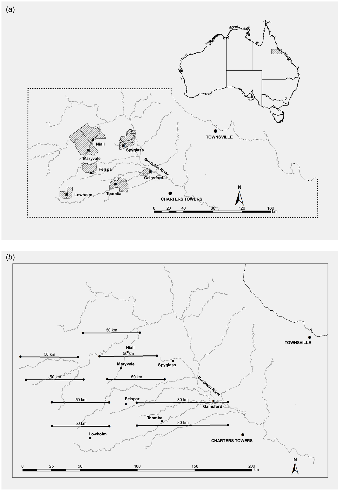
The study was undertaken in the Einasleigh Uplands Bioregion of the dry tropics of northern Queensland (Fig. 1). The region is dominated by open woodlands, with areas of native and introduced grasslands and tall Acacia spp. or Melaleuca spp. shrublands (Forsyth et al. 2019; Watter et al. 2019a, 2020). Land use is predominantly cattle grazing at an average density of 10 animals km−2 (McIvor 2012). Dams and troughs provide water for cattle throughout the region. There are also numerous springs providing permanent water along some creeks and there are wetlands on two of the study properties, namely Toomba and Lowholm (Fig. 1a). Dingoes (Canis familiaris) consume chital deer in the region and are present throughout (Forsyth et al. 2019), despite being controlled by landholders mainly through 1080-poison baiting.
(a) The seven main properties of the study are shown as hatched polygons. (b) The study area was encompassed by nine aerial-survey transect lines that were flown in July 2014. Homesteads of the seven properties where chital deer abundance was monitored in the study are indicated by solid squares. Major tributaries are also shown in grey.
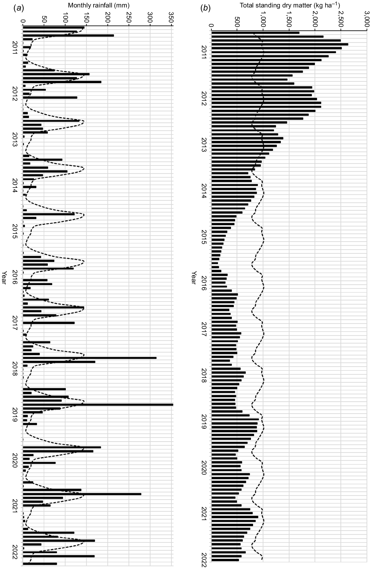
Summers are hot and humid, whereas winters are mild. The climate is strongly seasonal with an extended dry season over winter and early spring. The main limiting factor for grazing animals in the region is poor-quality food during the dry season (April–October) (Mott and Tothill 1984). Average annual rainfall on Spyglass during 1889–2021 was 606 mm, but was highly variable (coefficient of variation (CV) = 41%, median annual rainfall = 565 mm; spatially interpolated rainfall, https://www.longpaddock.qld.gov.au/, accessed 23 June 2022; Jeffrey et al. 2001). This variation was evident over the study period (Fig. 2a; similar rainfall was recorded on Niall and is provided as Supplementary material Fig. S1a). Annual rainfall was below average during 2013–2017 and little rain fell from mid-2014 to late 2015. The entire local government area covering the properties in this study and the region (Fig. 1) was drought-declared from May 2014 to April 2018. This allows government assistance to be provided to landholders and is triggered when the previous 12-months rainfall is below the 10th percentile compared with the long-term historical rainfall (https://www.longpaddock.qld.gov.au/, accessed 23 June 2022). Many properties destocked during the early part of this period. Despite large rain events in the latter half of the study period, annual rainfall was close to the average for 2018–2021 (range 592–766 mm).
(a) Monthly rainfall (bars) and mean monthly rainfall (dashedline) on Spyglass from January 2012 to April 2022 (https://www.longpaddock.qld.gov.au/, accessed 23 June 2022). (b) Total standing dry matter (TSDM; kg ha−1; bars) and mean TSDM (dashed line) on Spyglass from January 2011 to April 2022 (https://www.longpaddock.qld.gov.au/forage/, accessed 18 October 2022).
Broad-scale aerial survey
Helicopter surveys using distance sampling have become an established method for estimating the abundance of large wild vertebrates in Queensland (e.g. Pople and Froese 2012; Gentle et al. 2019; Finch et al. 2021) and are regularly used to monitor deer populations in eastern Australia (Bengsen et al. 2022). In this study, a Robinson R44 helicopter was flown along nine parallel, east–west 50–80 km transects, 20 km apart, across the region (Fig. 1b) in July 2014. A buffer of 10 km (= half the distance between transects) around the transects gives an area of ~13 000 km2 that was sampled. Survey effort of 500–800 km in total transect length has provided a sufficient sample size (Buckland et al. 1993) to estimate densities of large vertebrate populations in eastern Australia by using line-transect sampling with adequate precision (e.g. Cairns et al. 2008; Fewster and Pople 2008; Finch et al. 2021). A 20 km transect was also flown along Maryvale Creek between the properties of Niall and Maryvale (Fig. 1b). To assist in modelling detection probability, data were supplemented from additional surveys, using the same methods and observers, flown in July 2014 along 65 km of transects on Spyglass and Niall as part of another project (Baillie 2014).
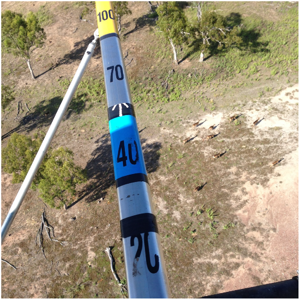
Following Gentle and Pople (2013), surveys were flown with the two rear and front left doors removed at a ground speed of 93 km h−1 (50 kts) and at a height of 61 m (200 ft) above ground level. Observers used a voice recorder to record groups (or clusters) of animals seen in distance classes perpendicular to the helicopter. Time of sighting was recorded automatically. Distance classes (0–20, 20–40, 40–70, 70–100, 100–150 m) were identified on aluminium poles extending from both sides of the helicopter (Fig. 3). Surveys were flown in daylight within 3 h of sunrise or sunset when deer are more likely to be active and in open areas and, therefore, detectable compared with the middle of the day (Bengsen et al. 2022; Forsyth et al. 2022). Two rear observers were used on all surveys. When weight restrictions permitted, a front-left observer was included in a survey session, allowing simultaneous counts on the left side, which could be analysed using mark–recapture distance sampling (MRDS; Burt et al. 2014; see below). Four observers were used during the surveys and two or three were assigned to seating positions randomly for each survey session.
Chital deer group (or cluster) passing under a survey boom attached to a Robinson R44 helicopter. Numbers on the boom refer to distance intervals on the ground perpendicular to the helicopter. Photograph credit: M. Amos.
Distance data collected by the rear observers were analysed using multiple covariate distance sampling (MCDS; Marques et al. 2007) in DISTANCE 7.3 (Thomas et al. 2010). MCDS estimates density by adjusting counts for detection probability, which is determined by modelling the decline in detection probability with distance from the transect line. MCDS analysis involves fitting a detection function to the perpendicular distances for all observations and including covariates such as stratum, vegetation cover and observer. In MCDS, covariates affect the scale rather than the shape of the detection function (Marques et al. 2007). MCDS can be particularly useful when there are too few sightings (<60; Buckland et al. 1993) to model separate detection functions for each stratum such as a property. In that case, a detection function is fitted to data from all strata and a factor covariate is included with a level for each stratum. In the analyses here, factor covariate levels were often grouped to provide a simplified model and to increase sample size. The minimum sample size for factor covariate levels in this study was n = 20. Potential detection functions available in DISTANCE comprise a key function (half-normal or hazard-rate) with, if necessary, a cosine, polynomial or Hermite series expansion to adjust the key function to improve model fit (Buckland et al. 1993). Models are fitted to survey data and the most parsimonious model is selected using minimum AICc. Detection functions also needed to meet the shape criterion of a ‘shoulder’ near the transect line (i.e. constant detection probability = 1 close to the transect line; Buckland et al. 1993).
For the 2014 aerial surveys, separate models were fitted with a covariate for location (two levels: region (Fig. 1b) contrasted with the two properties and Maryvale Creek combined; or four levels: region, Maryvale Creek, Niall and Spyglass separately) or no covariates. Locations differ in vegetation cover, which is likely to influence detection probability (Laake et al. 2008; Forsyth et al. 2022). The average size of detected clusters may be biased if large clusters are more likely to be detected at greater distances. Average cluster size was therefore adjusted by regressing loge(cluster size) against g(x), the probability of detection at perpendicular distance x from the transect line (Buckland et al. 1993), if the regression was significant at P < 0.15, which is a conservative option provided in DISTANCE. MCDS assumes that the probability of detecting a deer cluster on the transect line g(0) is certain (i.e. g(0) = 1). MRDS can estimate g(0), which can then be used to adjust the MCDS density estimate as a multiplier in DISTANCE (Thomas et al. 2010).
Distance data collected by the left-side observers were analysed using MRDS in DISTANCE 7.3. On the basis of recorded times, sightings were separated into those seen by both observers and those seen only by the front observer or only by the rear observer. Categorisation of duplicate sightings followed Fewster and Pople (2008). MRDS was used solely to determine an estimate of g(0) by using its mark–recapture component, with little interest in its distance-sampling component involving modelling detection probability away from the line. MCDS density estimates using data from the two rear observers in the previous analysis could then be divided by g(0) to best estimate true density (Laake et al. 2008). For the distance-sampling component, detection probability was modelled using a half-normal key function with no covariates. For the mark–recapture component, small sample size limited the analysis to separate models fitted with one of two covariates, observer position (front or rear) or perpendicular distance. These were compared along with a model with no covariates by AICc. Point independence was assumed (Burt et al. 2014).
Vehicle ground surveys on Spyglass and Niall
The density of chital deer was monitored one to four times per year on Spyglass during November 2013–March 2022, and on Niall during December 2014–May 2020 by using vehicle ground surveys along property tracks (see Fig. S2). Standing on the tray back of a utility four-wheel drive vehicle, a single observer recorded perpendicular distances to clusters of deer and the cluster size on either side of the vehicle driven between dusk and midnight at ~20 km h−1. Sightings were recorded into a voice recorder with the aid of a spotlight, rangefinder and binoculars. The same observer was used for all surveys. Perpendicular distances were converted to intervals (0–10, 10–20, 20–40, 40–70, 70–100, 100–150, 150–200 m) prior to analysis, to reflect approximations at greater sighting distances and truncating at 200 m. Chital deer have relatively bright eyeshine and are readily seen out to 200 m in a spotlight beam, but binoculars are often required to confirm cluster size. Approximately 50 km was driven along nine transects on Niall (see Fig. S2). These occurred in separate woodland and creek geographic strata, with deer at higher density in the latter (see Fig. S2). Approximately 50 km was also driven along six transects on Spyglass. These were not stratified but spanned the width of the southern end of the property between two sets of homesteads. Placing a 1 km buffer around the Niall transects gave an area sampled of 92 km2. The buffer distance is approximately half the distance between adjacent transects and is consistent with the decline in chital deer abundance with an increasing distance from homesteads (Forsyth et al. 2019).
Distance-sampling data were again analysed using MCDS as above, but assuming g(0) = 1. For Niall, vegetation type (creek or woodland) was included as a covariate and compared with the model with no covariates by AICc. A property density estimate (±s.e.) was calculated from combined stratum estimates (McCallum 2000). For Spyglass, two and four levels of vegetation density (open–dense) were included as covariates and compared with a model with no covariates by AICc. For both properties, average cluster size was again adjusted by regressing loge(cluster size) against g(x).
Numerical response
Rainfall is often used as a surrogate for food supply in describing herbivore dynamics in the Australian rangelands (e.g. Gentle et al. 2019; McLeod et al. 2021). Alternatives are to measure pasture biomass directly or model it. The latter was employed here, with total standing dry matter (TSDM) in the study areas extracted from FORAGE (https://www.longpaddock.qld.gov.au/forage/; Zhang and Carter 2018). Within FORAGE, TSDM is modelled by GRASP (McKeon et al. 1990), which uses daily weather data, vegetation type, tree density, livestock stocking rates, and kangaroo and feral herbivore densities. GRASP was developed for northern Australian grazing systems such as on Spyglass and Niall, which are dominated by perennial grasses. AussieGRASS (Carter et al. 2000) is used by FORAGE to run GRASP simulations in 5 km × 5 km grid cells across the continent.
Average monthly TSDM on Spyglass during 1975–2021 was 919 kg ha−1, but was highly variable (CV = 66%; median monthly TSDM = 723 kg ha−1). As with rainfall, TSDM on Spyglass showed a strong seasonal cycle, but with marked year-to-year differences (Fig. 2b; similar TSDM was simulated for Niall and is provided as Fig. S1b). However, there are clear trends over the study period, with TSDM on both properties declining from a high in mid-2011 to a low in December 2015. The TSDM minima recorded in the study period were the lowest recorded during 1975–2022. From those minima, TSDM increased over the long term, but remained below the long-term average on both properties.
The relationships between exponential rate of increase (adjusted for culling, see below) between surveys on Spyglass and Niall and past rainfall and TSDM were explored graphically and through correlation. The number of deer culled in the buffered area on Niall in 2014 and 2016 was determined from GPS fixes (see below) or locations of kills recorded by shooters. Rainfall periods assessed were the 6 and 12 months of rain falling prior to the second of two consecutive density estimates used to calculate the rate of increase (i.e. no time lag), and 12 months of rain with a 6- or 12-months time lag. TSDM was assessed at times with no time lag, and with a 6-months and 12-months time lag prior to the second density estimate.
The rainfall interval and past TSDM with the strongest correlation and logical relationship with annual exponential rate of increase were used to model the numerical response (Choquenot 1998; Gentle et al. 2019). An asymptotic exponential model was fitted to the data in R 4.0.5 (R Core Team 2021) by using the function nls. The model takes the form
where r is annual exponential rate increase, a is the horizontal asymptote (i.e. maximum r), b = a – R0 (where R0 is the y-axis intercept and minimum rate of increase), c is the logarithm of the rate constant and x is rainfall or TSDM (Crawley 2013). Models with rainfall and TSDM were compared by AICc. This model has been used to describe the numerical response of large herbivores to proxies of food supply in the Australian rangelands (Cairns and Grigg 1993; Gentle et al. 2019). Ivlev’s inverted exponential has also been used (Bayliss 1987; Caley 1993; Choquenot 1998) and returns the same curvilinear relationship.
Property-based culling and aerial surveys
Aerial and ground-based culling of chital deer by professional shooters was undertaken on several properties during 2016–2018. The helicopter-based shooting is described by Bengsen et al. (2022). Ground-based shooting occurred on Niall and Felspar in November 2016, after the aerial culling. Deer were shot from a utility four-wheel drive vehicle at night by using hand-held and vehicle-mounted spotlights. The culling followed the national code of practice for the destruction or capture, handling or marketing of feral livestock (Standing Committee on Agriculture, Animal Health Committee 2002; Hampton et al. 2022) and complied with the Queensland Animal Care and Protection Act 2001. Permits were not required to cull feral deer on private land because they are declared as ‘restricted matter’ in the Queensland Biosecurity Act 2014 and were taken as part of a control program. Aerial surveys using the methods described above were flown prior to culling to determine the percentage of the population removed. Recreational hunting of chital deer occurred on all six properties, but the removals were not recorded. An exception was on Niall, where recreational hunters culled 534 deer over 5 days in December 2014.
Abundance estimates and the number of deer culled are reported for four properties that were surveyed by helicopter, namely, Niall, Maryvale, Felspar and Gainsford (Fig. 1b). Two other properties, Toomba and Lowholm, were not part of the culling program but were surveyed for comparison and to monitor regional trends. The 20 km transect along Maryvale Creek was again flown in 2016. The six properties plus Spyglass are cattle grazing properties that range in size from 86 km2 to 672 km2. Aerial surveys were flown in the week prior to culling. Chital deer are concentrated in areas of <4 km from homestead in the region (Forsyth et al. 2019) and this was confirmed by landholders who described the distribution on each property. On Niall and Felspar in 2016, parallel transects were 500 m apart. On the basis of landholder descriptions, surveys on other properties were stratified into high- and low-density areas by using a mixture of parallel transects 500 m and 300 m apart, with care taken to avoid counting animals twice. The culling team recorded the location of kills and GPS tracks to ensure that they fell within the surveyed area. Surveyed and therefore culled areas were 40 km2 (Niall), 14 km2 (Maryvale), 15 km2 (Felspar), 10 km2 (Gainsford), 16 km2 (Toomba) and 16 km2 (Lowholm).
In August 2020, surveys were flown with an Airbus AS350 SD1 Squirrel helicopter at the same height and speed as above. Three observers randomly assigned to seats were used on all surveys, allowing MRDS on the left-hand side. Angles to deer clusters were determined using inclinometers and perpendicular distances were subsequently calculated using the survey height and trigonometry. Sighting data were again recorded directly into voice recorders. Surveys were flown on Maryvale, Felspar, Gainsford, Toomba, Lowholm and the single transect along Maryvale Creek. A stratified survey design was again used, but with zigzag rather than parallel transect lines to improve efficiency (Buckland et al. 2015). Surveys were also flown in the same month on Spyglass and another site on Rita Island 50 km south of Townsville by using identical methods and the distance and mark–recapture data were used to supplement the MRDS and MCDS data in this study.
The 2016–2018 distance data were analysed using MCDS and, as only two rear observers were used, the resulting density estimates were corrected using g(0) calculated from the 2014 survey. Year (three levels), property (five levels, excluding Lowholm), observer team (three levels) and combinations of these were included as covariates and compared with the model with no covariates by AICc. Lowholm had too few sightings (n = 2) to be included as a property factor level. A separate MCDS analysis was therefore undertaken including Lowholm and with only year, observer team or both as covariates and compared with the model with no covariates by AICc.
For the analysis of the 2020 survey, MCDS was used with property (two levels: properties and Rita Island; or four levels: Rita Island, Toomba, Spyglass, other properties), observer team and combinations as covariates and compared with a model with no covariates by AICc. In 2020, g(0) was calculated from a separate MRDS analysis, again by using a half-normal key function with no covariates for the distance-sampling component because the focus was on the mark–recapture component. Sightings by the left-side observers were categorised as for the 2014 survey above. For the mark–recapture component, separate models were fitted with either observer position (front or rear) or perpendicular distance as covariates. These were compared along with the model with no covariates by AICc. Point independence was again assumed.
Fecundity
At least 10 adult male and 10 adult female chital deer were shot and dissected to determine morphometrics and seasonal reproductive status and body condition (Queensland Department of Agriculture and Fisheries Animal Ethics permit number: SA 2014/07/475) in October 2014, March and October 2015, and March 2016 on Niall and Spyglass. Deer were placed in one of six age categories (<1, 1–2.5, 2.5–4, 4–6, 6–8 and ≥8 years old) determined from tooth eruption and wear (Buchholz 2022) in the laboratory by the same observer. Tooth eruption indicates deer age up to 3 years old in chital deer (Graf and Nichols 1966; Buchholz 2022), but tooth wear tends to underestimate the true age of older animals particularly ≥6 years old (Foley et al. 2022). Factors such as location, diet and observer biases are believed to influence deer age estimated from tooth wear, but the influence can be minor (Hamlin et al. 2000; Foley et al. 2022). For Texan chital deer, Buchholz (2022) found deer age in ≥2-year age groupings determined by tooth eruption and wear matched ages determined by cementum annuli, which is regarded as the most accurate measure available (Hamlin et al. 2000; Foley et al. 2022), and that tooth wear did not differ between the sexes. For this study, deer were sampled from the same geographic area, animals ≥8 years old were placed in a single age class and age was used as a relative rather than an absolute measure in comparisons between the sexes. Fetuses were weighed and aged using an equation developed by Kelly et al. (2022) from the relationship between fetal weight and age described for Hawaiian chital deer (Graf and Nichols 1966). Lactational status was determined by palpating teats. This sample of the number of fetuses per adult female was supplemented by 63 pregnant females from aerial culls on properties in the region during 2016–2018 described above. These were animals (n = 192), including males, that could be conveniently brought from where they were shot to a central processing location. They represented ~20% of the total number culled on properties.
Assessment of breeding success was made by determining the proportion of adult females that were breeding to full potential (BFP) on each sampling occasion. This statistic combines the pregnancy and lactational status of adult females. A female that is pregnant and lactating is BFP. Given the below estimates of weaning age and parturition–conception interval, a female with a fetus of >4 months old will not be lactating and so is considered BFP. Females in other states are considered not BFP. This underestimates the proportion that is BFP because there are 48 days in a year (i.e. 0.13 probability) when a female BFP is neither pregnant nor lactating.
Data were analysed by logistic regression in R 4.0.5 by using the proportion of females that are BFP as the response variable, with property, season and their interaction as explanatory variables using routine glm with binomial errors. Rainfall in the 6 months and 12 months prior to sampling and TSDM at the time of sampling were also included separately as explanatory variables. Models were checked for overdispersion (Crawley 2013), and AICc was used to compare models.
Maximum rate of increase
An estimate of the maximum exponential rate of increase of a chital deer population was made using the Euler–Lotka equation (Caughley 1977; McCallum 2000), as follows:
where r is annual exponential rate of increase, x is age, mx is annual fecundity (female offspring per female per year) and lx is survivorship to age class x + 1. This was solved numerically for r by using ‘Goal Seek’ in Microsoft Excel (McCallum 2000). With unlimited resources, vital rates should approach their physiological maximum for a particular environment and r will approximate rm. Fecundity was based on the following data collated by Ernest (2003): gestation is 235 days, weaning at 4 months, and females first reproduce at 12.64 months (cf. 11 months used by Hone et al. (2010)) and litter size is 1.03. The latter was estimated separately for the study area, as explained above. Information also required to estimate fecundity is that conception can occur as soon as 48 days after parturition in both captive and wild populations (Graf and Nichols 1966; English 1992). A range of values was used for adult (0.85–0.95) and juvenile (0–1 years old; 0.75–0.85) survival, which fall within the ranges recorded for female large mammals compiled by Gaillard et al. (2000). All animals were assumed to have died by their 21st birthday, which was the maximum lifespan reported by Ernest (2003). Female sexual maturity has been recorded as early as 10 months in the wild (Graf and Nichols 1966) and captivity (English 1992). This value was also used along with an estimate for litter size from the study area to provide an alternative estimate for rm.
The rm value as calculated above is for only the female component of the population with a stable age distribution. The actual rate of increase of the population may be higher if it is biased towards mature females. The sex ratio of the deer populations ≥1 year old on the four culled properties plus two others was therefore also determined from samples of culled animals during 2016–2018 (n = 163). These samples are assumed to be random because the shooter was non-selective as was their retrieval. However, larger, usually male deer may have been more detectable and more likely to be shot and retrieved. The sex ratio of samples of culled animals was compared with parity by using a sign test. Logistic regression models with sex ratio varying across the 3 years and with no year effect were fitted using the function glm with binomial errors in R 4.0.5. Models were compared using AICc. Average age of the sexes was compared with a Student’s t-test and the age distributions of the two sexes were compared using a Kolmogorov–Smirnov test.
Results
Broad-scale aerial survey
In 2014, MRDS was possible on 250 km of broad-scale and 60 km of additional survey transects. The MRDS model with best support included no covariates (see Table S1a) and estimated g(0) (±s.e.) as 0.72 ± 0.08. For MCDS, only 37 clusters of deer were recorded on the broad-scale aerial survey. Fortunately, a further 134 clusters were recorded on additional surveys to provide a sufficient sample size for modelling the detection function. The MCDS model with most support used a half-normal key function with no series expansion and included a covariate for location with four levels (see Table S1b). Including g(0) as a multiplier, density (±s.e.) for the broad-scale survey region was estimated as 3.91 ± 2.04 deer km−2. As the poor precision suggests, deer were patchily distributed in the landscape. Deer were seen on only four of the nine transects. Across all survey locations, only 2 of 171 clusters of deer were seen >5 km from homesteads. In contrast, eastern grey kangaroos (Macropus giganteus) and cattle were both seen on all transect lines and throughout the landscape. The clumped dispersion of deer in the landscape was particularly striking on the Maryvale Creek transect where there were 177.9 ± 35.5 chital deer km−2. Deer were not recorded >2 km away from the creek on the 672 km2 Maryvale property.
Vehicle ground surveys on Spyglass and Niall
Deer on both Niall and Spyglass are known to be close to homesteads (Forsyth et al. 2019). On Spyglass, there was considerable spatial variation in deer abundance, with transects close to the homesteads recording high densities, and those away from homesteads recording low densities (see Fig. S2). This led to poor precision in the density estimates (CV mean = 50%, range 32–84%). On Niall, this problem could be addressed to some extent through stratification (CV mean = 41%, range 22–68%). For Spyglass, the MCDS model with most support used a hazard-rate key function with no series expansion and included a covariate for vegetation density with two levels (see Table S2a). For Niall, the best model was also a hazard-rate key function with no series expansion but with no covariates (see Table S2b).
Only four transects (22–24 km) could be driven on Niall in December 2018 and February 2020 because of muddy roads. To avoid bias, density based on transects driven on those occasions was multiplied by a correction factor = (mean density of all occasions using all transects) / (mean density of all occasions using the four transects always driven). This was performed for the two strata separately. The correction factor was based on data from all occasions except December 2018 and February 2020.
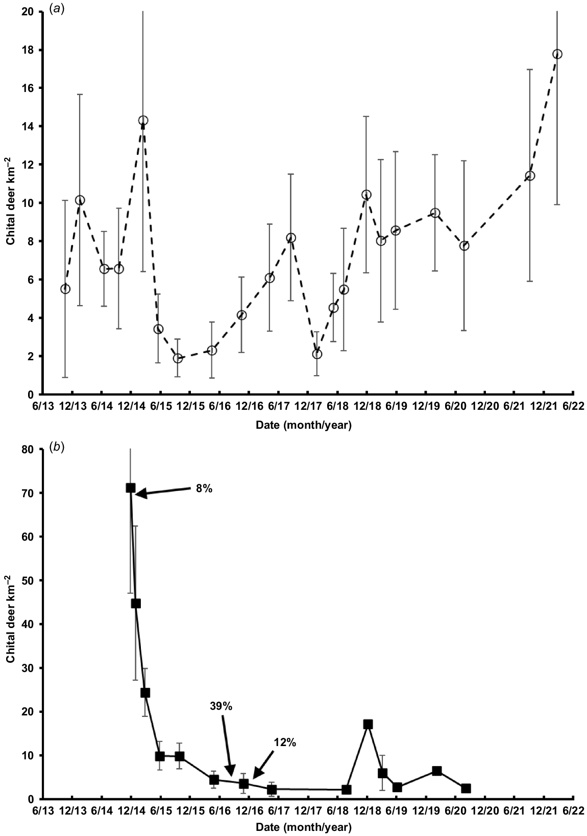
The dominant feature of the dynamics of the chital deer populations on Niall and Spyglass was a dramatic decline on both properties during early 2015 (Fig. 4). From March to October 2015, chital deer declined (±s.e.) by 87% (annual r = −3.68 ± 2.80) on Spyglass and, from January (after the recreational cull) to October 2015, the Niall population declined by 78% (annual r = −2.05 ± 1.00). The three recorded culling events on Niall are shown as percentages in Fig. 4. The removal of over 500 animals in late 2014 represented only 8% of the population. Higher rates of removal were recorded at lower densities following the drought decline. The Niall population generally remained at <10 deer km−2 up to late 2020. In contrast, the population on Spyglass recovered, with some fluctuation, to its pre-drought density by 2021–2022 (October 2015–March 2022: annual r = 0.35 ± 0.24).
Density (mean ±s.e.; individual deer km−2) of chital deer on (a) Spyglass and (b) Niall, both being based on night-time vehicle ground surveys with a spotlight. Two upper error bars in (a) and one error bar in (b) have been truncated for clarity. The percentage of animals culled on Niall either side of a density estimate is given, and the timing is indicated by arrows.
Numerical response
Estimated rates of increase among surveys were highly variable (Fig. 4) with no obvious relationship with rainfall or TSDM when plotted. Rates of increase were therefore calculated between annual density estimates each year, calculated by interpolating the two survey estimates straddling 1 July. The first and last survey estimates of the time series were extrapolated 3–4 months to the preceding or following 1 July. These annual estimates essentially smoothed the time series.
Using data from both properties, the strongest, positive and significant correlations were with 12-months rain with no time lag (t = 3.67, d.f. = 13, P < 0.01) and with TSDM with no time lag (t = 3.60, d.f. = 13, P < 0.01) (see Table S3). This was logical, given that rainfall period had the strongest correlation with TSDM of the four periods examined (t = 3.95, d.f. = 13, P < 0.01).
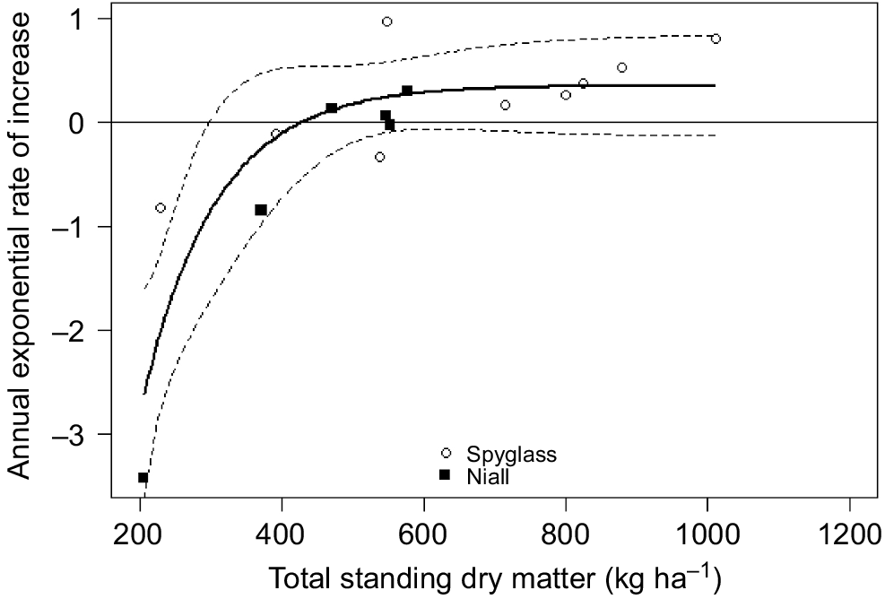
The asymptotic exponential model provided a reasonable description of the numerical response of chital deer to TSDM (Fig. 5). There was a greater scatter of points around the modelled relationship with rainfall and a poorer spread of rainfall values (see Fig. S3). The better AICc of the rainfall-driven model (24.5 vs 29.3) was thus misleading, and so the model with TSDM was preferred. Only the parameter c was significant (Table 2). The x-axis intercept indicated that the population increases at TSDM of >427 kg ha−1. This value is less than half of the long-term average.
Annual exponential rates of increase of chital deer on Spyglass (open circles, 2013–2022) and Niall (solid squares, 2014–2020) plotted against TSDM (kg ha−1) at the time of the second survey used to calculate rate of increase. The solid line is a fitted asymptotic regression. The dashed lines are the 95% confidence intervals fitted using package investr (Greenwell and Kabban 2014) in R 4.0.5. See text for details and Table 2 for model parameters.
| Coefficient or statistic | Estimate |
|---|---|
| a | 0.35 ± 0.22 |
| b | 20.84 ± 20.49 |
| c | −4.65 ± 0.48*** |
| R0 | −20.49 |
| Residual standard error | 0.55 |
***P < 0.001. See text for details.
The sharp drought decline on Niall stands out as an isolated point in Fig. 5, clearly influencing the low estimated minimum exponential rate of increase (R0; Table 2). Notably, the asymptote was ~0.35 (Table 2), which matches the annual exponential rate of increase observed for the population recovering from drought on Spyglass and matches the upper end of the range for rm estimated from the Euler–Lotka equation (see below).
Property-based culling and aerial surveys
For the 2016–2018 surveys, the best MCDS models with and without Lowholm used a hazard-rate key function with no series expansion and year as a covariate (see Table S4). In 2020, the distance data were truncated at 100 m to simplify modelling, given there were few detections >100 m (Buckland et al. 2015). The MRDS model with best support by using 2020 data included no covariates and estimated g(0) as 0.53 ± 0.05 (see Table S5a). The best MCDS model was a half-normal key function with no series expansion and with no covariates (see Table S5b).
The 2016 aerial survey of the Maryvale Creek transect remarkably recorded no deer. The decline on that transect (annual r = −3.12 ± 0.62, using a density of 0.1 deer km−2 for 2016) was almost identical to that recorded on Spyglass, and similar to that on Niall (Fig. 6a; see above). In all sites without professional culling, the density of deer increased following surveys from October 2015 (Fig. 6a). The annual exponential rates of increase (r) to 2020 were 0.29 ± 0.22, 0.46 ± 0.20, 0.70 ± 0.52 and 1.57 ± 0.37 for Spyglass, Toomba, Lowholm and Maryvale Creek (again using 0.1 deer km−2 for 2016) respectively.
Density (mean ±s.e.; individual deer km−2) of chital deer on logged y-axes for (a) sites not culled by professional shooters, (b) culled properties Felspar and Niall, and (c) culled properties Gainsford and Maryvale. For (b) and (c), culling is indicated by a vertical arrow and represented 8%, 39% and 12% of the population on Niall, 67% and 49% on Felspar, 55% and 88% on Gainsford and 76% and 84% on Maryvale. The initial culling on Niall is obscured, but is shown in Fig. 3.
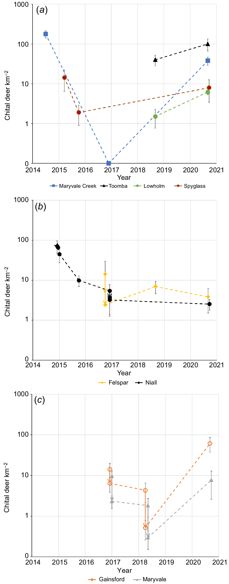
Population reductions of 55–88% by aerial and ground-based culling over 1–2 days were recorded on Felspar, Gainsford and Maryvale (Fig. 6b). Reductions of 8–39% by aerial and ground-based culling over 1–5 days were recorded on Niall. However, this reduction was for an area (92 km2) monitored by vehicle surveys that was larger than the area culled. The aerial-culling component removed 49% of the population on Niall and an adjoining property in 60 km2 covered by an aerial survey (Bengsen et al. 2022). There were strong recoveries during 2018–2020 on Gainsford (annual r = 1.97 ± 1.25) and Maryvale (annual r = 1.37 ± 1.13), in contrast to Niall and Felspar, where there was little or no increase (Fig. 6b).
Fecundity
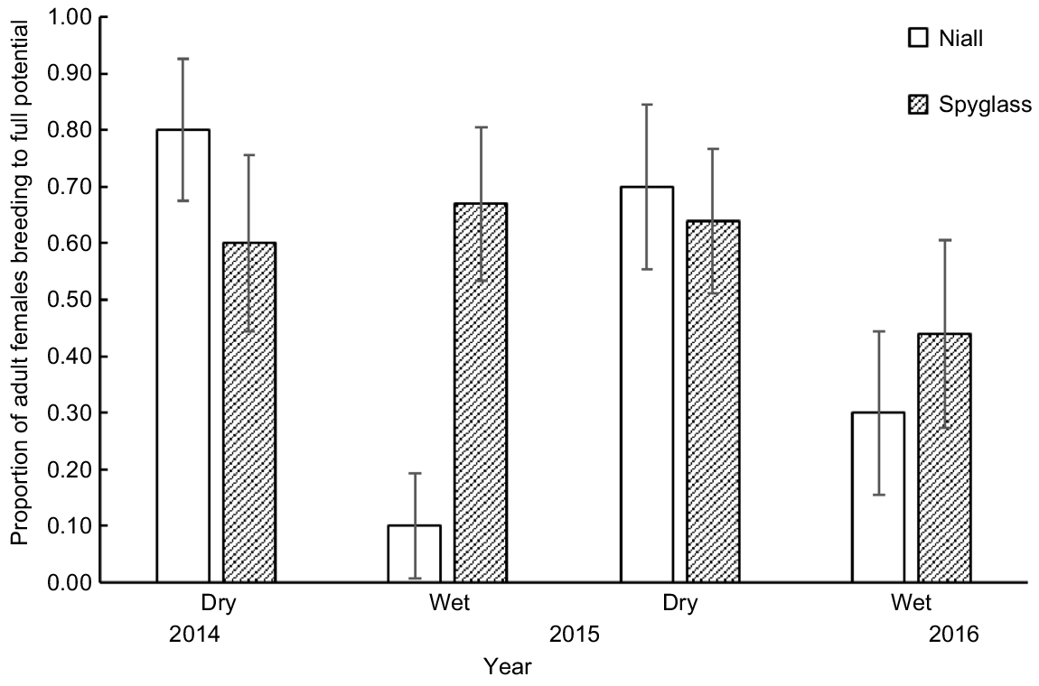
The best logistic regression model predicting the proportion of females BFP included season as a covariate, whereas rainfall in the 6 months prior to sampling had some support (ΔAICc = 2.7; see Table S6). The proportion of females BFP was lower on Niall and during the wet seasons in 2015 and 2016 (Fig. 7). Only 10% of females were pregnant in the 2015 wet-season sample and no females were lactating on either property in the 2016 wet-season samples.
The proportion (±s.e.) of adult females breeding to full potential on Niall and Spyglass from four seasonal shot samples during 2014–2016.
Only one set of twin fetuses was recorded from 116 shot pregnant females. That equates to a litter size of 1.01, which is almost identical to that documented by Ernest (2003).
Maximum rate of increase
The Euler–Lotka equation returned a range for rm of 0.229–0.347, reflecting the lower and upper ranges of juvenile (0.75–0.85) and adult survival (0.85–0.95) that were used. This range for rm is equivalent to finite rates of increase of 1.26–1.41. Using both 10 months as female age at first reproduction and a litter size of 1.01 made virtually no difference to the estimate of rm (= 0.235–0.352; i.e. changes in the two parameter estimates cancelled each other out).
The culled samples of the population ≥1 year old were significantly female biased (0.60 female, 95% CI 0.52–0.68), but the adult age distributions did not differ between the sexes (D = 0.10, P > 0.8, n = 98 females and 65 males). There was no difference in the average age of the two sexes in the culled samples (t = 0.03, d.f. = 144, P > 0.9). The model with sex ratio varying across the 3 years was not supported by quasi-likelihood AICc (QAICc), which was used because the data were overdispersed (Burnham and Anderson 1998; Crawley 2013; see Table S7).
Discussion
Declines in chital deer populations in northern Queensland during drought have been reported previously (Jesser 2005) but are quantified here. Large declines of ~80% over 7–10 months were recorded on three sites in this study. Animals were in poor body condition in the dry seasons of 2014 and particularly 2015 on Spyglass and Niall (Watter et al. 2019a), consistent with mortality of adult deer. Female reproductive status indicated that recruitment was minimal during this period, but this was of secondary importance to the decline, which would have been driven by adult mortality. For Australia, these data are a reminder that not all deer populations are increasing inexorably, as suggested by monitoring data for some temperate populations (e.g. Eco Logical Australia 2015; Cunningham et al. 2022; Moloney et al. 2022), and that large herbivore populations in the dry tropics can fluctuate considerably. Indeed, the population dynamics seen here in chital deer, characterised by steep drought declines and lengthy recoveries, is like that seen in other large herbivore populations in the semi-arid and arid zones of Australia (Pople and Froese 2012; Gentle et al. 2019; McLeod et al. 2021). Fluctuations in large herbivore abundance occur for reasons other than rainfall-driven food supply, such as predation, disease and winter severity (Sæther 1997; Ogutu and Owen-Smith 2005). Such labile dynamics contrast with populations remaining at roughly a constant size from year-to-year and populations increasing at a constant rate annually when introduced to a new environment or released from a limiting factor (Forsyth and Caley 2006).
Drought is also a feature of temperate Australia. In Tasmania, fallow deer (Dama dama) increased at an annual exponential rate of r = 0.11 over a 35-year period, but this included a decline over ~4 years during a period of below-average rainfall (Cunningham et al. 2022). Fallow deer on the Northern Slopes region of New South Wales apparently persisted during drought when livestock were destocked, and deer were consuming browse (Davis et al. in press). Drought would have reduced the rate of increase of fallow deer at the time, but this will again likely be hidden in their longer-term positive rate of increase and spread (Crittle and Millynn 2020).
Fluctuations in population size have at least two consequences for large-pest herbivorous mammals (>30 kg; Caughley and Krebs 1983). Large body size is relevant because it is associated with relatively low rates of increase and suggests that a species will be extrinsically regulated by resources external to the animal rather than intrinsically through interactions among individuals of a population through spacing behaviour (Krebs 2009). The first consequence is that concern over perceived likely impacts also fluctuates, increasing on the upswings in pest abundance and when livestock and wildlife food supply becomes limiting. Second, a decline brings a strategic opportunity to efficiently control large herbivores such as chital deer and the culling in this study was undertaken at an appropriate time. The exception was the 534 animals removed prior to the decline on Niall at a time of increased concern from the landholder over deer impacts, although the subsequent decline in chital deer abundance could not be predicted at the time. Modelling by Pople and McLeod (2000) showed that the same removal rate of animals from a red kangaroo (O. rufus) population will result in the greatest long-term reduction when applied immediately after rather than prior to a drought decline. Culling after the drought is cost effective because fewer animals are removed and the population recovery can be substantially delayed. However, the decline and recommended delay in control may not be predicted with sufficient confidence to offset heavy grazing pressure by pest herbivores. Grant funding for feral-pest control has been provided in the past to take advantage of the lowered pest density and concentration around water points during drought (Pople et al. 1998).
Despite the declines to low density, chital deer populations recovered from both drought and culling at rates of increase close to or higher than the maximum rate, but the pre-drought density was not reached until ~6 years later at least on Spyglass. Rates of increase higher than rm may have been due to a female-biased sex ratio but also due to immigration. Surveyed areas were small (10–40 km2), so the populations were certainly open to movements into or out of the study area. However, aerial surveys over a broader area on each of the six properties recorded few or no deer (authors, unpubl. data), which is consistent with the findings of Forsyth et al. (2019). Chital deer remained at lowered densities on two culled properties, namely Felspar and Niall. On both properties, there was recreational culling, possibly at a higher rate than on other monitored properties, and this may have been sufficient to stop the population from increasing. Rapid rates of increase in chital deer populations have been recorded elsewhere (Duckworth et al. 2015; Gürtler et al. 2018) and are consistent with the rates recorded here, with immigration contributing to the increase.
While reproductive output was depressed in early 2015 and 2016, it is unclear why it was lower on Niall than Spyglass. Fecundity could not be explained by a simple relationship with rainfall or TSDM. Both properties experienced similar rainfall and TSDM deficits and subsequent population declines. Livestock numbers may have differed among properties but were not recorded. Body condition as measured by kidney fat index was similarly low on both properties in the dry seasons of 2014 and 2015 (Watter et al. 2019a). Although rainfall and TSDM were almost identical on the two properties, better-quality food on Spyglass, even if only in a refuge, may have enabled the population to start recovering from October 2015, whereas the population continued to decline on Niall (Fig. 4).
Food is not the only limiting factor for chital deer in northern Australia. Chital deer were recorded in 28% of dingo scats collected on Niall and Spyglass (cf. 8% of dingo scats in Victoria with sambar deer; Forsyth et al. 2018) and in almost all scats <1 km from homesteads, and dingoes were regularly seen on remote cameras on Niall (Forsyth et al. 2019). Although speculative, dingoes may be able to regulate chital deer once they are reduced to low density and may have contributed to suppressing growth on Niall and possibly Felspar. Using cameras, a high abundance index for dingoes was recorded on Niall, and to a lesser extent Felspar, compared with Spyglass in the study of Forsyth et al. (2019). The high chital deer densities recorded pre-drought and in 2020 suggest that dingoes were a minor limiting factor and certainly not regulating populations at those times. Following Sinclair and Pech (1996), limitation refers to the process (via mortality and reproduction) that sets a potential equilibrium population density, whereas regulation is the density-dependent process that pushes a population towards that equilibrium density.
The distribution of deer in the 2014 broad-scale aerial survey was consistent with the clumped dispersion of chital deer around homesteads on seven properties recorded by Forsyth et al. (2019). Long transect lines (Fig. 1a), as used in the 2014 aerial survey, are inappropriate to monitor the regional population. A better option is to monitor the area around homesteads on several properties as was undertaken here. Properties with few or no chital deer would also need to be monitored. The aggregation of chital deer populations around homesteads appears at least partly due to the distribution of essential minerals such as phosphorus, sodium and zinc (Watter et al. 2019b). Why these minerals should be concentrated around homesteads is unclear. Chital deer are also generally recorded only within 3 km of a waterpoint such as a farm dam or trough (Forsyth et al. 2019). This concentration around water and homesteads, which is likely to be pronounced during the dry season, also provides a strategic opportunity for control, in addition to reduced population size in drought. These areas are relatively small and so only small absolute numbers would need to be removed, particularly after drought for effective control. The large declines in chital deer populations during periodic droughts, coupled with their clumped dispersion around homesteads and occurrence on only some properties may contribute to their apparent slow spread from their point of release in the 1880s (Watter et al. 2019a). Their expansion would require ‘hopping’ between islands of suitable habitat. However, even if the rate of spread has been 1 km per year (see Introduction), this is close to the median dispersal rate of 1.29 km per year (range 0.64–8.69) for nine species of ungulates following their introduction to New Zealand (Caughley 1963).
An rm of 0.35 is slightly higher than that for red kangaroos (0.29, Pople et al. 2010), which have a single young per birth, but lower than that for feral goats (0.50, Pople and Froese 2012) and feral pigs (0.69, Choquenot 1998), with the latter two species having multiple young per birth. This estimate of rm for chital is thus logical by comparison and more realistic than the estimate of Hone et al. (2010). The difference is explained by the latter being based on a relationship derived for the Artiodactyla rather than the species-specific calculation made here. The Euler–Lotka equation is deterministic and so will overestimate the growth of a population with stochasticity in its survival and fecundity schedule (Tuljapurkar and Orzack 1980), and so a range of values for rm is presented here. Regardless of whether potential rates of increase are higher than rm owing to female bias in the sex ratio or immigration, to stop population growth requires culling each year at the rate the population would otherwise increase. The instantaneous rate rp = loge(Nt + 1/Nt), where rp is the potential rate of increase, is the appropriate rate to cull a population throughout the year, such as by recreational hunters. If there is a single cull, then the appropriate rate is the isolated rate, which is 1−e−rp (Caughley 1977). For an rp equal to an rm of 0.35, the isolated rate is ~0.30.
The post-drought population of chital deer was female biased (0.60 female), which is consistent with many studies of survival patterns in ungulates and other taxa (Sæther 1997; Owens 2002; Toïgo and Gaillard 2003). Drought is likely to have accentuated the bias, with larger-bodied male chital deer at a greater disadvantage during the nutritional shortfall. Surprisingly then, male and female age distributions were similar, but a larger sample size would be needed to detect differences in particular age classes.
Frustratingly, density estimates on both Spyglass and Niall had poor precision, reflecting considerable spatial variation in deer abundance among transects. As Bengsen et al. (2022) suggested, density surface models (Miller et al. 2013) are an option to improve precision here. The poor precision translated to the estimated rates of increase and would have compromised quantifying a relationship between rate of increase and rainfall or TSDM. However, the effect of rainfall was obvious, with declines recorded when 12-months rainfall was <400 mm (see Fig. S3). That rain fell between the two abundance estimates used to determine the rate of increase, and would have directly affected food quality and quantity available to animals, logically influencing their survival and reproductive output.
Using TSDM as the explanatory variable provided a more direct and convincing relationship between the rate of increase and food supply. Directly measuring rather than simulating pasture biomass may have improved the relationship with the rate of increase. Direct estimates of livestock, kangaroo and feral herbivore density rather than using regional averages could also have improved the relationship. In their native range, chital deer populations appear to be sensitive to livestock grazing, with populations increasing when livestock are reduced (Duckworth et al. 2015).
It is surprising that the numerical response function did not record negative exponential rates of increase until TSDM was well below the long-term mean. For both rainfall and TSDM, the median is probably a better benchmark than the mean, given the occasional very high rainfalls and periods of high TSDM that would have inflated the means. However, the median is still well above the value where the numerical response function crossed the x-axis. The model indicates that chital deer populations in the region are capable of lengthy periods of increase, interrupted by declines when food supply is well below average. The trajectory of the deer population therefore must be seen in the longer term, emphasising the point made earlier. Parameters a and b in the numerical response model were non-significant, as reported by others (Cairns and Grigg 1993; Gentle et al. 2019), suggesting a simpler model could have been fitted. However, these parameters are often fixed using the observed maximum and minimum annual exponential rates of increase (e.g. Caughley 1987; Choquenot 1998).
The effect of population density on the rate of increase, considered important in northern hemisphere ungulate populations (Sæther 1997), was not explored, partly because the populations on Niall and Spyglass were at relatively low density much of the time and because of the lack of independence between explanatory and response variables when trying to relate past density to the rate of increase (Burgman et al. 1993). The expectation here is that density is important but via food supply, because the population is extrinsically regulated. Chital deer populations reach extremely high densities because of their concentrated distribution on properties; so, density per se may well be a good predictor of the rate of increase, even if it is only a surrogate. Given the difficulty in estimating chital deer density precisely, a better option for assessing the determinants of population growth may be to estimate vital rates such as survival through mark–recapture or radio-telemetry (McCallum 2000).
Conclusions
Chital deer are patchily distributed across their main distribution in northern Queensland, but are locally at high density. Aerial shooting can substantially reduce these localised populations. However, populations can recover rapidly unless there is further control. Another strategic opportunity for control is provided by drought, which can reduce populations by ~80% in less than a year. Populations can recover from drought declines in ~6 years, increasing at their maximum annual finite rate of increase of 41%. Annual rainfall and simulated pasture biomass are suitable predictors of the rate of increase of chital deer populations in a dry tropical woodland. Numerical response functions predict positive rates of increase when rainfall and pasture biomass are well below the long-term mean.
Data availability
The data collected in this study will be shared upon reasonable request to the corresponding author.
Conflicts of interest
Anthony Pople was guest Associate Editor for this special issue. Despite this relationship, he did not at any stage have editor-level access to this manuscript while in peer review, as is the standard practice when handling manuscripts submitted by an editor to this journal. Wildlife Research encourages its editors to publish in the journal, and they are kept totally separate from the decision-making process for their manuscripts. The authors have no other conflicts of interest to declare.
Declaration of funding
The Department of Environment and Science funded some transect lines on the 2014 aerial surveys. Culling during 2016–2018 and associated property-based aerial surveys were funded by a grant to NQ Dry Tropics from the Australian Government’s Drought Assistance Program. The remaining fieldwork for the project was funded by the Queensland Department of Agriculture and Fisheries and Queensland local governments.
Acknowledgements
We thank Leon Peet from Reid Heliwork for piloting aerial surveys in 2014. Neal Finch was an additional observer on these surveys. We thank Dave Fox for piloting aerial surveys during 2016–2018. Mick Eden piloted the surveys in 2020. Hector Pople built inclinometers for recording sighting angles on the surveys. Steve Anderson and Sean Reed facilitated access to Spyglass Beef Research Station. Dan Lyons is thanked for providing access to Niall station over several years. Landholders of the other three properties are thanked for allowing access to sample deer and undertake culling and aerial surveys. We thank the Sporting Shooters Association of Australia, particularly Keith Staines and Glen Harry, and Kurt Watter for assistance with shot samples during 2014–2016. We also thank Catherine Kelly, Christine Zirbel, Anita Gordon, Malcolm Kennedy, Dave Forsyth, Jordan Hampton and Hector Pople for assisting with spotlight surveys. We thank Rachel Payne, Brett King and Byron Kearns from NQ Dry Tropics, Helene Aubault and Kirsty Lyons (nee McBryde) from Dalrymple Landcare and Ashley Blokland from Charters Towers Regional Council for coordinating culling programs during 2016–2018. We also thank the contracted aerial shooter and pilot and the contracted ground shooter for collecting and providing culling data. Baisen Zhang and Grant Fraser are thanked for providing monthly estimates of total standing dry matter for the study areas on Niall and Spyglass. Tobias Bickel kindly assisted in producing Fig. 5. The paper was improved following comments from Anita Gordon, Dave Forsyth, Peter Caley and two anonymous reviewers.
References
Bartmann RM, White GC, Carpenter LH (1992) Compensatory mortality in a Colorado mule deer population. Wildlife Monographs 121, 1-39.
| Google Scholar |
Bengsen AJ, Forsyth DM, Pople A, Brennan M, Amos M, Leeson M, Cox TE, Gray B, Orgill O, Hampton JO, Crittle T, Haebich K (2022) Effectiveness and costs of helicopter-based shooting of deer. Wildlife Research
| Crossref | Google Scholar |
Buchholz MJ (2022) Ecology of free-ranging axis deer (Axis axis) in the Edwards plateau ecoregion of central Texas: population density, genetics, and impacts of an invasive deer species. PhD thesis, Texas Tech University, Lubbock, TX, USA. Available at https://hdl.handle.net/2346/89209
Burt ML, Borchers DL, Jenkins KJ, Marques TA (2014) Using mark–recapture distance sampling methods on line transect surveys. Methods in Ecology and Evolution 5, 1180-1191.
| Crossref | Google Scholar |
Cairns SC, Grigg GC (1993) Population dynamics of red kangaroos (Macropus rufus) in relation to rainfall in the South Australian pastoral zone. Journal of Applied Ecology 30, 444-458.
| Crossref | Google Scholar |
Cairns SC, Lollback GW, Payne N (2008) Design of aerial surveys for population estimation and the management of macropods in the Northern Tablelands of New South Wales, Australia. Wildlife Research 35, 331-339.
| Crossref | Google Scholar |
Caley P (1993) Population dynamics of feral pigs (Sus scrofa) in a tropical riverine habitat complex. Wildlife Research 20, 625-636.
| Crossref | Google Scholar |
Carter JO, Hall WB, Brook KD, McKeon GM, Day KA, Paull CJ (2000) AussieGRASS: Australian grassland and rangeland assessment by spatial simulation. In ‘Applications of seasonal climate forecasting in agricultural and natural ecosystems’. (Eds GL Hammer, N Nicholls, C Mitchell) pp. 329–349. (Springer Netherlands: Dordrecht, Netherlands)
Caughley G (1963) Dispersal rates of several ungulates introduced into New Zealand. Nature 200, 280-281.
| Crossref | Google Scholar |
Caughley G, Gunn A (1993) Dynamics of large herbivores in deserts: kangaroos and caribou. Oikos 67, 47-55.
| Crossref | Google Scholar |
Caughley G, Krebs CJ (1983) Are big mammals simply little mammals writ large? Oecologia 59, 7-17.
| Crossref | Google Scholar |
Choquenot D (1998) Testing the relative influence of instrinsic and extrinsic variation in food availability on feral pig populations in Australia’s rangelands. Journal of Animal Ecology 67, 887-907.
| Crossref | Google Scholar |
Cunningham CX, Perry GLW, Bowman DMJS, Forsyth DM, Driessen MM, Appleby M, Brook BW, Hocking G, Buettel JC, French BJ, Hamer R, Bryant SL, Taylor M, Gardiner R, Proft K, Scoleri VP, Chiu-Werner A, Travers T, Thompson L, Guy T, Johnson CN (2022) Dynamics and predicted distribution of an irrupting ‘sleeper’ population: fallow deer in Tasmania. Biological Invasions 24, 1131-1147.
| Crossref | Google Scholar |
Davis SA, Pech RP, Catchpole EA (2002) Populations in variable environments: the effect of variability in a species’ primary resource. Philosophical Transactions of the Royal Society of London. Series B: Biological Sciences 357, 1249-1257.
| Crossref | Google Scholar |
Davis NE, Forsyth DM, Bengsen AJ Diet and impacts of non-native fallow deer (Dama dama) on pastoral properties during severe drought. Wildlife Research in press.
| Google Scholar |
Duckworth J, Kumar N, Anwarul Islam M, Sagar Baral H, Timmins R (2015) Axis axis. The IUCN red list of threatened species, 2015-2014: e.T41783A22158006. Available at https://dx.doi.org/10.2305/IUCN.UK.2015-4.RLTS.T41783A22158006.en [Accessed 07 June 2023]
English AW (1992) Management strategies for farmed chital deer. In ‘The biology of deer’. (Ed. RD Brown) pp. 189–196. (Springer: New York, NY, USA) doi:10.1007/978-1-4612-2782-3_46
Ernest SKM (2003) Life history characteristics of placental nonvolant mammals: ecological archives e084-093. Ecology 84, 3402.
| Crossref | Google Scholar |
Fewster RM, Pople AR (2008) A comparison of mark–recapture distance-sampling methods applied to aerial surveys of eastern grey kangaroos. Wildlife Research 35, 320-330.
| Crossref | Google Scholar |
Finch N, Pople A, McLeod SR, Wallace G (2021) Advances in aerial survey methods for macropods in New South Wales and Queensland. Ecological Management & Restoration 22, 99-105.
| Crossref | Google Scholar |
Foley AM, Lewis JS, Cortez O, Hellickson MW, Hewitt DG, DeYoung RW, DeYoung CA, Schnupp MJ (2022) Accuracies and biases of ageing white-tailed deer in semiarid environments. Wildlife Research 49, 237-249.
| Crossref | Google Scholar |
Forsyth DM, Caley P (2006) Testing the irruptive paradigm of large-herbivore dynamics. Ecology 87, 297-303.
| Crossref | Google Scholar |
Forsyth DM, Caley P, Davis NE, Latham ADM, Woolnough AP, Woodford LP, Stamation KA, Moloney PD, Pascoe C (2018) Functional responses of an apex predator and a mesopredator to an invading ungulate: dingoes, red foxes and sambar deer in south-east Australia. Austral Ecology 43, 375-384.
| Crossref | Google Scholar |
Forsyth DM, Pople A, Woodford L, Brennan M, Amos M, Moloney PD, Fanson B, Story G (2019) Landscape-scale effects of homesteads, water, and dingoes on invading chital deer in Australia’s dry tropics. Journal of Mammalogy 100, 1954-1965.
| Crossref | Google Scholar |
Forsyth DM, Comte S, Davis NE, Bengsen AJ, Côté SD, Hewitt DG, Morellet N, Mysterud A (2022) Methodology matters when estimating deer abundance: a global systematic review and recommendations for improvements. The Journal of Wildlife Management 86, e22207.
| Crossref | Google Scholar |
Gaillard J-M, Festa-Bianchet M, Yoccoz NG, Loison A, Toigo C (2000) Temporal variation in fitness components and population dynamics of large herbivores. Annual Review of Ecology and Systematics 31, 367-393.
| Crossref | Google Scholar |
Gentle M, Pople A (2013) Effectiveness of commercial harvesting in controlling feral-pig populations. Wildlife Research 40, 459-469.
| Crossref | Google Scholar |
Gentle M, Pople A, Scanlan JC, Carter J (2019) The dynamics of feral pig (Sus scrofa) populations in response to food supply. Wildlife Research 46, 191-204.
| Crossref | Google Scholar |
Graf W, Nichols L (1966) The axis deer in Hawaii. The Journal of the Bombay Natural History Society 63, 629-734.
| Google Scholar |
Greenwell BM, Kabban CMS (2014) investr: an R package for inverse estimation. The R Journal 6, 90-100.
| Crossref | Google Scholar |
Gürtler RE, Rodríguez-Planes LI, Gil G, Izquierdo VM, Cavicchia M, Maranta A (2018) Differential long-term impacts of a management control program of axis deer and wild boar in a protected area of north-eastern Argentina. Biological Invasions 20, 1431-1447.
| Crossref | Google Scholar |
Hamlin KL, Pac DF, Sime CA, DeSimone RM, Dusek GL (2000) Evaluating the accuracy of ages obtained by two methods for Montana ungulates. The Journal of Wildlife Management 64, 441-449.
| Crossref | Google Scholar |
Hampton JO, Bengsen AJ, Pople A, Brennan M, Leeson M, Forsyth DM (2022) Animal welfare outcomes of helicopter-based shooting of deer in Australia. Wildlife Research 49(3), 264-273.
| Crossref | Google Scholar |
Hone J, Duncan RP, Forsyth DM (2010) Estimates of maximum annual population growth rates (rm) of mammals and their application in wildlife management. Journal of Applied Ecology 47, 507-514.
| Crossref | Google Scholar |
Jeffrey SJ, Carter JO, Moodie KB, Beswick AR (2001) Using spatial interpolation to construct a comprehensive archive of Australian climate data. Environmental Modelling & Software 16, 309-330.
| Crossref | Google Scholar |
Kelly CL (2021) Ecology of chital deer in north Queensland. PhD thesis, James Cook University, Townsville, Qld, Australia. Available at https://researchonline.jcu.edu.au/74335/
Kelly CL, Schwarzkopf L, Gordon IJ, Pople A, Kelly DL, Hirsch BT (2022) Dancing to a different tune: changing reproductive seasonality in an introduced chital deer population. Oecologia 200, 285-294.
| Crossref | Google Scholar |
Krebs CJ (2009) Population dynamics of large and small mammals: Graeme Caughley’s grand vision. Wildlife Research 36, 1-7.
| Crossref | Google Scholar |
Laake J, Dawson MJ, Hone J (2008) Visibility bias in aerial survey: mark–recapture, line-transect or both? Wildlife Research 35, 299-309.
| Crossref | Google Scholar |
Marques TA, Thomas L, Fancy SG, Buckland ST (2007) Improving estimates of bird density using multiple – covariate distance sampling. The Auk 124, 1229-1243.
| Crossref | Google Scholar |
McIvor J (2012) ‘Sustainable management of the Burdekin grazing lands – a technical guide of options for stocking rate management, pasture spelling, infrastructure development and prescribed burning to optimise animal production, profitability, land condition and water quality outcomes.’ (Department of Agriculture, Fisheries and Forestry: Brisbane, Qld, Australia)
McKeon GM, Day KA, Howden SM, Mott JJ, Orr DM, Scattini WJ, Weston EJ (1990) Northern Australian savannas: management for pastoral production. Journal of Biogeography 17, 355-372.
| Crossref | Google Scholar |
McLeod SR, Finch N, Wallace G, Pople AR (2021) Assessing the spatial and temporal organization of Red Kangaroo, Western Grey Kangaroo and Eastern Grey Kangaroo populations in eastern Australia using multivariate autoregressive state-space models. Ecological Management & Restoration 22, 106-123.
| Crossref | Google Scholar |
Miller DL, Burt ML, Rexstad EA, Thomas L (2013) Spatial models for distance sampling data: recent developments and future directions. Methods in Ecology and Evolution 4, 1001-1010.
| Crossref | Google Scholar |
Moloney PD, Gormley AM, Toop SD, Flesch JS, Forsyth DM, Ramsey DSL, Hampton JO (2022) Bayesian modelling reveals differences in long-term trends in the harvest of native and introduced species by recreational hunters in Australia. Wildlife Research 49, 673-685.
| Crossref | Google Scholar |
Noy-Meir I (1973) Desert ecosystems: environment and producers. Annual Review of Ecology and Systematics 4, 25-51.
| Crossref | Google Scholar |
Ogutu JO, Owen-Smith N (2005) Oscillations in large mammal populations: are they related to predation or rainfall? African Journal of Ecology 43, 332-339.
| Crossref | Google Scholar |
Owens IPF (2002) Sex differences in mortality rate. Science 297, 2008-2009.
| Crossref | Google Scholar |
Pople AR (2008) Frequency and precision of aerial surveys for kangaroo management. Wildlife Research 35, 340-348.
| Crossref | Google Scholar |
Pople AR, Clancy TF, Thompson JA, Boyd-Law S (1998) Aerial survey methodology and the cost of control for feral goats in western Queensland. Wildlife Research 25, 393-407.
| Crossref | Google Scholar |
R Core Team (2021) ‘R: a language and environment for statistical computing.’ (R Foundation for Statistical Computing: Vienna, Austria) Available at https://www.R-project.org/
Roff C (1960) Deer in Queensland. Queensland Journal of Agricultural Science 17, 43-58.
| Google Scholar |
Sæther B-E (1997) Environmental stochasticity and population dynamics of large herbivores: a search for mechanisms. Trends in Ecology & Evolution 12, 143-149.
| Crossref | Google Scholar |
Sinclair ARE, Pech RP (1996) Density dependence, stochasticity, compensation and predator regulation. Oikos 75, 164-173.
| Crossref | Google Scholar |
Stafford Smith DM, Morton SR (1990) A framework for the ecology of arid Australia. Journal of Arid Environments 18, 225-278.
| Google Scholar |
Thomas L, Buckland ST, Rexstad EA, Laake JL, Strindberg S, Hedley SL, Bishop JRB, Marques TA, Burnham KP (2010) Distance software: design and analysis of distance sampling surveys for estimating population size. Journal of Applied Ecology 47, 5-14.
| Crossref | Google Scholar |
Toïgo C, Gaillard J-M (2003) Causes of sex-biased adult survival in ungulates: sexual size dimorphism, mating tactic or environment harshness? Oikos 101, 376-384.
| Crossref | Google Scholar |
Tuljapurkar SD, Orzack SH (1980) Population dynamics in variable environments. I. Long-run growth rates and extinction. Theoretical Population Biology 18, 314-342.
| Crossref | Google Scholar |
Watter K, Baxter G, Brennan M, Pople A, Murray P (2019a) Decline in body condition and high drought mortality limit the spread of wild chital deer in north-east Queensland, Australia. The Rangeland Journal 41, 293-299.
| Crossref | Google Scholar |
Watter K, Baxter GS, Pople T, Murray PJ (2019b) Effects of wet season mineral nutrition on chital deer distribution in northern Queensland. Wildlife Research 46, 499-508.
| Crossref | Google Scholar |
Watter K, Baxter G, Brennan M, Pople T, Murray P (2020) Seasonal diet preferences of chital deer in the northern Queensland dry tropics, Australia. The Rangeland Journal 42, 211-220.
| Crossref | Google Scholar |
Zhang B, Carter J (2018) FORAGE – an online system for generating and delivering property-scale decision support information for grazing land and environmental management. Computers and Electronics in Agriculture 150, 302-311.
| Crossref | Google Scholar |