
The application of catch–effort models to estimate the efficacy of aerial shooting operations on sambar deer (Cervus unicolor)
David S. L. Ramsey A * , Damien McMaster B and Elaine Thomas C
A Arthur Rylah Institute, Department of Energy, Environment and Climate Action, 123 Brown Street, Heidelberg, Vic. 3084, Australia.
B Biodiversity Division, Department of Energy, Environment and Climate Action, 8 Nicholson Street, East Melbourne, Vic. 3002, Australia.
C Parks Victoria, Tawonga South, Vic. 3698, Australia.
Wildlife Research 50(9) 688-700 https://doi.org/10.1071/WR22123
Submitted: 11 July 2022 Accepted: 9 March 2023 Published: 6 June 2023
© 2023 The Author(s) (or their employer(s)). Published by CSIRO Publishing. This is an open access article distributed under the Creative Commons Attribution-NonCommercial-NoDerivatives 4.0 International License (CC BY-NC-ND)
Abstract
Context: Aerial shooting from a helicopter targeting introduced sambar deer (Cervus unicolor) is a key activity being undertaken on public land in the North East and East Gippsland regions of Victoria. However, there is currently little published information on the efficacy of aerial shooting for reducing sambar deer populations in Australia.
Aims: The aims of this study were to analyse the operational data collected during an aerial shooting program in eastern Victoria, to assess the efficacy of aerial shooting at reducing sambar deer density and to inform management decisions on the required intensity of aerial shooting to achieve target densities.
Methods: Operational data (locations of all shot animals as well as aerial search effort) were analysed from 10 sites using a Bayesian generalised catch–effort model, which allowed for population changes between five periods of intensive control. The model allowed estimates of initial and residual abundance for each site to be made from the catch–effort data, which were used to estimate the efficacy of aerial shooting. Estimates of the detection rate of deer, which were allowed to vary with removal occasion and site, were then used to estimate the amount of aerial search effort required to reduce population densities by various proportional amounts.
Key results: Aerial shooting resulted in population reductions of 50–70% of sambar deer at four sites where aerial search intensities per unit area were highest. However, results at the remaining sites suggest that sambar deer densities have either remained static or increased over the five periods of aerial control. Recruitment of sambar deer between control periods, which was strongly influenced by study site elevation and season, was largely responsible for eroding reductions achieved by aerial shooting.
Conclusions: Catch–effort models applied to operational data collected during aerial shooting programs can be used to estimate control efficacy without the need for additional monitoring. Our analysis suggests that sufficiently high search intensities, around 1.4 km of search effort per km2 of habitat in each of five removal occasions, would need to be applied to achieve at least a 50% reduction in sambar deer densities.
Keywords: aerial shooting, bushfire recovery, catch–effort model, culling, dynamic N-mixture model, invasive species, removal models, ungulates.
Introduction
Six species of deer (family Cervidae), including sambar deer (Cervus unicolor), red deer (C. elaphus), fallow deer (Dama dama), rusa deer (C. timorensis), chital (Axis axis) and hog deer (A. porcinus) have established wild populations in Australia, with many populations now considered to be overabundant (Davis et al. 2016a). Globally, deer have been implicated in modifying forest ecosystems, including reducing understorey biomass and species diversity and reducing growth and survival of tree seedlings (Côté et al. 2004; Tanentzap et al. 2009; Barrette et al. 2014; Forsyth et al. 2015a). Deer are also a valued game resource popular with recreational hunters, which has led to tensions among stakeholders and government agencies around how deer should be managed. In the state of Victoria, sambar deer are the dominant deer species and are widely distributed across the state but are especially abundant in the forested parts of eastern Victoria (Forsyth et al. 2015b).
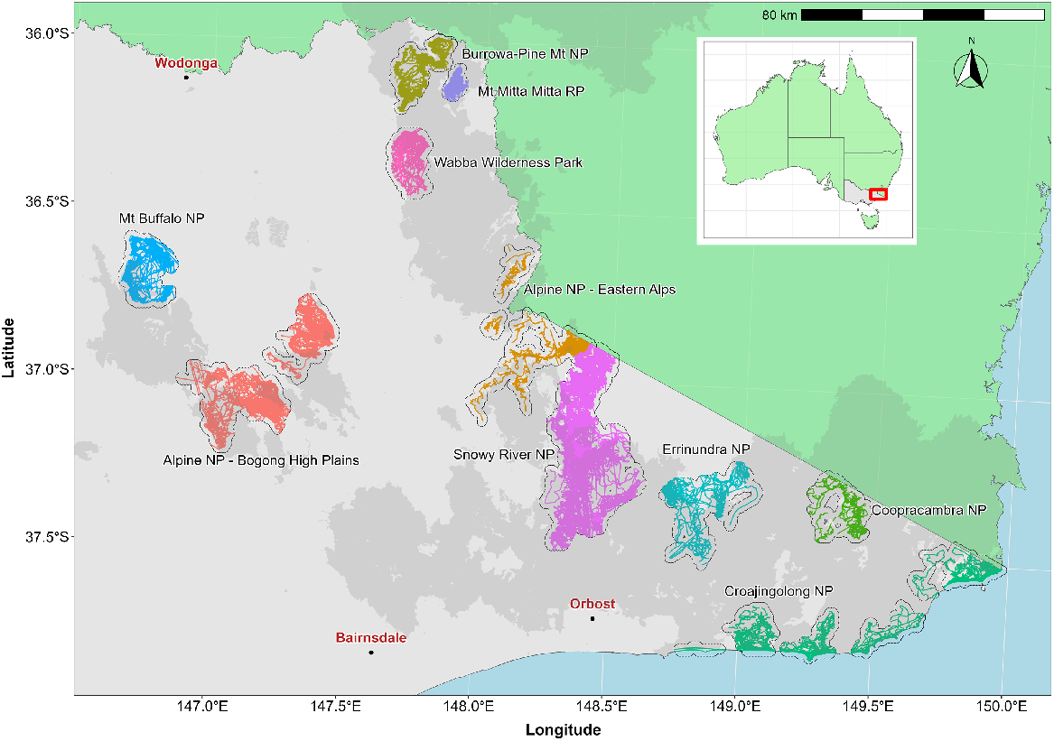
During 2019–20, large-scale, high severity bushfires burnt approximately 1.5 million hectares across Victoria, with the worst affected areas occurring in the North East and East Gippsland regions (Fig. 1). It was estimated that these bushfires affected habitat for around 215 rare or threatened species, with many of these thought to be vulnerable to impacts from invasive species following fire (DELWP 2020). As part of the Victorian Bushfire Biodiversity Response and Recovery program, helicopter-based aerial shooting was implemented as a key threat management activity within priority fire-affected and adjacent public land (DELWP 2021). The objective of the aerial shooting program was to reduce the densities of invasive animals, including sambar deer, fallow deer (Dama dama), feral pigs (Sus scrofa), feral goats (Capra hircus), feral cattle (Bos taurus) and foxes (Vulpes vulpes), within areas of high biodiversity value to assist the survival and recovery of threatened species and ecosystems (DELWP 2021).
Locations of sites where aerial control of invasive animals occurred between February 2020 and May 2022. Coloured lines indicate flight paths flown by the helicopter. Grey polygons surrounding flight paths for each site represent the total operational (search) area. Dark shaded area shows the extent of the 2019–20 bushfires. Inset shows the study area location (red rectangle).
Aerial shooting from a helicopter has been widely used to control deer populations and is considered to be the most effective method for reducing deer abundances over large areas (Forsyth et al. 2013; Latham et al. 2018; Bengsen et al. 2022a). The standard methodology used for measuring the efficacy of control operations is to conduct pre-control monitoring (Bengsen et al. 2022a) or pre- and post-control monitoring with the difference between the indices or population estimates used to infer control efficacy (Forsyth et al. 2013). Alternatively, radio-collars are fitted to deer and their fate monitored with regards to the control method (Latham et al. 2018). These methods of estimating the efficacy of control may incur substantial extra costs due to the necessity of conducting monitoring in addition to the cost of control, especially if ground-based monitoring methods are required.
The shooting of individual animals from a defined area can be viewed as a removal (or depletion) sample, which is a well-known sampling method used to estimate the size of a demographically closed population (DeLury 1947; Zippin 1958; Gould and Pollock 1997). By demographically closed, we mean that the sampled population is closed to additions or losses except those due to the removal method (i.e. no births, deaths, immigration or emigration). The classic removal model was originally developed assuming that removal effort was constant over time (Zippin 1958). However, many applications in fisheries and pest management needed to account for variable removal effort. Thus, modifications of the classic removal model were developed that allowed removal effort to vary over time. These models were termed ‘catch–effort’ models (Schnute 1983; Gould and Pollock 1997; Chao and Chang 1999; St. Clair et al. 2013). Removal methods have a long history in the estimation of animal abundance and have been regularly used to estimate the size of populations exploited by fishing or hunting (Gould and Pollock 1997; Dorazio et al. 2005; Rodriguez de Rivera and McCrea 2021). The advantage of removal or catch–effort models is that they allow estimates of the initial population size to be made directly from the sequence of removals over time. Assuming the population is demographically closed, an estimate of the residual (or post-control) population can be made by simply subtracting the known removals from the estimate of initial population size. This means that estimates of control efficacy can be derived directly from the data collected during control operations, without the need to conduct additional monitoring.
Recent theoretical work has also extended these types of removal models to populations where demographic closure should not be assumed (Dail and Madsen 2011; Link et al. 2018). Here, populations are assumed to be subject to additions or losses between periods of intensive control. Thus, these models include parameters for estimating population growth due to natural recruitment or recolonisation between these intensive control periods (Hostetler and Chandler 2015). Such models are useful when control operations are applied over extended periods where the population could be subject to breeding or immigration from uncontrolled areas.
Here we analyse the aerial shooting operational data collected for sambar deer from 2020 to 2022, conducted at 10 sites located across fire-affected areas of eastern Victoria. Sambar deer were shot from a helicopter and key data recorded as part of the aerial shooting operations, including helicopter flight path (search) data and location data for shot (and killed) animals. We use these data to estimate pre- and post-control densities of sambar deer to assess the effectiveness of the control program at reducing deer abundance. By using models allowing for additions and losses to the population between intensive periods of control, we should gain an understanding of the effect of recruitment and/or recolonisation of individuals into an area following control and its subsequent effect on the estimates of control efficacy. The model was also used to inform management by recommending the intensity of future control effort required to achieve target reductions in abundance.
Methods
Study area
Aerial shooting of introduced animals (deer, feral pigs, feral goats, feral cattle and foxes) in the North East and East Gippsland regions of Victoria occurred across seven national parks (NP; Alpine, Mt Buffalo, Burrowa-Pine Mountain, Croajingolong, Coopracambra, Errinundra and Snowy River), as well as Mt Mitta Mitta Regional Park (RP) and the Wabba Wilderness Park (WP) (Fig. 1). Due to the size of the Alpine National Park, aerial shooting was focused within two separate areas, the Bogong High Plains and the Eastern Alps. Thus, 10 sites were the subject of aerial shooting (Fig. 1). The topography and vegetation across the study area was variable but generally mountainous and dominated by montane forest, especially alpine ash (Eucalyptus delegatensis) and mountain ash (E. regnans) on mountain slopes, with a range of eucalypt species dominating at lower altitudes (e.g. E. sieberi, E. globoidea, E. cypellocarpa, E obliqua). Coastal areas comprised mainly shrubby dry forest, riparian scrub and Banksia (Banksia serrata) woodland (https://www.environment.vic.gov.au/biodiversity/bioregions-and-evc-benchmarks). Elevation ranged from around 1820 m (Mt Cope – Alpine NP) to near sea level (coastal areas – Croajingolong NP). Rainfall in the region was variable, with annual totals averaging more than 1800 mm in alpine areas to 890 mm at lower altitudes (Australian Bureau of Meteorology; http://www.bom.gov.au). The impact of the 2019–20 bushfires within each of the 10 sites was variable, with around 90% of the forest canopy burnt in the Burrowa-Pine Mountain NP compared with only 18% in the Alpine NP – Eastern Alps.
Aerial operations
Aerial shooting operations were conducted in accordance with all relevant Victorian interagency aviation operating procedures, including SO 4.06 Aerial shooting operations (Victorian Government 2020) and the Parks Victoria Aerial Shooting Guideline (Parks Victoria 2020). Aerial shooting was conducted from a helicopter (AS350 B2 Squirrel, Airbus Helicopters, Marignane, France) with the pilot in the front right seat, one shooter in the rear right seat and one spotter in the front left seat, whose primary role was acting as an air safety observer, but who also relayed sightings of deer to the shooter and recorded data. Aerial shooting procedures placed an emphasis on the humane destruction of animals in accordance with Victorian animal welfare legislation (Victorian Government 1986). The shooter used a semi-automatic centre fire rifle (.308 calibre) firing protected point ammunition ranging from 130 to 180 grains, suitable for use on large herbivores. Only shots to the thorax (heart-lung) or head were taken under favourable conditions. This was followed up with further heart-lung shots once the animal had collapsed to ensure a rapid death. The pilot was required to verbally confirm the death of the animal, with assistance of the observer and shooter, prior to continuing the search. Independent on-ground veterinarian audits were conducted over the course of the operation to ensure procedural compliance (e.g. verify shot placement and the use of multiple shots per animal). The destruction of wild deer as part of the operations were authorised under an Authority to Control Wildlife permit issued by the Victorian Office of the Conservation Regulator in consultation with the Game Management Authority.
Operational data
Aerial shooting at each site was undertaken between February 2020 and May 2022. Aerial shooting effort was grouped into five distinct periods representing times when intensive control occurred. However, not all sites were subject to control during each period (Table 1). Operational data consisted of spatial layers representing locations of all shot and killed animals (‘removals’), as well as records of animals observed where a shot was not taken. However, the latter were not used in the present analysis because animals observed may have been shot at a later occasion. Additional spatial data were also available for the routes flown by the helicopter while actively undertaking control (‘search effort’) as well as aerial mission (flight) dates. For each site, the total search area was defined by discretising the continuous search route by overlaying a 1-km grid on to the helicopter flight paths, aggregated over all periods. The total operational area (=total search area) for each site used in subsequent analyses (e.g. deer density estimates) was then defined as the area of the combined grids cells (Fig. 1).
| Site | February–May 2020 | June–October 2020 | March–May 2021 | September–December 2021 | March–May 2022 |
|---|---|---|---|---|---|
| Alpine NP – Bogong | 373 (70) | 1734 (310) | 1311 (188) | 1393 (122) | 2571 (328) |
| Alpine NP – Eastern | 699 (95) | 0 (0) | 183 (14) | 602 (45) | 379 (37) |
| Burrowa NP | 537 (12) | 674 (42) | 112 (3) | 819 (47) | 157 (2) |
| Coopracambra NP | 57 (1) | 195 (1) | 129 (0) | 147 (5) | 88 (0) |
| Croajingolong NP | 893 (37) | 591 (27) | 666 (38) | 167 (3) | 499 (44) |
| Errinundra NP | 159 (3) | 435 (20) | 437 (19) | 244 (21) | 191 (14) |
| Mt Buffalo NP | 281 (63) | 804 (118) | 2020 (113) | 696 (63) | 1643 (222) |
| Mt Mitta Mitta RP | 223 (7) | 211 (13) | 92 (4) | 186 (7) | 82 (0) |
| Snowy River NP | 3811 (1105) | 6632 (1247) | 3374 (382) | 3550 (395) | 1424 (184) |
| Wabba WP | 520 (32) | 309 (37) | 0 (0) | 1250 (173) | 163 (29) |
| Totals | 7553 (1425) | 11 585 (1815) | 8324 (761) | 9054 (881) | 7197 (860) |
NP, national park; RP, regional park; WP, wilderness park.
The data on sambar deer removed and search effort expended per unit time (‘catch and effort data’) can be used to estimate the size of the initial sambar deer population within the operational area at each site, as well as the rate of detection (and removal) per unit of search effort (Gould and Pollock 1997; Chao and Chang 1999). To facilitate analysis, data from individual helicopter missions within each of the five periods of control were aggregated into five removal occasions. Thus, we adopted a robust design for the data with five primary periods, with each primary period consisting of five occasions (secondary periods). As the length of each period was roughly 4 months, each occasion corresponded to roughly 24 days and could consist of several missions. This was undertaken to ensure that search coverage was consistent between occasions. Because missions were staggered among sites, some sites had no mission data for one or more occasions, with some sites having no mission data for a particular period. These missing data windows were treated as missing completely at random and accounted for in the analysis.
Analysis of the sequence of removals and search effort for each occasion within each period were used to estimate the initial site abundance (i.e. before the start of removal activities) and the detection rate per unit of search effort. Using the estimate of initial abundance at the start of the period, the residual site abundance following the final removal occasion () could also be derived. Because there were five distinct periods of control spanning 27 months, it would be unreasonable to assume that the population at each site was demographically closed (i.e. no additions or losses to the population other than removals) over this entire control period. For example, sambar deer births occur all year round, with a peak between April and July (Watter et al. 2020), so the operational data encompasses at least two entire breeding seasons. Movement of deer in response to increasing snow depth at higher altitudes is also likely to have occurred during this period (Comte et al. 2022). To account for these potential demographic changes over the entire control period, we assumed that populations at each site were open to demographic changes between each of the five control periods and closed to demographic changes within each period. A summary of the aerial shooting data undertaken at each site during each period is given in Table 1.
To account for demographic changes to the population (other than removals), a generalised N-mixture model was employed (Dail and Madsen 2011; Hostetler and Chandler 2015). The generalised N-mixture model explicitly models change in the population between sampling periods, allowing the closure assumption underpinning the standard N-mixture model to be relaxed. By modelling population change as a function of parameters governing ‘additions’ or ‘losses’ between sampling periods, as well as imperfect detection, unbiased estimates of population abundance are possible using counts from ‘open’ populations (Dail and Madsen 2011; Hostetler and Chandler 2015). The structure of the generalised N-mixture model used to analyse the removal and search effort data for each site and period is described further below.
Generalised N-mixture model
The generalised N-mixture model used here assumed that removals followed a multinomial observation process over occasions within each period (Dorazio et al. 2005; Haines 2020). Separately for each of the five periods, the number of individuals that were removed from each site were divided into five occasions, and individuals were assigned to an occasion based on the date it was shot.
The counts of individuals shot within a particular site i, (i = 1,…,I) during a particular period t, (t = 1,…,T) and occasion j, (j = 1,…,J) (yijt) therefore represented a multinomial sample y ~ Multinomial(n, π) with cell probabilities for each occasion j(πj) equal to:
where pj was the probability of detection (and removal) during occasion j and n was the total number of individuals removed from the operational area, during that period.
It follows that the total number of individuals removed during the period was dependent on the total population size at the start of the period (i.e. j = 0) and the probability of removal over all occasions. The latter was calculated as:
and the complete model for the total abundance for each site i and period t(Nit), allowing for demographic changes between periods, was given by:
where the conditional cell probabilities . The intercepts βi represented the average (baseline) initial abundance at each site i (i.e. before the start of control activities), and Rit was the residual abundance at the end of the period, which was given simply by subtracting the number removed during the period from the abundance at the start of the period.
The parameter was fitted to the model as an offset representing the (log) search area (km2) subject to aerial control. The parameter rit represents the per-capita rate of increase in the population at site i between periods t − 1 and t, with r > 0 representing an increase and r < 0 representing a decrease. The rit were modelled as a linear function of the average elevation (metres above sea level; m.a.s.l.) of site i (Ai) and season (winter/summer) occurring between period t − 1 and t(St), with η1,…,4 being parameters to be estimated. To facilitate estimation, values for the average elevation for each site were standardised by subtracting the mean and dividing by the standard deviation.
The detection (and removal) probability pijt was modelled as a linear function (on the complementary log-log scale) of the amount of helicopter search effort (km) Eijt, with α0 representing the (log) removal rate for one unit of search effort (i.e. hazard rate). We also allowed the detection probability to vary over occasions by adopting a model for the baseline hazard rate (Allison 1982). This was achieved by allowing the detection probability to depend on occasion j according to parameter κi, which allowed the detection probability to also vary for each site i. Values of κ less than zero indicated that the detection probability decreased with increasing occasions, while values less than zero indicated a corresponding increase with occasion number. A hierarchical normal prior distribution was used to model κi, with mean μk and standard deviation σk.
To account for the differing sizes of each site, Eijt was also standardised by dividing by the size of the operational search area at each site (in km2). Thus, units of effort were effectively km of search effort per km2 of total habitat searched. Finally, an estimate of the overall percentage decline in the population achieved over the five periods was given by:
which was calculated by taking the ratio of the residual abundance in the last period (Period 5) to the initial abundance in the first period (Period 1) for each site i. Similar metrics were also calculated separately for each period in each site (e.g. ).
The model specified in Eqns 1, 2 was fitted to the joint removal data for sambar deer from all 10 sites in a Bayesian framework by Markov chain Monte Carlo (MCMC) using Nimble (NIMBLE Development Team 2022). Weakly informative normal or half-normal priors, specified as N(0, 5), were specified for all unknown parameters. We judged convergence of the posterior distribution of the parameters based on visual inspection of traceplots and estimates of the Brooks–Gelman–Rubin convergence criterion from three independent chains (Brooks and Gelman 1998). Following convergence, the model was updated for 10 000 iterations, leaving a total of 30 000 samples for each parameter, which were used for further inference. We assessed model fit by conducting posterior predictive checks (Gelman et al. 1996), which involved comparing the number of removals in each area during each period with the corresponding number predicted by the model
One of the assumptions underlying the use of the removal model in Eqns 1, 2 is that animals removed at each occasion and period are a representative sample of the population (Dorazio et al. 2005). This assumption may be violated to some degree if the area at a site is searched sequentially rather than repeatedly. We examined the extent to which the operational area at each site was subject to repeated search by examining the area searched during each period as a proportion of the total operational area. This was calculated by summing the number of 1-km grid cells searched each period and dividing by the total number of 1-km grid cells constituting the operational area.
Search effort recommendations
The parameter estimates from the fitted model in Eqns 1, 2 included an estimate of the removal probability per km of helicopter search effort (parameter α0). This parameter can be used, in turn, to estimate the amount of search effort that would be required to achieve a certain level of population reduction. Accordingly, posterior estimates of α0 and κi were used in a Monte Carlo simulation approach to examine the intensity of helicopter search effort required to reduce population abundances of sambar deer by various proportional amounts. Simulated search effort was divided into several removal occasions to replicate operational conditions where consecutive ‘missions’ are usually conducted in a particular site over several months. However, we limited this approach to occur within a single period, where the population was assumed to be closed to natural additions or losses.
Given an initial abundance within a notional site i, simulated removal of individuals occurred over each removal occasion j, with the probability of removal calculated as
where Pj is the probability of removal during occasion j(j = 1,…,J), given search effort Ej (km per km2 of habitat) and parameters α0 and κi were estimated by Eqn 2. The number of occasions (J) was set at 5 and the initial abundance was set to the mean initial abundance estimated from the 10 sites. The predicted search effort required to achieve various levels of population reduction was compared with that achieved from each site, in each of the five periods, by overlaying the estimated population reductions and associated actual search effort onto the plots of predicted search effort.
Results
The total number of sambar deer shot through aerial shooting operations across the 10 sites over the five periods (February 2020–May 2022) was 5742 (Table 1). The majority of these were in the Snowy River NP (3313), with the next highest removals in the Alpine NP – Bogong High Plains (1018). Over 43 650 km of helicopter search effort was undertaken in these 10 sites over the same period, with the most effort expended in the Snowy River NP (Table 1). Average search effort per mission was 154 km, and 80% of missions were between 48 and 232 km.
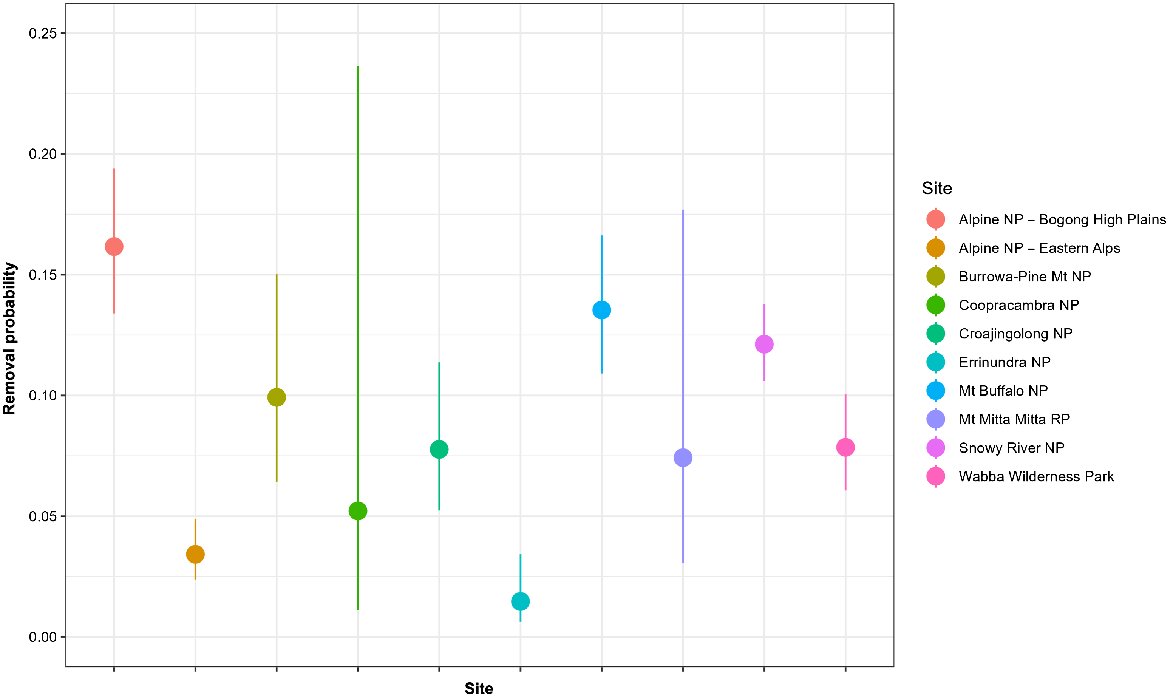
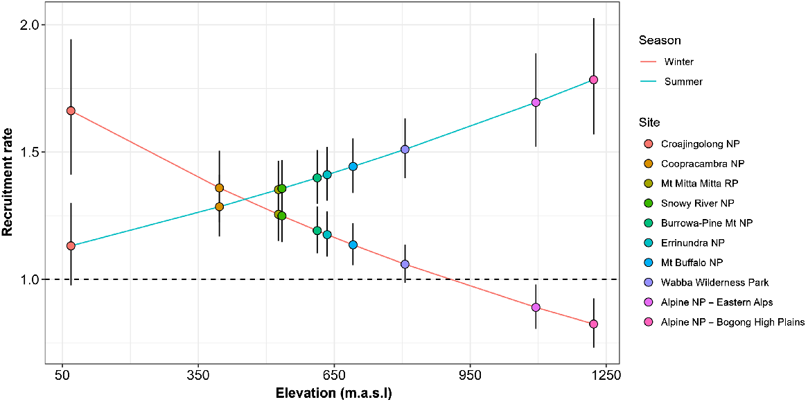
Fitting of the generalised N-mixture model (Eqns 1, 2) to the joint removal data from the 10 sites was judged to have converged after 100 000 iterations, based on visual inspections of the traceplots and values for < 1.01 (Supplementary Table S1). The model also appeared to provide an adequate fit to the data, as judged by the posterior predictive checks of the total number of deer removed compared with that predicted by the model (Fig. S1). Estimates of the detection (and removal) rate of individual sambar deer suggested that the average probability of detecting individuals from the helicopter was 0.11 (95% CI: 0.09, 0.12) per km of search effort, per km2 of habitat. However, the detection probability varied among sites, being highest in the Alpine NP – Bogong High Plains at 0.15 per km of search effort per km2 of habitat, and lowest at Errinundra NP at 0.02 per km of search effort per km2 of habitat (Figs 2, S2). Apart from removals, the rate of natural recruitment (r) of sambar deer also varied with the elevation (m.a.s.l.) of each site as well as season (winter or summer). Populations of sambar deer in operational areas at the highest elevations (e.g. Alpine NP) exhibited decreases over the winter period and large increases over the summer period (Fig. 3). Conversely, populations in operational areas at the lowest elevations (e.g. Croajingolong NP) exhibited the highest increases during the winter period and the lowest during the summer period (Fig. 3). The recruitment rates in other operational areas were intermediate between these two extremes (Fig. 3).
The probability of detection and removal of sambar deer for each site during the final occasion for a helicopter search effort of 1 km searched per km2 of habitat. Error bars are 90% credible intervals. NP, national park; RP, regional park; WP, wilderness park.
Relationship between the recruitment rate (er) of sambar deer due to natural additions and losses between periods and elevation (metres above sea level; m.a.s.l.) and season (summer/winter). Values greater than 1.0 indicate net population increases; values less than 1.0 indicate net decreases. Points represent the estimates for each site with colours in ascending order of elevation. Error bars are 90% credible intervals. NP, national park; RP regional park.
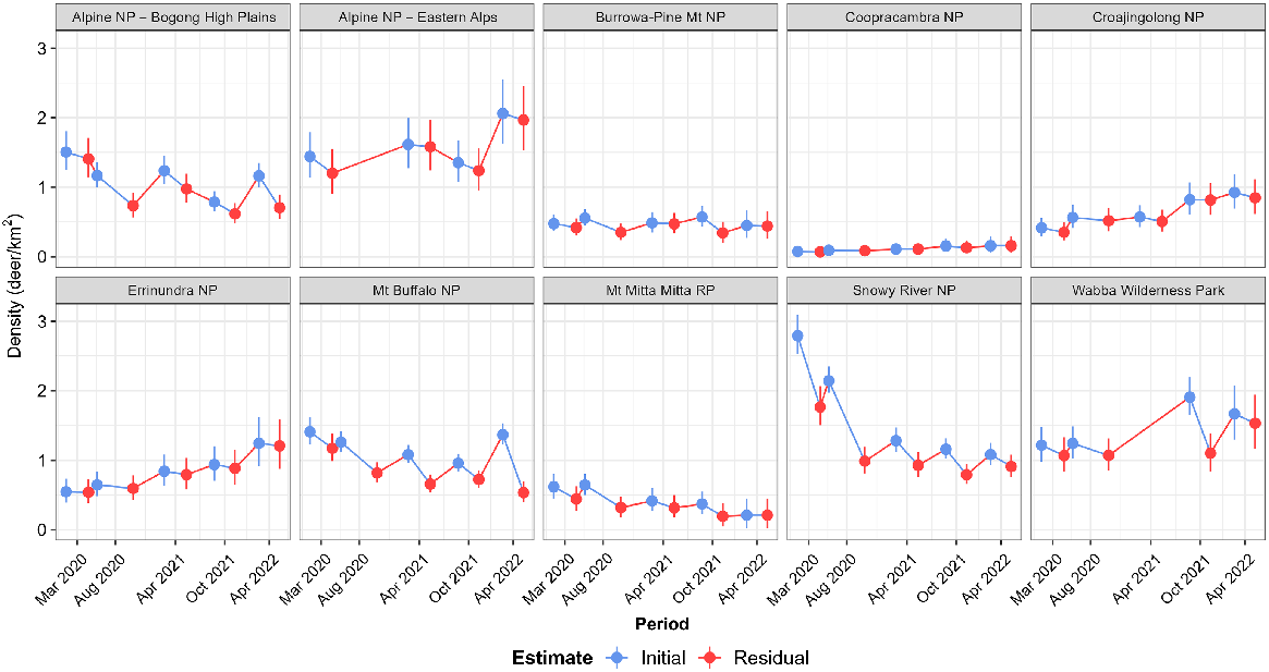
The estimated initial () and residual () abundance of sambar deer at each site resulted in the highest population reductions over the five periods (Eqn 3) in the Snowy River NP and Mt Mitta Mitta RP, at 68% and 66%, respectively (Fig. 4, Table 2). Population reductions of 62% and 53% were also obtained at the Mt Buffalo NP and Alpine NP – Bogong High Plains sites. Reductions at Burrowa-Pine Mountain NP, Wabba WP and Coopracambra NP were uncertain, and populations increased at the remaining operational areas (Fig. 4, Tables 2, S2).
Estimates of the initial ( – blue points) and residual ( – red points) densities of sambar deer for each period of aerial control at 10 sites in Eastern Victoria. Vertical lines indicate the 90% credible intervals for the estimates. NP, national park; RP, regional park.
| Site | Decline (%) | LCI | UCI |
|---|---|---|---|
| Snowy River NP | 68 | 64 | 71 |
| Mt Mitta Mitta RP | 66 | 29 | 94 |
| Mt Buffalo NP | 62 | 52 | 71 |
| Alpine NP – Bogong High Plains | 53 | 45 | 61 |
| Burrowa-Pine Mountain NP | 8 | −29 | 40 |
| Wabba WP | −27 | −57 | 1 |
| Alpine NP – Eastern Alps | −37 | −67 | −11 |
| Croajingolong NP | −108 | −171 | −55 |
| Errinundra NP | −124 | −187 | −70 |
| Coopracambra NP | −126 | −313 | 5 |
Negative values indicate population increases.
LCI, lower 90% credible limit; UCI, upper 90% credible limit.
Proportion of the operational area at a site covered during every period varied among sites, from an average of 34% at the Alpine NP – Eastern Alps to 95% at Mt Mitta Mitta RP (Table S3).
Search effort recommendations
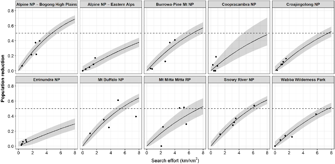
The reductions achieved during each period of aerial control varied widely among sites and was dependent on the amount of search effort conducted (Fig. 5). The highest reduction during a single period occurred at Mt Buffalo NP during period 5 (March–May 2022), which reduced the abundance of sambar deer by 61% and required 5 km of search effort per km2 of habitat (Fig. 5). Similarly high (>50%) reductions were achieved in the Snowy River NP and Mt Mitta Mitta RP during period 2 (June–October 2020), and again at Mt Mitta Mitta RP during period 4 (September–December 2021) (Fig. 5).
The proportional reduction in population density of sambar deer estimated for each of the five periods for each site, plotted against the actual amount of search effort undertaken (solid points). Solid line is the relationship between the proportional reduction and increasing search effort predicted for each site (Eqn 4). Shaded area is the 90% credible intervals. Horizontal dashed line indicates a 50% reduction. Search effort is total helicopter search effort expended during the period. NP, national park; RP, regional park.
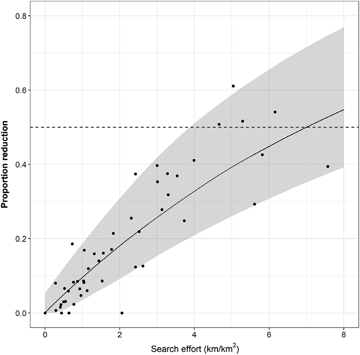
More generally, the amount of search effort predicted to be required to achieve various levels of proportional reductions in sambar deer densities (Eqn 4) over a single period suggested that a 50% reduction in density could be achieved with 7 km of search effort per km2 of habitat (Fig. 6). This equates to 1.4 km/km2 of effort in each of five removal occasions. Simulated reductions in sambar deer densities and associated 90% credible intervals encompassed the majority of the actual reductions achieved at each site over the five periods, suggesting that the simulated relationship was a good match for the estimated reductions (Fig. 6).
Relationship between the proportional reduction in sambar deer density and increasing search effort predicted from the combined data from each site (Eqn 4). Shaded area is the 90% credible interval. Points are the estimated reductions achieved in each site for each period against the actual amount of search effort undertaken in each period. Horizontal dashed line indicates a 50% reduction.
Discussion
The analyses presented here used standard operational data collected during an extensive and intensive aerial shooting program to reduce introduced animal abundance in eastern Victoria. During this program, the collection of location data for all shot (and killed) deer, as well as the recording of concurrent search effort data (helicopter search paths), allowed initial abundance, detectability (removal rate) and proportion of the population removed to be estimated using models based on ‘removal’ (or ‘catch–effort’) sampling (Gould and Pollock 1997; Dorazio et al. 2005; Haines 2020). Estimates of these parameters were obtained for sambar deer removal from 10 sites. Initial densities of sambar deer estimated by the removal model ranged from 0.1 to 2.8 deer/km2 (mean 1 deer/km2). These were similar to those estimated recently for sambar deer from similar forest types in nearby Kosciuszko NP using spatial capture–recapture methods (mean 1.6 deer/km2) (Bengsen et al. 2022b). An important aspect of the catch–effort model used here was the ability to relax the assumption of demographic closure, allowing an estimation of additions and losses between periods of intensive control. Population growth between periods of control was shown to be strongly related to elevation and season, which had implications for the recovery of sambar deer populations from aerial shooting among the different sites.
Analysis of the aerial shooting data suggested that sambar deer abundance was reduced by around 50–70% at sites where aerial search effort was high (i.e. >3 km/km2) for most periods. However, results at the remaining sites suggest that sambar deer densities have either remained static or increased over the five periods of aerial control. There were two main reasons for the variation in efficacy of the aerial shooting program among the different sites. The first reason was that the level of population reduction achieved was strongly related to the amount of aerial search effort per unit area, a result also found by Bengsen et al. (2022a). Deer populations in sites that exhibited no change or increases in deer densities inevitably were subject to relatively low helicopter search effort per km2 of habitat (e.g. Coopracambra NP, Errinundra NP) compared with sites that exhibited decreases in sambar deer densities (e.g. Snowy River NP, Mt Mitta Mitta RP). The second reason was that there was variation in the recruitment rates of sambar deer among different sites, which was dependent on both season and elevation, with areas at the highest elevations (Alpine NP – Bogong High Plains and Eastern Alps) exhibiting a net decrease in abundance during winter followed by net increases during summer. This pattern was reversed for areas at low elevation (e.g. Croajingolong NP), where recruitment was highest during winter and lowest during summer. Other studies have shown that sambar deer move to lower elevations when snow cover increases at high elevations (Comte et al. 2022). The seasonal variation in recruitment among sites estimated here would appear to support this phenomenon, and suggests that recruitment during our study was driven largely by seasonal movement of sambar deer.
Sambar deer recruitment at some sites (e.g. Errinundra NP, Croajingolong NP, Alpine NP – Eastern Alps) was sufficient to offset reductions due to aerial shooting, resulting in increases in sambar deer densities over the duration of the study. Increased recruitment of deer may be related to the recovery of vegetation in these areas post-fire, especially in areas heavily burnt during 2019–20 (e.g. Errinundra NP, Croajingolong NP). Deer have been shown to re-occupy areas recovering from bushfires within 18–24 months post fire (Forsyth et al. 2012); the abundances of sambar deer in areas heavily burnt during the 2019–20 bushfires may have been depleted initially when aerial control commenced, with populations now increasing as the understorey vegetation recovers in these areas. These areas were also ones that received relatively lower aerial control effort, which was more concentrated at those sites with higher initial densities of deer. As the deer population recovers in those areas heavily burnt by the 2019–20 bushfires, their priority for future aerial control effort should also increase to limit the potential recovery of deer populations in these areas.
Aerial control efficiencies differed among locations, being relatively high in some areas such as the Alpine NP – Bogong High Plains, Mt Buffalo NP, Burrowa-Pine Mt NP and the Snowy River NP, and relatively low in other areas such as the Alpine NP – Eastern Alps, Errinundra NP and Coopracambra NP. In general, reductions in Sambar deer densities of 50% could be achieved over a single period of intensive control with 7 km of search effort per km2 of habitat. For areas with relatively high control efficiencies, this could be reduced to 5 km/km2 of search effort. In practice, the recommended search effort for a single period would need to be undertaken over several occasions, defined as the number of helicopter missions required to undertake at least one complete search of the operational area. Thus, five occasions would be equivalent to at least five complete searches of the operational area, with each occasion consisting of 1.4 km/km2 of search effort (i.e. 7 km/km2 total).
Despite a long history of animal abundance estimation, especially in fisheries management (DeLury 1947; Schnute 1983; Mäntyniemi et al. 2005), there are few examples of the use of catch–effort models on data collected during aerial shooting operations (Ramsey et al. 2009; Davis et al. 2016b, 2018). Studies applying catch–effort models to feral pig removal in the USA found that aerial shooting removed between 47% and 67% of feral pigs following three removal occasions (Davis et al. 2016b, 2018). Similarly, an analysis of the removal of feral pigs from Santa Cruz Island, California showed that around 77% of the total population of pigs were removed by aerial shooting (Parkes et al. 2010). A recent study of the efficacy of aerial shooting for removing deer from agricultural areas in NSW and Qld found that shooting from a helicopter achieved reductions in deer densities ranging from 5% to 75% for fallow deer and 48–88% for chital deer (Bengsen et al. 2022a).
In Australia, aerial shooting has been used to reduce the abundance of introduced animals such as deer (Bengsen et al. 2022a), feral pigs (Choquenot et al. 1999), dromedary camels (Camelus dromedarius) (Hampton et al. 2016), donkeys (Equus asinus) (Wheeler 1984) and feral goats (Capra hircus) (Pople et al. 1998). However, none of these studies attempted to use the operational data to estimate population abundance. Rather, the efficacy of aerial shooting was evaluated by conducting additional monitoring either before or both before and after the aerial shooting operation (Pople et al. 1998; Choquenot et al. 1999). This could add a considerable additional expense to the control program, especially if ground-monitoring methods are required. In contrast, the analyses presented here offer an alternative method for measuring the efficacy of aerial animal control operations that does not rely on the collection of additional monitoring data. However, one advantage of conducting additional monitoring is that the estimates of animal abundance are obtained in advance of applying control, and can then be used to aid the operational planning of resources (Bengsen et al. 2022a). This is not possible with the present approach, which requires collection of the control data first to estimate population abundance.
A disadvantage of catch–effort models is that not all aerial shooting operational data may be suitable for estimating population abundance. For valid and precise estimates to be obtained from catch–effort data, the removal method must be able to remove individuals at a rate faster than they can be replaced, either by reproduction or immigration. However, by jointly analysing data from 10 sites in the current analyses, reasonable estimates were still able to be obtained for sites with sparse removal data. Another assumption of the catch–effort model used here is that successive removals should be representative of the total population. This could be violated if search effort occurs sequentially across the area of interest rather than as repeated searches of the same area. Analysis of the coverage of the total search area achieved during each of the control periods ranged from 34% to 95%, indicating the proportion of the total search area that was subject to repeat searching, across the five periods. The implications of some sequential coverage of the area of interest on estimates from catch–effort models remains unknown, but would be a worthy topic for future investigation.
The analysis of aerial search effort required has suggested the amount of search effort needed to effect various proportional reductions of sambar deer. These estimates can be used by management agencies to plan future deer control operations and estimate likely costs to achieve target densities. This was undertaken in the recent study by Bengsen et al. (2022a) using hours of operation as the metric of search effort. Most studies of aerial shooting operations have quantified effort in terms of the number of hours of aerial operation rather than the distance travelled, as was used here. It is likely that both distance and time spent searching would be highly correlated and whether one is better than the other for quantifying search effort should be the subject of future investigation.
Finally, how much reduction in deer densities is required to protect biodiversity assets remains a point of conjecture. Studies using exclosures to measure deer impacts have provided evidence that deer reduce vegetation cover and inhibit tree regeneration and sapling growth (Forsyth et al. 2015a; Davis et al. 2016a). In Victoria, the relationships between deer densities and deer impacts have only recently been investigated (Bennett et al. 2022), and additional studies are likely to be required to set appropriate management targets for deer control.
Data availability
The data and code used to undertake the analyses in this study will be made available at Zenodo (https://doi.org/10.5281/zenodo.7302401).
Declaration of funding
The aerial shooting program was established and supported through the Victorian Government’s funding package to support the Bushfire Biodiversity Response and Recovery program. Additional funding was also provided through the Australian Government’s Regional Fund for Wildlife and Habitat Bushfire Recovery.
Acknowledgements
Parks Victoria led the operational delivery of the aerial shooting program from June 2020 – particularly, Sandra Robinson, Brooke Ryan, Iris Curran, Darren Baldyga and Deirdre Griepsma. Many thanks to the aerial shooting contractors and all the Parks Victoria and Department of Environment Land, Water and Planning (DELWP) staff involved in the operational delivery or providing regional on-ground support. We thank Kaustuv Dahal for the mapping and collating of spatial data on deer removal locations and flight paths of the helicopter to enable the analyses undertaken here. This manuscript was improved by constructive comments from Dave Forsyth, Peter Caley and two anonymous reviewers.
References
Allison PD (1982) Discrete-time methods for the analysis of event histories. Sociological Methodology 13, 61-98.
| Crossref | Google Scholar |
Barrette M, Bélanger L, De Grandpré L, Ruel J-C (2014) Cumulative effects of chronic deer browsing and clear-cutting on regeneration processes in second-growth white spruce stands. Forest Ecology and Management 329, 69-78.
| Crossref | Google Scholar |
Bengsen AJ, Forsyth DM, Pople A, Brennan M, Amos M, Leeson M, Cox TE, Gray B, Orgill O, Hampton JO, Crittle T, Haebich K (2022a) Effectiveness and costs of helicopter-based shooting of deer. Wildife Research
| Crossref | Google Scholar |
Bengsen AJ, Forsyth DM, Ramsey DSL, Amos M, Brennan M, Pople AR, Comte S, Crittle T (2022b) Estimating deer density and abundance using spatial mark–resight models with camera trap data. Journal of Mammalogy 103, 711-722.
| Crossref | Google Scholar |
Bennett A, Fedrigo M, Greet J (2022) A field method for rapidly assessing deer density and impacts in forested ecosystems. Ecological Management & Restoration 23, 81-88.
| Crossref | Google Scholar |
Brooks S, Gelman A (1998) General methods for monitoring convergence of iterative simulations. Journal of Computational and Graphical Statistics 7, 434-455.
| Crossref | Google Scholar |
Chao A, Chang S-H (1999) An estimating function approach to the inference of catch–effort models. Environmental and Ecological Statistics 6, 313-334.
| Crossref | Google Scholar |
Choquenot D, Hone J, Saunders G (1999) Using aspects of predator–prey theory to evaluate helicopter shooting for feral pig control. Wildlife Research 26, 251-261.
| Crossref | Google Scholar |
Comte S, Thomas E, Bengsen AJ, Bennett A, Davis NE, Freney S, Jackson SM, White M, Forsyth DM, Brown D (2022) Seasonal and daily activity of non-native sambar deer in and around high-elevation peatlands, south-eastern Australia. Wildlife Research 659-672.
| Crossref | Google Scholar |
Côté SD, Rooney TP, Tremblay J-P, Dussault C, Waller DM (2004) Ecological impacts of deer overabundance. Annual Review of Ecology, Evolution, and Systematics 35, 113-147.
| Crossref | Google Scholar |
Dail D, Madsen L (2011) Models for estimating abundance from repeated counts of an open metapopulation. Biometrics 67, 577-587.
| Crossref | Google Scholar |
Davis NE, Bennett A, Forsyth DM, Bowman DMJS, Lefroy EC, Wood SW, Woolnough AP, West P, Hampton JO, Johnson CN (2016a) A systematic review of the impacts and management of introduced deer (family Cervidae) in Australia. Wildlife Research 43, 515.
| Crossref | Google Scholar |
Davis AJ, Hooten MB, Miller RS, Farnsworth ML, Lewis J, Moxcey M, Pepin KM (2016b) Inferring invasive species abundance using removal data from management actions. Ecological Applications 26, 2339-2346.
| Crossref | Google Scholar |
Davis AJ, Leland B, Bodenchuk M, VerCauteren KC, Pepin KM (2018) Costs and effectiveness of damage management of an overabundant species (Sus scrofa) using aerial gunning. Wildlife Research 45, 696.
| Crossref | Google Scholar |
DeLury DB (1947) On the estimation of biological populations. Biometrics 3, 145-167.
| Crossref | Google Scholar |
Dorazio RM, Jelks HL, Jordan F (2005) Improving removal-based estimates of abundance by sampling a population of spatially distinct subpopulations. Biometrics 61, 1093-1101.
| Crossref | Google Scholar |
Forsyth DM, Gormley AM, Woodford L, Fitzgerald T (2012) Effects of large-scale high-severity fire on occupancy and abundances of an invasive large mammal in south-eastern Australia. Wildlife Research 39, 555-564.
| Crossref | Google Scholar |
Forsyth DM, Ramsey DSL, Veltman CJ, Allen RB, Allen WJ, Barker RJ, Jacobson CL, Nicol SJ, Richardson SJ, Todd CR (2013) When deer must die: large uncertainty surrounds changes in deer abundance achieved by helicopter- and ground-based hunting in New Zealand forests. Wildlife Research 40, 447-458.
| Crossref | Google Scholar |
Forsyth DM, Wilson DJ, Easdale TA, Kunstler G, Canham CD, Ruscoe WA, Wright EF, Murphy L, Gormley AM, Gaxiola A, Coomes DA (2015a) Century-scale effects of invasive deer and rodents on the dynamics of forests growing on soils of contrasting fertility. Ecological Monographs 85, 157-180.
| Crossref | Google Scholar |
Forsyth DM, Stamation K, Woodford L (2015b) Distributions of sambar deer, rusa deer and sika deer in Victoria. Unpublished client report for the Biosecurity Branch, Department of Economic Development, Jobs, Transport and Resources. Arthur Rylah Institute for Environmental Research, Victorian Department of Environment, Land, Water and Planning, Melbourne, Vic., Australia.
Gelman A, Meng XL, Stern H (1996) Posterior predictive assessment of model fitness via realized discrepancies. Statistica Sinica 6, 733-807.
| Google Scholar |
Gould WR, Pollock KH (1997) Catch-effort maximum likelihood estimation of important population parameters. Canadian Journal of Fisheries and Aquatic Sciences 54, 890-897.
| Crossref | Google Scholar |
Haines LM (2020) Multinomial N-mixture models for removal sampling. Biometrics 76, 540-548.
| Crossref | Google Scholar |
Hampton JO, Jones B, Perry AL, Miller CJ, Hart Q (2016) Integrating animal welfare into wild herbivore management: lessons from the Australian Feral Camel Management Project. The Rangeland Journal 38, 163-171.
| Crossref | Google Scholar |
Hostetler JA, Chandler RB (2015) Improved state–space models for inference about spatial and temporal variation in abundance from count data. Ecology 96, 1713-1723.
| Crossref | Google Scholar |
Latham ADM, Cecilia Latham M, Herries D, Barron M, Cruz J, Anderson DP (2018) Assessing the efficacy of aerial culling of introduced wild deer in New Zealand with analytical decomposition of predation risk. Biological Invasions 20, 251-266.
| Crossref | Google Scholar |
Link WA, Converse SJ, Yackel Adams AA, Hostetter NJ (2018) Analysis of population change and movement using robust design removal data. Journal of Agricultural, Biological and Environmental Statistics 23, 463-477.
| Crossref | Google Scholar |
Mäntyniemi S, Romakkaniemi A, Arjas E (2005) Bayesian removal estimation of a population size under unequal catchability. Canadian Journal of Fisheries and Aquatic Sciences 62, 291-300.
| Crossref | Google Scholar |
NIMBLE Development Team (2022) NIMBLE: MCMC, particle filtering, and programmable hierarchical modeling. R package version 0.13.1. Available at https://cran.r-project.org/package=nimble
Parkes JP, Ramsey DSL, Macdonald N, Walker K, McKnight S, Cohen BS, Morrison SA (2010) Rapid eradication of feral pigs (Sus scrofa) from Santa Cruz Island, California. Biological Conservation 143, 634-641.
| Crossref | Google Scholar |
Pople AR, Clancy TF, Thompson JA, Boyd-Law S (1998) Aerial survey methodology and the cost of control for feral goats in Western Queensland. Wildlife Research 25, 393-407.
| Crossref | Google Scholar |
Ramsey DSL, Parkes J, Morrison SA (2009) Quantifying eradication success: the removal of feral pigs from Santa Cruz Island, California. Conservation Biology 23, 449-459.
| Crossref | Google Scholar |
Rodriguez de Rivera O, McCrea R (2021) Removal modelling in ecology: a systematic review. PLoS ONE 16, e0229965.
| Crossref | Google Scholar |
Schnute J (1983) A new approach to estimating populations by the removal method. Canadian Journal of Fisheries and Aquatic Sciences 40, 2153-2169.
| Crossref | Google Scholar |
St. Clair K, Dunton E, Giudice J (2013) A comparison of models using removal effort to estimate animal abundance. Journal of Applied Statistics 40, 527-545.
| Crossref | Google Scholar |
Tanentzap AJ, Burrows LE, Lee WG, Nugent G, Maxwell JM, Coomes DA (2009) Landscape-level vegetation recovery from herbivory: progress after four decades of invasive red deer control. Journal of Applied Ecology 46, 1064-1072.
| Crossref | Google Scholar |
Victorian Government (1986) Prevention of cruelty to animals act 1986: authorised version No. 096. Available at https://content.legislation.vic.gov.au/sites/default/files/2020-04/86-46aa096authorised.pdf
Watter K, Thomas E, White N, Finch N, Murray PJ (2020) Reproductive seasonality and rate of increase of wild sambar deer (Rusa unicolor) in a new environment, Victoria, Australia. Animal Reproduction Science 223, 106630.
| Crossref | Google Scholar |
Wheeler SH (1984) Feral donkeys: an assessment of control in the Kimberley. Journal of the Department of Agriculture, Western Australia 25, 24-26.
| Google Scholar |
Zippin C (1958) The removal method of population estimation. The Journal of Wildlife Management 22, 82-90.
| Crossref | Google Scholar |