Effect of flame zone depth on the correlation of flame length with fireline intensity

Keywords: backing, fireline intensity, flame length, flame zone depth, heading, line fires, Byram’s intensity.

Correlations of flame height or length L (m) with Byram’s fireline intensity I_B (kW m⁻¹) of wildland fires (Byram 1959; Thomas 1963) are used for modelling heat transfer by radiation (for determining view factor and emissivity) and convection (for determining gas flow velocity and temperature profiles). They also have practical utility for wildland firefighters who rely on L as a visual proxy for intensity as it relates to safety and suppressibility of fires. The flame length L rather than height will be referred to here because it more generally applies to flame dimensions tilted by wind or slope, and because the effects of wind on flame length have been shown to be relatively minor (Thomas et al. 1963).

The many empirical studies of linear fire sources (see review by Alexander and Cruz 2012, 2021) have shown L to be a power function of fireline intensity I_B. For example, Byram’s widely used correlation for flame length is (Byram 1959):

The coefficient and exponent among line fire correlations vary considerably for wildland fires, leading some to suspect the L–I_B relationships cannot be compared among fuel types, for example grass vs shrubland (Alexander 1982; Alexander and Cruz 2012). Differences have also been attributed to the difficulty with obtaining consistent and precise measurements of fluctuating flame length (Zukoski et al. 1985; Newman and Wieczorek 2004). Importantly, some of the variation in I_B derives from how it is estimated based on Byram’s (1959) formula (I_B = Hm″R) for spreading fires because of uncertainty in heat yield of the fuel (H, kJ kg⁻¹), overestimation of fuel mass consumed in flaming per unit area (m″, kg m⁻²), and sometimes unsteady spread rate R (m s⁻¹). Here, we follow Byram (1959) to define the heat yield of a fuel as the total energy per unit mass of fuel released from complete combustion (i.e. heat of combustion or higher heating value) minus the combined losses of energy transferred to the environment through thermal radiation, energy for the vaporisation of water, and incomplete combustion (see also Van Wagner 1972).

Underlying the many empirical correlations, a theory of how L relates to I_B for line source fires was originally developed from dimensional analysis by Thomas (1960, 1963), Thomas et al. (1961, 1963), and Steward (1964) (see eqn 4ii in Thomas 1963):

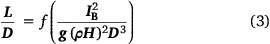
where D is the flame zone depth measured as the short direction of a rectangular flame source or parallel to the fire spread direction, Q′ is the volumetric flow rate of gaseous fuel per unit flame zone width (m³ s⁻¹ m⁻¹), and g (m s⁻²) is gravitational acceleration. Eqn 2 can be written in terms of fireline intensity using Q′=I_B(ρH)⁻¹, in which case:

With further arguments based on entrainment, Thomas showed that if L/D was large, the functional form of Eqn 3 above can be specified as (see section entitled ‘Air Entrainment’ and eqn 11 in Thomas 1963):

where is an empirically determined coefficient into which the constant quantities in Eqn 3 are absorbed. Notice D cancels from Eqn 4, leading to:

which is Thomas’ well known flame length correlation. Thomas (1963) determined the coefficient in Eqn 5 by fitting the equation to experimental flame length data.¹ The absence of D in Eqn 5, along with the goodness-of-fit with experimental data, led Thomas (1963) to reason that effects of D would become negligible when flames were much longer than the flame zone was deep. This conclusion provided theoretical and experimental support for formulating flame length correlations of the form .

Nonetheless, the significant variation among coefficients and exponents among many studies suggests some aspect of the governing physics could be missing. This paper describes an experiment to address this shortcoming by testing the apparent theoretical and experimental support that L is independent of D for a range of fireline intensities and flame zone dimensions. We employed a laboratory sand-burner apparatus that allows precise, independent control of fireline intensity I_B and flame zone depth D from a horizontal fuel source.

This paper reports on experiments conducted on a stationary, propane-fuelled sand burner in an enclosed laboratory. We examine the results in the context of earlier flame length work by Thomas and others and compare with measurements from spreading laboratory fires obtained from prior unrelated studies. The sand burner enabled repeated measurements for an arbitrary length of time, leading to measurement accuracy that would be impossible to achieve on spreading or stationary fires with solid fuels, whether in the laboratory or field. Although the physical processes of solid fuel combustion were absent in a stationary gas burner, the fluid flow, heat transfer processes, and chemical kinetics that lead to observed flame lengths were the same. Propane, along with many other hydrocarbon fuels, burns in non-premixed flaming combustion (diffusion flames) in the same temperature range as gaseous pyrolysates in wildland fires, so it has similar buoyancy. Propane and other hydrocarbon fuel types have different heat contents, stoichiometric air-fuel mixture ratios, and perhaps radiation loss fractions compared with wildland fuels, but compensating effects of each term result in minor variations in flame length compared with the shape, size, and burning rate of the fuel source (Heskestad 1983; Quintiere and Grove 1998).

A propane-fuelled sand burner was constructed at the US Forest Service, Missoula Fire Sciences Laboratory for the purpose of studying flame structure and heat transfer from stationary flame zones (Fig. 1). This sand burner is similar to the one described by Finney et al. (2022) but double the size, having rectangular dimensions of the burner box of 1.22 m × 3.66 m. The sand box was 0.15 m deep with eight perforated tubes running the long axis (3.66 m) along the inside bottom surface under the sand. Sheet metal partitions were sealed with the bottom of the sand box between each burner tube to limit gas diffusion to the 15 cm surrounding each tube. The burner box was mounted on a tilting platform 3.66 × 7.3 m in size, with 4.8 m uphill decking made of flame-resistant Super Fire Temp^®2 board 2.54 cm thick (Johns Manville Corporation, Denver, Colorado, USA, http://jm.com). The downhill decking was 1.2 m (Fig. 1) in length. Each tube was controlled separately for gas flowing from a common manifold so that any combination of tubes could be fired with a controlled flowrate of propane. Gas flow was regulated by an Alicat^® mass flow controller² (Alicat Scientific, Tucson, Arizona, USA, http://alicat.com) capable of flowing up to 1500 standard litres per minute (SLPM) with a stated precision of ±SLPM (meaning 0.42 kW m⁻¹ for our burner). We selected propane flowrates of 300, 600, 900, 1200, and 1500 SLPM for the experiment. Heat release rate (in watts) of the propane flames was determined by multiplying the propane flowrate (in standard litres per minute) by the proportion, 1533 W (SLPM)⁻¹. For example, 600 SLPM propane corresponds to a heat release rate of 600 × 1533 = 919.8 × 10³ W. The conversion factor was calculated by multiplying the density of propane at standard temperature and pressure (1.984 kg m⁻³) and the lower heating value of propane (46.357 × 10⁶ J kg⁻¹), and then dividing by both the number of litres in a cubic meter (1000 L m⁻³) and the number of seconds in a minute (60 s min⁻¹). Thus, (1.984) (46.357 × 10⁶) (1000 × 60)⁻¹ = 1533 W (SLPM)⁻¹.

Fig. 1.  Experimental setup illustrated with (a) picture of propane-fuelled sand burner with gas inlet tubes and short flames, and (b) high speed camera oriented perpendicular to the long-axis of the sand burner and adjusted at height approximately the apparent flame length to minimise parallax. Images by Ian Grob.

These experiments were conducted with the platform oriented horizontally so that length of diffusion flames could be imaged in the pure vertical dimension. Flames from the sand burner were considered buoyancy dominated because the vertical velocity of the propane issuing from the burner surface is very small. To measure flame height, two vertical graduated poles were placed at the foreground edge of the long dimension of the burner in full view of a high-speed camera (Figs 1b, 2). We chose to video the long dimension of the burner because it could more directly incorporate the spatially variable peak and trough structure of line-source flames (Finney et al. 2015), as well as the non-steady and pulsatile dynamics happening at any given location along a linear flame front (Cetegen et al. 1998). The camera was adjusted to the approximate height of the flames at each setting of propane flowrate, with field of view extending the full 3.66 m width of the burner. This ensured that the camera field of view included the expected flame height. The camera captured 10 s of video at 240 frames per second (fps) for each flow rate at each number of open burner tubes (1–8). The camera exposure time was chosen to minimise motion blur from flame movement in each frame.

Fig. 2.  Image processing of flames is illustrated for a 1200 SLPM gas flow rate with 0.3 m flame zone depth D for (a) a single image of flames from video taken at 240 frames per second showing graduated height poles in the foreground, (b) binary image using 90% brightness cutoff for flame presence/absence, (c) contours of flame presence from 10 s of video, and (d) points along the 20% contour corresponding to an average of L = 1.63 m tall (L/D = 5.36). Video stills by Ian Grob.

Measurement of flame dimensions has never been standardised. Studies have relied upon ocular averages or photographic and video methods (discussed by Alexander and Cruz 2012), but all eventually require decisions as to how to delineate luminous flames and for averaging the time and space variation in extent of flames. Absolute comparisons among studies are difficult because of the subjectivity in estimating flame size, the axis of viewing for line fires (long or short dimension, which changes the viewed thickness of the flame profile), and estimates of fireline intensity as discussed in the introduction. In this study, we endeavour to evaluate how a precise and consistent measure of L changes as a function of experimentally controlled flame zone depth. In our case, video was processed to discriminate flaming from non-flaming in each frame using a cut-off pixel brightness value of 90% (Fig. 2b), which filtered much of the illuminated background and foreground objects, including the steel laboratory walls and the decking on the burner apparatus. Individual binary images were then processed to form a flame presence probability field for each fireline intensity–flame depth combination. Contours of flame presence probability were overlayed on a rasterised height gradient matched to the graduations on the reference poles (Fig. 2c). A visual comparison of the video with the probability image suggested that impressions of sustained flame height across the long axis of the burner coincided well with the 20% probability contour. Thus, an estimate of L for a given combination of I_B and D (Fig. 2d) was calculated as the average raster height values from pixels along the 20% contour between the graduated poles to minimise effects on flame length and shape from the lateral edges.

We evaluated the applicability of the flame length–fireline intensity relationship from this gas burner experiment by comparing with data from 100 laboratory fires spreading through laser-cut cardboard fuel beds in wind and on a sloping table (Finney et al. 2013, 2015). The cardboard fuel consists of a ‘comb’ of tines of specified width, separation, and height extending from a common spine normal to the table surface. The spine is embedded in slots in the floor of the burn table, leaving only the tines exposed. The cards can then be installed at any spacing to create exact and repeatable combinations of fuel particle and fuel bed properties (e.g. fuel height, packing ratio, loading).

For these cardboard experiments, fire spread rate was obtained using longitudinal arrays of thermocouples. Flame depth was measured from overhead digital video cameras by counting the rows of cardboard fuel particles burning in the flame zone. These estimates were checked against flame zone depth calculated as the product of measured flame residence time and fire spread rate. Flame length in these studies was estimated ocularly from video cameras and reference height poles or markings on the walls of the wind tunnel. Fireline intensity was calculated from Byram’s equation (I_B = Hm″R) using a heat yield of 13 000 kJ kg⁻¹ for combustion of gaseous pyrolysates (Babrauskas 2006) and 6% fuel moisture content, fuel loading with subtraction of 25% of pre-burn fuel mass for solid residual char and mineral ash (Susott et al. 1975; Di Blasi et al. 2001), and measured spread rate.

The gas burner experiment produced flame length data from a total of 40 combinations of total gas flow rates to the burner (i.e. fireline intensity I_B) and number of burner tubes (i.e. flame zone depth D) (Table 1). Ratios of L/D ranged from 0.14 to 13.6. For any given fireline intensity in Fig. 3a, the flame length decreased with increasing flame zone depth. These relationships were further examined using Eqn 4. However, where Thomas (1963) specified the 1/3 exponent based on theoretical arguments, our analysis allowed for the possibility it could take other values. Nonlinear regression was applied to the experimental gas burner data (Fig. 3b) to obtain the following fit:

which simplifies to illustrate the non-negligible effect of D on L for the burner flames:

and is illustrated in in Fig. 3c. Standard error for the estimated coefficient was 0.001234 and the exponent 0.006852, and all were significant at P < 0.001. The 95% confidence interval for the exponent excluded the 1/3 value reported by Thomas (1963), indicating Eqn 6 is significantly steeper. The narrow confidence bands produced by the strong fit of the regression were nearly indistinguishable from the trend displayed on Fig. 3b; however, the confidence bands for both the fitted model and the model prediction were plotted on the linear axes in Fig. 3c. Five data points shown in open circles in Fig. 3b, c have L/D < 0.52, which Heskestad (1991) established as a criterion for distinguishing single coherent tall fires from ‘mass fires’ composed of multiple short flames, when intensity over the larger fire source is insufficient to form a single flame plume (Thomas 1967; Zukoski et al. 1985). Similar flame structures are evident on the surface of our gas burner with large flame depths, likely explaining why these points show the greatest departure from the regression line. Although not a factor in our experiments, small flames in the laminar range are also unlikely to abide correlations of the taller turbulent flames (Yuan and Cox 1996; Grove and Quintiere 2002).

Table 1.  Table of mean flame length sampled from the video for each combination of fireline intensity and flame zone depth along with standard deviations shown in parentheses.

Fig. 3.  Results of gas burner data (a) for flame length L in relation to fireline intensity I_B compared with correlations by Byram (1959) (Eqn 1) and Thomas (1963) (Eqn 5), (b) the statistical fit of L/D data with the base of Eqn 4 compared with Thomas’ correlation Eqn 4, and (c) L observed vs predicted by Eqn 7, with 95% confidence intervals plotted for the fitted model and the model prediction. Open circles are observations where L/D < 0.52 and flames would likely not form a single plume.

Independent data from spreading laboratory fires (Finney et al. 2013, 2015) showed that when only a function of I_B, L was generally overpredicted by Thomas’ (1963) correlation and underpredicted by Byram’s (1959) at higher intensities (Fig. 4). The data trend was well approximated by the correlation from Eqn 7, where L is a function of both I_B and D. Over much of the data range, predictions from Eqn 7 are significantly different from the correlations of Byram (1959) and Thomas (1963), as indicated by their exclusion from the 95% confidence intervals.

Fig. 4.  Data from 100 laboratory fires spreading with wind or slope show L as a power-function of I_B is generally overpredicted by the relations of Thomas (1963) (RMSE = 0.469) and underpredicted by Byram (1959) at higher intensities (RMSE = 0.349), but well approximated by flame length from Eqn 7 (RMSE = 0.337). Dashed lines show 95% confidence interval of the Eqn 7 model prediction.

The gas burner apparatus allowed precise control over fireline intensity, independent of flame source dimensions, and revealed the important role of D in determining L in these line-source fires. This result contrasts with Thomas’ (1963) data for a similar range (L/D < 7), where the exponent for the fitted correlation in Eqn 4 was found to be 1/3 (Fig. 3b) for L/D > 3 and thus cancelled the influence of D. Steward (1964) also established the theoretical exponent of 1/3 for line fires but experimentally obtained a larger exponent of 0.363 by analysis of a variety of fuel sources for which 2 < L/D < 11. The flame length data assembled by Quintiere and Grove (1998) largely conform to the 1/3 exponent, but only for L/D > 10. Such tall flames with narrow bases are unrealistic for spreading fires in the field and laboratory, suggesting the 1/3 exponent in Eqn 4 is not applicable to flames for which L/D < ~10. Indeed, the following shows that the underlying theory leads one to expect an exponent greater than 1/3 for such fires.

The length of flames is driven by the availability of oxygen for the gas phase chemical reactions of combustion. The familiar yellow–orange flames from wood or hydrocarbon fires are the result of incomplete combustion of the fuel vapour. When insufficient oxygen is present, carbon-rich molecular fuel fragments conglomerate into soot particles, which glow yellow–orange in the intense heat, forming visible flames. When adequate oxygen is available, the fragments are burned to transparent gas. Thus, for a fixed rate of fuel combustion and flame zone size, short flames mean high oxygen availability and long flames mean low oxygen availability.

The process by which oxygen becomes available for combustion in turbulent flames is entrainment. Without wind, ambient air surrounding the flames is drawn into the near field of the buoyant plume. As noted in the Introduction above, Thomas et al. (1961) and Thomas (1963) used an argument pertaining to entrainment to specify the functional form of Eqn 3 as Eqn 4. The argument is briefly summarised here. Dimensional analysis shows non-dimensional flame length for a linear fire source is some function of volumetric fuel flow rate Q′, gravity, and flame zone depth (Thomas 1960; Thomas et al. 1961) as represented by Eqn 2. This can be verified by first noting that the volumetric flow rate of air entrained into flames is the product of the average flow velocity of air entering the vertical flame profile and the surface area of the flame envelope through which entrainment occurs: . Because we are concerned with linear fires, we can reformulate the equation to be on a per-unit-flame-zone-width basis:

Here, A′ is the surface area of the flame envelope per unit W through which entrainment occurs. Fig. 5a–c shows A′ for three idealised flame envelope cross sections for linear fires of the type considered by Thomas et al. (1961) and Thomas (1963). The formulations for A′ appearing below these sub-figures show A′ is proportional to or on the order of D(L/D). We write D(L/D) instead of simply L to more clearly show how Eqn 8 relates to Eqn 2. Therefore, we can write A′ ∝ D(L/D)^p, where p = 1 for the flame geometries in Fig. 5a–c. The exponent p appears here to facilitate the argument following below. Thomas (1963) assumed the total volumetric flow rate of entrainment air into a plume was proportional to the volumetric flow rate of fuel gas leaving the fuel bed (or burner) (i.e. ), and that is proportional to characteristic velocity . Similar entrainment assumptions for the vertical flame profile were made by Steward (1964), Nelson (1980), Grove and Quintiere (2002), and Nelson et al. (2012). Applying these assumptions, Eqn 8 can be rewritten and rearranged to obtain the full functional form of Eqn 2:

When p is set equal to 1, as in Fig. 5a–c, Eqn 9 is readily converted to Eqn 4 by using the fireline intensity substitution used to derive Eqn 3. Because the exponent is 1/3, D cancels from Eqn 4 to obtain:

which is the general form of Thomas’ (1963) flame length correlation (Eqn 5).

Fig. 5.  Cross-sectional profiles of idealised linear flame fronts with equations for A′. Profiles (a–c) are like those considered by Thomas (1963), where A′ ∝ L/D. Natural fires are more similar to profile (d), where A′ is some weaker function of L/D.

Eqn 10 demonstrates that according to the theory presented by Thomas (1963), flame length L is not a function of flame zone depth D when L/D is sufficiently large (thence, p = 1). This being the case, we should expect the flame length data compiled by Quintiere and Grove (1998) to conform to Eqn 5 only when the L/D > ~10, because the flames will exhibit p = 1 geometry. An analogous trend exists for axi-symmetric fires, where L becomes independent of D when L/D > ~3 (Thomas 1963; Heskestad 1983; Zukoski et al. 1985; Grove and Quintiere 2002).

In the absence of wind or slope, line fires with L/D > ~10 have flame profiles that are more acutely pointed and inwardly curved (as in Fig. 5d) due to the horizontal induced flow of entrainment air. Rather than being linearly proportional as before, entrainment area A′ is now some weaker function of L/D. In other words: A′ ∝ D(L/D)^p for 0 < p < 1. Even without the curving profile, Thomas et al. (1961) argued that entrainment for short and wide flames should be proportional to p < 1. Consequently, the exponent of Eqn 9 becomes larger than 1/3 and D no longer cancels out as it did to arrive at Eqn 10. Instead, the equation for flame length is in the form of Eqn 7, meaning that for most spreading natural and laboratory fires, flame length for a given fireline intensity is dependent on D.

The inwardly curved shape of the flame profile in Fig. 5d means that A′ is larger than any of the other profiles for the same flame length, violating the assumption that entrainment and gas combustion occur only along the vertical portion of the flame profile (Steward 1964; Nelson 1980; Grove and Quintiere 2002; Nelson et al. 2012). This means that at least theoretically, there is a larger area over which the plume entrains air and a longer horizontal component of distance that flame gases travel during combustion for a given resulting flame height. The diagrams in Fig. 5 are idealised flame profiles, but real fires with wide bases exhibit curving flame zones in two-dimensional profile and in three-dimensions (Fig. 6). Our analysis was strictly derived from fires without wind or slope but Thomas (1963) reported only minor effects on his correlation for wind-deflected flames. The flame zones of spreading fires, whether in wind or with slope, contain three-dimensional concave flow structures (Fig. 6e–g) created by the downwash of ambient air replacing rising flames and from longitudinal vorticity (Finney et al. 2015; Katurji et al. 2021). These induced circulations increase the exposure of flame gases to ambient air within deeper flame zones.

Fig. 6.  Images of flame profiles from gas burner flames with I_B = 246 kW m⁻¹. (a) D = 0.15 m, (b) D = 0.46 m, (c) D = 0.76 m, (d) D = 1.07 m showing smaller flames and increased curvature with wider flame base and reduced L/D. Oblique overhead images of heading fires showing concave flame circulations within flame zones of (e) a laboratory fire in laser-cut cardboard (L = 0.4 m; D = 0.4 m; L/D ≅ 1; Finney et al. 2015), (f) crop stubble fire (L ~ 5 m; D ~ 10 m; L/D ≅ 0.5), and (g) gorse brush fire in New Zealand (L ~ 15 m; D ~ 30 m; L/D ≅ 0.5).

Comparisons of the gas burner model (Eqn 7) with laboratory data from wind and slope-driven fires over a similar range of I_B, L and D (Finney et al. 2013, 2015) show that the model was applicable to spreading fires (Fig. 4). We do not have independent confirmation of scaling beyond this range of flame lengths or intensities, but for spreading fires, Eqn 7 will generally produce lower estimates of L than Thomas’ (1963) correlation because of the significant influence of D. The deeper flame zones of surface fires may offer some explanation for preferred applicability of Byram’s correlation for heading fires (Albini 1976). Indeed, Thomas (1971) reported that his laboratory-based correlation (Eqn 5) overpredicted flame lengths observed from a variety of burns in grass, gorse, and heather, although he dismissed the influence of D on those discrepancies. Nevertheless, Eqn 5 was adopted for use in crown fires (Rothermel 1991) because Eqn 1 underpredicts tall flames (Byram 1959). Further analysis and data will be required to determine if Eqn 7 from this study applies to both surface and crown fires.

Histograms of L/D ratios from six data sets representing spreading fires in laboratory and field conditions show values of L/D < 2 for a variety of fuel and fire types (Fig. 7). In spreading fires, flame zone depth varies within the same fuel type because the flame zone geometry cannot be controlled independently from spread rate and frontal intensity. The exception occurs for fires backing into the wind (and those without wind on flat ground) that have much narrower D than fires heading with the wind (Beaufait 1965). Data from Catchpole et al. (1998a) show median L/D ratios for laboratory no-wind fires were 1.8 compared with 0.55 for heading fires (Fig. 7c). The no-wind fires of Wilson (1990) show the highest median values (2.478) among all data sets examined (Fig. 7e).

Fig. 7.  Histograms of L/D ratios for various data sets from spreading fires show generally higher values for fires with no wind compared with heading fires (* indicates significantly different median values based on the Kruskal–Wallis test for data from Catchpole et al. (1998a)). Fire behavior data from burns in (a) cardboard fuel arrays under laboratory wind and slope conditions (Finney et al. 2013, 2015), (b) pine needles under field conditions (Nelson and Adkins 1986, 1988), (c) excelsior, pine needles and pine sticks under laboratory conditions (Catchpole et al. 1998a), (d) grass under field conditions (Sneeuwjagt and Frandsen 1977), (e) excelsior and pine sticks under laboratory conditions (Wilson 1990), and (f) southern rough and needle fuel complexes under laboratory and field conditions (Nelson et al. 2012).

Among 28 published L–I_B correlations (Table 2), those for backing and no-wind fires yielded higher flame length for a given intensity than heading fires (Fig. 8a). Three studies reported L–I_B relations for backing fires with higher exponents than heading fires (2/3 vs 1/2, Nelson (1980); 0.724 vs 0.543, Fernandes et al. (2009); and 1.75 vs 0.99, Clark (1983)). However, flame length for a given intensity is a non-unique combination of the exponent and coefficient that is illustrated by a plot of these terms for all studies in Table 2 (Fig. 8b). Backing and no-wind fires have a higher exponent for a given coefficient, and a higher coefficient for a given exponent, than heading fires, and in combination lead to higher flame lengths for a given intensity. This illustrates that some variation among correlations can originate from the statistical ambiguity of curve fitting by linear or nonlinear regression, which can yield various combinations of coefficients and exponents with reasonable goodness-of-fit to experimental data. For example, instead of fitting both terms, Nelson et al. (2012) relied on the analytically derived 2/3 exponent from Thomas (1963) and only fit the coefficient.

Table 2.  Published correlations of flame length with fireline intensity.

Fig. 8.  Graphs of L–I_B correlations in Table 2 for backing and no-wind fires (red) grouped separately from heading fires (black) (a) compared with hypothetical L/D ratios from Eqn 7 in open squares, and (b) showing that backing and no-wind fires have higher exponents for given coefficient and higher coefficient for a given exponent than heading fires (note that correlations from Clark (1982) are not plotted). Data from Vega et al. (1998) for mixed heading, backing, and flanking fires are represented by the dashed line in (a) and open circle in (b).

The variability among published L–I_B relations (Table 2, Fig. 8a) has invited numerous interpretations. Comparisons among studies are made difficult by the non-steadiness of flames and absence of standardised methodology for measuring flame length (Zukoski et al. 1985; Newman and Wieczorek 2004; Alexander and Cruz 2012). Biases can also arise in the fireline intensity estimates from Byram’s (1959) equation (I_B = Hm″R). The spread rate R (m s⁻¹) may not be constant (Santoni et al. 2010) and the heat yield H (kJ kg⁻¹) may be overestimated if heat losses for radiation, moisture evaporation, and incomplete combustion are improperly accounted for (Byram 1959; Nelson and Adkins 1986) or if values of H are averaged for the gas phase and solid phase combustion (Susott et al. 1975; Babrauskas 2006). A well-known problem in wildland fire research is overestimating the fuel mass per unit area consumed in flaming m″ (kg m⁻²). This occurs when the measured fuel mass consumed in an experiment is attributed solely to flaming combustion, whereas in reality, both flaming combustion and solid phase combustion were responsible. The result of such an assumption is I_B is calculated to be too high for observed L. To avoid this, Santoni et al. (2011) used O₂ calorimetry in a spreading laboratory fire to estimate I_B and the technique was subsequently employed by Barboni et al. (2012) as well. However, it is possible that residual combustion behind the spreading front may still affect measurement of heat release and lead to an exaggerated I_B.

To examine the possible role of D as a source of the variability in L–I_B correlations, we assumed from the congruence of burner data with Thomas’ (1963) correlation (Fig. 3a) that Eqn 5 was correct in the limit of large L/D. Hypothetical estimates of D could then be derived as a constant ratio of calculated L, and when used in Eqn 7, enabled comparison with published correlations (Fig. 8a). Although the L/D ratio is actually not constant for any given fuel type or range of intensity (Fig. 7), this exercise suggested that a substantial portion of variability among L–I_B correlations was covered by the range of hypothetical L/D ratios: from 0.5 to 50 (Fig. 8a). Low L/D ratios of 0.5 and 1.0 (see examples in Fig. 6) approximated many heading fire equations, including Nelson and Adkins (1986) and Byram (1959). The middle range of L/D from 4 to 10 are similar to the no-wind fires by Thomas (1963), Fons et al. (1963), and Barboni et al. (2012). The highest L/D ratio of 50 was in the range of burner data presented by Yuan and Cox (1996), where L was 30–100 times the 0.015 m burner D. Not all of the variability among L–I_B relations was within the hypothetical L/D limits, however, and the correlations showing low flame lengths for a given intensity suggest a contribution of other factors in determining L and I_B as discussed above, particularly those that would inflate the value of I_B.

A significant effect of D on L also leads to a previously unreported negative feedback mechanism that limits the spread rate of wildfires. Negative feedbacks are clearly implicated in limiting fire spread rate because the magnitude of spread rate and intensity reach a steady state after increasing rapidly immediately following ignition (McAlpine and Wakimoto 1991; Cheney and Gould 1997). We had earlier reported on the role of D in reducing convective heating by diminishing the gas temperature profile adjacent to the flaming edge (Finney et al. 2021, 2022). A similar effect of D on L shown here would decrease radiation view factor and reduce scaling of processes dependent upon flame length, including flame velocity. Both effects of D would work together to dynamically limit fire spread rate as the flame zone depth extends further behind the edge of an accelerating fire.

Experimental data from a propane sand burner demonstrated that flame zone depth D significantly reduces flame length in relation to fireline intensity in the range of 0.14 ≤ L/D ≤ 13.6. The data were analysed in context of Thomas’ (1963) dimensionless flame length formulation to obtain a new correlation that included D, which was then found to improve the fit to a data set from spreading fires. The general implications of these findings were examined using 28 published correlations and their experimental characteristics, confirming reports that backing fires (and those with no wind) had higher predicted flame length than heading fires for a given intensity. This is consistent with the effect of narrower flame zone depth D of backing and no-wind fires made apparent by the new flame length correlation. Other sources of variation likely include the well-known uncertainties involving measurement of flame length, spread rate, or fireline intensity. The low L/D ratios found in wildland fires compared with those idealised for line fires by theory of entrainment and gas combustion mean that a substantial proportion of the variability in reported flame length correlations would be reduced if flame depth was accounted for.

Data are available upon request from the authors.

The authors have no conflicts of interest.

The study was funding by the US Forest Service, National Fire Decision Support Center.

References

Albini FA (1976) Estimating wildfire behavior and effects. General Technical Report INT-GTR-30. (USDA Forest Service, Intermountain Research Station: Ogden, UT)Alexander ME (1982) Calculating and interpreting forest fire intensities. Canadian Journal of Botany 60, 349–357.