

Environmental conditions on the Pacific halibut fishing grounds obtained from a decade of coastwide oceanographic monitoring, and the potential application of these data in stock analyses
Lauri L. Sadorus A , Raymond A. Webster A * and Margaret Sullivan B
A
B
Abstract
Establishing baseline environmental characteristics of demersal fish habitat is essential to understanding future distribution changes and to identifying shorter-term anomalies that may affect fish density during monitoring efforts.
Our aim was to synthesise environmental data to provide near-bottom oceanographic baseline information on the Pacific halibut fishing grounds, to establish geographic groupings that may be used as co-variates in fish-density modelling and to identify temporal trends in the data.
Water-column profiler data were collected from 2009 to 2018 along the North American continental shelf, during summer fishery surveys focused on Pacific halibut.
In addition to establishing baseline information on the fishing grounds, this analysis illustrated that environmental variables can be grouped geographically into four regions that correspond to the four biological regions established by the International Pacific Halibut Commission. A spatio-temporal modelling approach is presented as an example of how to describe the relationship between environmental data and Pacific halibut distribution.
This study has highlighted the efficacy of environmental data in analysing fish distribution and density changes.
Oceanographic monitoring provides the ability to detect annual anomalies such as seasonal hypoxic zones that may affect fish density and to establish baseline information for future research.
Keywords: chlorophyll-a, dissolved oxygen, environment, geostatistical model, monitoring, North Pacific Ocean, Pacific halibut, salinity, temperature.
Introduction
Oceanographic data are collected on various scales and by a variety of means throughout the North Pacific Ocean. This has led to the creation of long-term datasets, such as the Line P transect in British Columbia waters where oceanographic data have been collected since 1956 (Tabata and Weichselbaumer 1992), National Oceanic and Atmospheric Administration (NOAA)-facilitated moorings in the Gulf of Alaska, Bering Sea and Aleutian Islands with some in operation since the early 1990s (National Oceanic and Atmospheric Administration, Pacific Marine Environmental Laboratory 2022), and gliders deployed throughout the world’s oceans that collect water-column profiles as they also move horizontally through the water (Dunbabin and Marques 2012). Additionally, some studies have considered oceanographic variables alongside species catch and distribution (e.g. Keller et al. 2017), or species distributions in relation to climatic conditions (Stevenson and Lauth 2019). The first 10 years of coast-wide oceanographic data collection by the International Pacific Halibut Commission (IPHC) provides a solid foundation for describing environmental conditions experienced by older juvenile and adult Pacific halibut in the early part of the 21st century. The IPHC coincident dataset is unique in that it provides a surface to near-bottom water-column profile of five key oceanographic variables at each fishing station annually, beginning in 2009. Not only can this provide information to support studies of large-scale environmentally driven organism distribution shifts over time, but also informs the study of small-scale, regional responses of Pacific halibut to various oceanographic changes. In addition to being uniquely coincident with Pacific halibut catch data, the IPHC oceanographic dataset contributes to the larger picture of documenting oceanographic characteristics in the North Pacific Ocean and Bering Sea when used alongside other scientifically collected oceanographic data. Many other fishery surveys conducted in the North Pacific Ocean collect elements of oceanographic data, most often temperature. For example, the NOAA groundfish bottom-trawl surveys in the northern Pacific and Bering Sea routinely collect surface and bottom temperature while fishing (National Oceanic and Atmospheric Administration 2022), providing a coincident data set that can be used in climatological studies and stock assessments.
Beginning in 2009, the IPHC annually profiled the continental shelf water column in summer, collecting surface to near-bottom pressure, conductivity (salinity), temperature, dissolved oxygen (DO) concentration, pH and fluorescence measurements. The profiling instruments (Seabird Scientific Model SBE19plus) were deployed from the Fishery Independent Setline Survey (FISS) platform (Ualesi et al. 2021), which is a longline survey that annually fishes stations throughout the IPHC Convention Area (Fig. 1). The FISS primary target, Pacific halibut (Hippoglossus stenolepis), is a demersal flatfish, so the bottom-most measurements from the profilers are presumed to be indicative of the conditions experienced by the fish caught on the FISS gear at that location. Extensive environmental monitoring during the FISS allows for the possibility of using environmental covariates as inputs to the Pacific halibut stock-assessment process and examination of fish distribution during historically average conditions as well as during conditions outside the historic ranges. Understanding the baseline environmental habitat and associated variability is essential to future analyses.
IPHC Regulatory Areas used for management are shown in grey and Biological Regions used to study Pacific halibut stock components are indicated in blue for the North Pacific Ocean and Bering Sea.
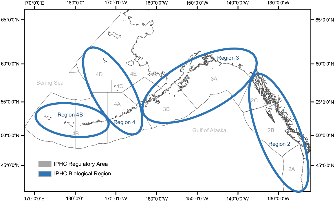
Currently, the North American Pacific halibut fishery is managed by a set of Regulatory Areas (Fig. 1) where boundaries are based on political and management requirements, but do not necessarily correspond to natural biological groupings within the stock (Hicks and Stewart 2018). Hicks and Stewart (2018) found that grouping the Regulatory Areas into four Biological Regions, as outlined in Fig. 1, helps explain the subpopulation structure within the larger stock during analyses. These regions are similar to marine regions identified in Link and Marshak (2019) for the exclusive economic zone of the USA in the North Pacific Ocean. Within regions, Pacific halibut has similar biological and population processes such as migration patterns, sex ratios, age compositions, size at age and historical trends that, when grouped together, make up the factors governing bio-complexity. Preserving bio-complexity of a stock may buffer against population declines in a variable or changing environment (Hilborn et al. 2003). The IPHC environmental data-collection program provides an opportunity to examine whether these Biological Region designations also encompass similar groupings of distinct oceanographic conditions experienced by Pacific halibut on the fishing grounds, such that environmental co-variates may be used in analyses focusing on the preservation of stock bio-complexity.
Recent climate-related environmental changes, particularly in temperature, have been correlated with marine species movement outside normal ranges of distribution, and model projections under various climate-change scenarios adopted by the Intergovernmental Panel on Climate Change (2014) have shown that species response to increasing temperatures will generally be poleward as the oceans warm (Morley et al. 2018). Examples of these movements are numerous. Selden and Pinsky (2019) found that many marine species around the globe can adapt quickly to changing ocean conditions such as temperature, and this adaptation in recent years has resulted in northward relocation for some species as waters warm. In the Bering Sea, Stevenson and Lauth (2019) found that certain species shifted further north in warm stanza years, compared with cold stanza years (Sigler et al. 2016), on the basis of results from the NOAA Alaska Fisheries Science Center (AFSC) summer bottom-trawl survey. Off the coast of Australia, Smith et al. (2019) documented a poleward shift of a whiting species (Sillago schomburgkii) beginning in 1950, which corresponded temporally to increasing ocean temperatures in the region. In that study, an intensification of temperature during a marine heat wave in 2010–2011 led researchers to conclude that geographically driven spawning successes and failures were causing the redistribution, as opposed to the movement of adults to more hospitable habitat. Oxygen deficits have also been shown to initiate species distribution shifts when DO concentrations drop below the minimum tolerance for an animal and if that organism possesses the ability to respond appropriately, including relocation to more oxygenated waters just outside the hypoxic zone or migration out of the area altogether (e.g. Diaz 2002; Chan et al. 2008). Monitoring responses to environmental factors may be relevant to local ecosystem dynamics and to properly interpreting spatial and temporal-based distribution differences seen in the related fisheries and scientific surveys.
The IPHC uses the output of spatio-temporal modelling of Pacific halibut survey data to estimate time series of Pacific halibut density indices, which are then used as an input to the annual Pacific halibut stock assessment (Stewart et al. 2019), and to estimate the distribution of the stock among IPHC Regulatory Areas and Biological Regions (Hicks and Stewart 2018). This modelling approach is useful for interpreting survey results for Pacific halibut, because it attempts to estimate the underlying density process, smoothing the data in time and space by accounting for temporal and spatial correlation. It also permits prediction into locations not covered by the survey stations in a given year. Although the IPHC does not currently use environmental covariates as a direct input to the stock assessment, integrating such information into the spatial–temporal models of density indices is more straightforward (e.g. Boudreau et al. 2017; Essington et al. 2022). Including environmental covariate data as model inputs has the potential to increase the understanding of ecological processes and interactions (Koenigstein et al. 2016), and improve the general understanding of the drivers of shifting fishery distribution that are important to managing the resource (Selden and Pinsky 2019). Environmental covariate data have been used successfully in recent studies of fish distribution (e.g. Ibaibarriaga et al. 2013; Bitetto et al. 2019; Essington et al. 2022). In the current work, we have examined the efficacy of using environmental variables as covariates in the spatio-temporal modelling of Pacific halibut survey data by the IPHC. We anticipate that using environmental data in this way will help identify the environmental causes for unexpected distributional changes that otherwise may be difficult to interpret or are potentially mis-attributed to other factors (e.g. random variation, fishing vessel differences).
The results of this work will fulfill the following objectives: (1) establish baseline environmental data for North American Pacific halibut habitat for older juvenile and adult animals, (2) evaluate oceanographic-variable characteristics in relation to IPHC Biological Regions, (3) understand recent oceanographic changes on the Pacific halibut grounds, (4) through an example, evaluate the possible application of profiler data in spatio-temporal modelling that is used in the Pacific halibut stock assessment.
Materials and methods
Oceanographic instrument deployment
Seabird SBE19plus profiling units were deployed just prior to hauling the longline fishing gear at each FISS station from 2009 to 2018. The FISS was conducted using chartered longline fishing vessels that deployed standardised longline gear and bait during the summer months (primarily June, July and August) along a grid of fishing stations located on the continental shelf. Profiles were collected during periodic range expansions into areas and depths not ordinarily sampled, but only data from those stations scheduled to be profiled in all years (i.e. core stations) were retained for this analysis. The profiling instruments were equipped with sensors that collected measurements of pressure (decibars were used as a shallow-water proxy for depth in metres), conductivity (from which salinity in practical salinity units, PSU, were calculated), temperature (°C), dissolved oxygen (DO, mL L−1), pH and fluorescence (mg m−3; indicating chlorophyll-a concentration). A pump ensured consistent sampling throughout the profile. An anchor weight was attached by 15 m of the fishing vessel’s buoy line to the bottom of the stainless-steel cage that surrounded the instruments. Attached to the top of the cage was a float assembly and buoy line that remained secured to the fishing vessel throughout deployment (Fig. 2).
Schematic of the water-column profiler set-up used for oceanographic sampling during the IPHC fishery-independent setline survey. The unit is equipped with floats attached to the top of a protective frame and a weight attached by buoy line to the bottom of the frame to ensure a vertical descent and to minimise the risk that it will affect the bottom.
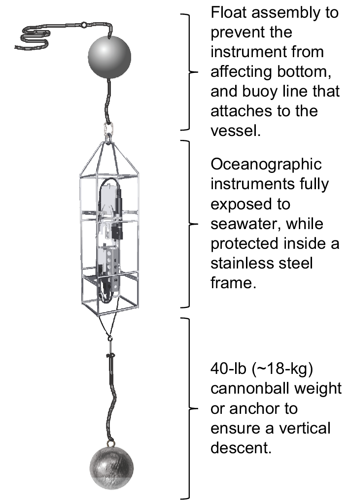
Once on station and prior to hauling the longline gear, the profiler assembly was deployed. The float and weight rigging was designed to accomplish a vertical descent of 1–2 m s−1. Data were recorded at a rate of four readings per second, and were uploaded periodically to onboard computers. Both in-season and annual maintenance was performed on the instruments as recommended by the manufacturer. In 2012, the anchors of the profiling units were equipped with an additional depth sensor (Star-Oddi DST logic model) and analysed in conjunction with the profiler-depth and vessel-depth sounder instruments to estimate proximity of the profiler to the sea floor at its deepest reading. The analysis produced an estimate that the instruments came within 5–15 m from the bottom, on average, depending on total depth of the station and likely other factors such as horizontal-current strength (Sadorus et al. 2016).
Data conversion and preliminary data-quality assessment and control (QC) of the profile data were accomplished using Seabird Scientific’s software SBE Data Processing (ver. 7.26.7, see https://software.seabird.com/). Profiles were averaged to 1-m bins. No calibration water samples were collected because of FISS limitations, and variables were not laboratory calibrated. Data were visually inspected and QC-edited as needed post-season. Initial accuracy for the instruments used was as follows: pressure (+0.1% of full-scale range), temperature (+0.005°C), conductivity (+0.0005 S m−1), dissolved oxygen (+2% of saturation) and chlorophyll-a (sensitivity of 0.02 μg L−1). Temperature data rarely fell outside set parameters and the sensors proved stable. Most problems with salinity data occurred in the upper water column, and values were stable in the deeper water layer where the majority of Pacific halibut habitat occurs. Oxygen and chlorophyll-a values would likely have been improved with in-season calibration, but were stable overall, i.e. the sensitivity of the instruments did not appear to drift considerably between annual calibrations. The pH data are useful as a general indicator, but are the least reliable of these data and were not included in this analysis, because the pH sensors were known to have drift problems. Full profiler datasets for each year are available for download from the IPHC website (see https://www.iphc.int/datatest/data/water-column-profiler-data), and near-bottom measurements for temperature and DO are also available on the website using the FISS data-visualisation tool (see https://www.iphc.int/data/FISS-catch-per-unit-effort).
Oceanographic and catch data
Because Pacific halibut is demersal, the deepest readings at each station were the most indicative of conditions that the animals in that area were experiencing. Profiles were excluded from this analysis if it was suspected that the instrument failed to reach the bottom. The profiler data for pressure, temperature, DO and salinity were averaged and binned into 1-m depth increments, checked for accuracy, and the deepest binned values for each profiler cast were used in this analysis. Averaging of near-bottom data included only those stations that had been profiled successfully five or more times during the 10-year period. Profiler data from 2009 to 2014 were pre-processed by IPHC and, subsequently, underwent rigorous quality control (QC) processes by the NOAA Pacific Marine Environmental Laboratory (PMEL) in collaboration with the University of Washington Joint institute for the Study of the Atmosphere and Ocean (UW, JISAO) (Sadorus et al. 2016). More rigorous QC included the use of various tools to account for pressure reversals owing to weather and sea conditions, to align data relative to pressure, and to derive variables (salinity, density, σt, oxygen saturation). Data from 2016 to 2018 were processed at the IPHC only.
Chlorophyll-a measurements were averaged within each 1-m depth bin (there were typically 3–5 measurements per bin), so as to smooth any anomalous readings that may have been due to movement of the profiler in the current. Depth-integrated chlorophyll-a density at each station was estimated by using numerical integration with the trapezoidal rule over the station depth range, by using the 1-m averages as input data. Thus,
where xi, i = 0, …, n, is the ith depth with mean chlorophyll-a value of f(xi). In our case, , since n, the number of depth bins, is equal to the depth (m), which equals b1 – b0, the difference between the greatest and smallest (b0 = 0) depth at a station. This calculation yielded chlorophyll (mg m−2) throughout the area. Station outliers were examined by inspecting the chlorophyll-a pattern across all depths for that station for reasonable values and by comparing to nearby stations. Data that did not fit into the pattern examined were removed. Prior to the calculation, slightly negative readings within the casts resulting from calibration differences of the sensor were changed to zero. Only those stations that had been fished five or more times during the 10-year period were included.
The spatio-temporal modelling included near-bottom temperature and DO data collected by the profilers and Pacific halibut catch data, which were recorded during the FISS and uploaded to the IPHC relational database post-season (catch data available at https://www.iphc.int/data/FISS-catch-per-unit-effort). Catch data were standardised to weight-per-unit-effort (WPUE) of Pacific halibut with fork length at least 81.3 cm (~32″, the commercial fishery size limit), i.e. pounds caught per 1800-foot (~1645-m) skate of fishing gear (International Pacific Halibut Commission 2020).
In total, 10,573 surface-to-bottom useable-quality profiles were collected for this analysis over the 10-year period from 2009 to 2018. In any given year, a small number of profiler deployments were missed because of poor weather or data were discarded post-season because of sensor malfunction. Following the editing process, 1268 unique stations remained for use in the analysis, each station having had five or more useable profiles over the study period. For the spatial-modelling example of hypoxia (defined here as DO < 1.4 mL L−1) off the western coast of USA, all viable stations were included regardless of the number of times they were sampled over the 10-year period, such that all useable data available for 2017 and 2018 (years when additional stations were fished in IPHC Regulatory Area 2A) were utilised.
Statistical analysis
The oceanographic variables of temperature, salinity, DO and depth-integrated chlorophyll-a were compared across regions and over the 10-year time period by fitting linear models (function lm in the ‘stats’ package in R, ver. 3.6.1; see https://stat.ethz.ch/R-manual/R-devel/library/stats/html/00Index.html). Residual plots showed that the underlying model assumptions were met for the temperature and DO data and no prior data transformation was required. Chlorophyll-a data were highly skewed and normality and variance stability (homoscedasticity) were improved with a fourth-root transformation; although these transformations may lack a biological motivation, they were necessary for insuring the validity of the statistical inference. Model assumptions were violated for salinity data regardless of any transformation. Therefore, the untransformed-data curves were determined to provide the most useful description of the time-series. Of those variables examined, overall time trends and comparisons among biological regions were estimated by fitting a sequence of increasing complex linear models (Kunter et al. 2004), with F-tests and Akaike’s information criterion (AIC, Akaike 1973) used to select the best-fitting model. Analyses were performed in R (ver. 3.6.1, R Foundation for Statistical Computing, Vienna, Austria, see https://www.r-project.org/). We fitted models that assumed a simple linear relationship with time within each biological region over the 10-year data period, because our goal was to understand overall temporal trends (i.e. determining whether the means of these variables were increasing or decreasing, on average, over time), while recognising that variation over time is more complex than a simple linear process (see Supplementary Fig. S1–S4 for raw data plots).
Spatio-temporal modelling
Spatio-temporal modelling allows for the integration of environmental information as covariates within models for catch rate, while accounting for spatial and temporal correlation among the observations. Specifically, we used a delta-type model (Shelton et al. 2014) in which the probability of catching zero fish and the distribution of non-zero catches are modelled as connected spatio-temporal processes for recent data from IPHC Regulatory area 2A. This area was chosen to illustrate the potential usefulness of including environmental covariates in such models for Pacific halibut for the following two main reasons: its small size means we can fit spatio-temporal models quickly relative to other management areas, and notable recent hypoxic events mean we have a least one covariate that spans a range of values likely to have a clear effect on Pacific halibut density.
The dependent variable in our models is weight-per-unit-effort (WPUE), the catch weight of Pacific halibut with fork length 81.3 cm and over (the commercial size limit) divided by the number of 100-hook skates set. Whereas we recognise that WPUE is a function of both density and catchability, for the purpose of this analysis, we are assuming that WPUE provides an index of Pacific halibut density (see Discussion). Let w(s,t) be the IPHC FISS WPUE value at location s (a vector of coordinates) in year t, where s represents the spatial locations of the fished survey stations, taking values s1, …, sn (vectors of coordinates) and t = t1, …, tT. In our model, each si ε S2, the set of points on the surface of a sphere. Data from the FISS contain observations of zero WPUE, owing to stations in low-density areas catching no Pacific halibut. Two new variables are defined, x(s,t) for presence or absence of Pacific halibut in the catch and y(s,t) for the WPUE value when Pacific halibut is present, as follows:
The NA indicates that y(s,t) is a random variable that can take only non-zero values, and is therefore undefined when w(s,t) = 0. The variable x(s,t) has a Bernoulli distribution, x(s,t) ~ Bern(p(s,t)), whereas a gamma distribution is used for the y(s,t), y(s,t) ~ gamma(a(s,t), b(s,t)), which has mean μ(s,t) = a(s,t) ÷ b(s,t). The gamma is parameterised in terms of the mean and variance, with only the former allowed to vary; the variance ( = a(s,t) ÷ b2(s,t)) is assumed constant over space and time.
Next, let the ε(s,t) be a Gaussian field (GF) that is shared by both component random variables in the following way:
The parameter βε is a scaling parameter on the shared random effect. Environmental covariates are introduced into each model component through fx() and fy(), functions of a spatially and temporally indexed covariate data matrix (z) and covariate vectors βx and βy.
Temporal dependence is introduced through a simple autoregressive model of order 1 (AR(1)), as described in Cameletti et al. (2013), as follows,
where ρ denotes the temporal correlation parameter and |ρ| < 1. For a given year, t, the spatial random field, η(s,t), is assumed to be a Gaussian field with a mean zero and covariance matrix Σ. We assume a stationary Matérn model (Cressie 1993) for the spatial covariance model, which specifies how the dependence between observations at two locations decreases with an increasing distance.
Two covariates that appear linked to Pacific halibut density were included in the models for data from IPHC Regulatory area 2A, namely, bottom temperature and DO. Models were fitted with either linear or quadratic relationships for temperature, because data exploration throughout the species’ range indicated that Pacific halibut density can be negatively affected by both extremely low and very high temperatures. Thus, for temperature, the most complex model considered included as part of fx() in Eqn 1 and as part of fy() in Eqn 2, where T = T(s,t), the bottom temperature measurement at location s and year t. We also considered linear and quadratic models for the relationships with DO; even though we do not have much data for either the very lowest or highest values of DO, a linear function did not appear to adequately describe the relationship. Thus, βx3DO + βx4DO2 were added as part of fx() and βy3DO + βy4DO2 as part of fy(). Finally, we also fitted a model with a different intercept term for DO with values less than 0.9 mL L−1, which past and current data imply is a cut-off level in DO below which Pacific halibut catches are almost always zero (Sadorus et al. 2014). This meant adding the term βx5I(DO < 0.9) to fx() and βy5I(DO < 0.9) to fy(), where I() is the indicator function taking value one when its argument is true and the value zero otherwise. A similar ‘breakpoint’ model was fitted by Essington et al. (2022) to sablefish (Anoplopoma fimbriadata) data off the western coast of USA, although they estimated the cut-off level within the model.
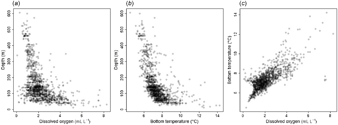
Models were fitted in a sequence (Table 1), starting with a ‘base’ model that included depth, a binary variable for latitude (1 if <40°N, 0 otherwise), and a temporal-trend effect; this is the model the IPHC fits annually for the purposes of producing a density index for use in the stock assessment. We model both the depth relationship and the trend in a flexible manner by a random-walk process as described in Webster et al. (2020). We note that depth, temperature and DO are correlated (Fig. 3), potentially making it more difficult to interpret the results of the modelling; both higher bottom temperatures and higher DO concentrations are found in shallower waters, although the lowest DO values also most commonly occur in depths from 0 to 200 m. This was managed through the sequential model fitting and selection process, which allowed us to compare the fit of models with and without each covariate. The latitude covariate is to account for extremely low-density habitat at the southern limits of the species’ range that was surveyed only once in 2017; its inclusion means that the low WPUE predictions south of 40°N persist throughout the time series, whereas predictions in this region would otherwise drift towards the long-term mean.
| Model | Bottom temperature | DO | |
|---|---|---|---|
| A – base model | – | – | |
| B | Linear | – | |
| C | Quadratic | – | |
| D | Quadratic | Linear | |
| E | Quadratic | Quadratic | |
| F | – | Quadratic | |
| G | – | Quadratic; intercept differs for DO < 0.9 mL L−1 |
Plots of (a) depth against dissolved oxygen, (b) depth against bottom temperature and (c) bottom temperature against dissolved oxygen, as recorded by IPHC water-column profilers in the IPHC Regulatory Area 2A FISS from 2009 to 2018.
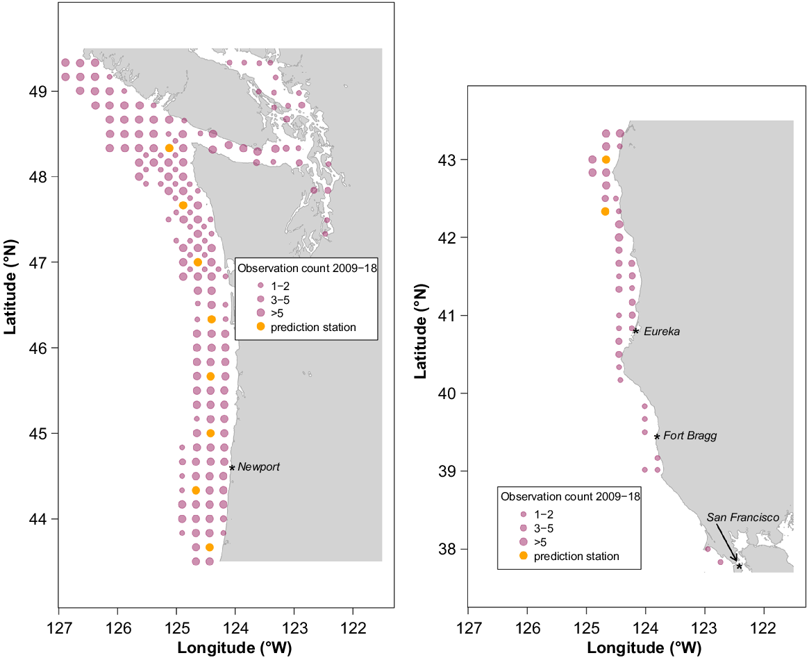
Some station data from the southern end of adjacent IPHC Regulatory Area 2B were included in the space–time models because spatial dependence extends beyond the regulatory-area boundaries and, therefore, such data provide additional information for IPHC Regulatory Area 2A models. In total, 1265 observations from 2009 to 2018 were used in the space–time modelling. Fig. 4 shows station locations, with circle size indicating the sampling frequency over the 10-year period.
Maps showing location of stations, with data used in the space–time modelling that were collected during the IPHC FISS. Circle size indicates the number of times each station was both successfully fished and produced valid water-column profiler data. Stations selected for model prediction are shown in orange.
Models were fitted in R using the R-INLA package (ver. 22.12.16, see https://www.r-inla.org/; Lindgren and Rue 2015), which uses a computationally efficient Bayesian approach to fitting spatial and spatio-temporal models. Further details are available in Webster et al. (2020), which includes a description of the process we used for creating a non-convex triangulated mesh for the habitat region of interest used by the INLA approximation in the models. Independent, non-informative prior distributions were used for the model parameters, including Gaussian priors for fixed effects and log-gamma priors for variance parameters.
The fits of the models were compared using the deviance information criterion (DIC, Spiegelhalter et al. 2002) and a k-fold cross-validation. For the latter, the data were divided into k = 5 subsets of equal size. The models were then refitted with one subset omitted, and the refitted model was used to obtain predictions of WPUE (posterior means) for each omitted observation. This process was repeated for each of the five subsets, providing a prediction for each observation in the original data set. An overall measure of model fit was then computed as the mean square error, as follows:
where and are the ith observed and predicted values of WPUE and N is the total number of observations used in the modelling.
To help compare the observed data with modelled covariate relationships, we selected 10 prediction stations spanning the latitude range of the core of the IPHC Regulatory Area 2A stock north of 42°N (shown as orange circles in Fig. 4). Means of posterior predictions for these stations for 2013 (chosen as it was an ‘average’ year for mean WPUE over the 2009–2018 period) over a range of covariate values were calculated and plotted for the best-fitting models.
Results
Measured environmental variables
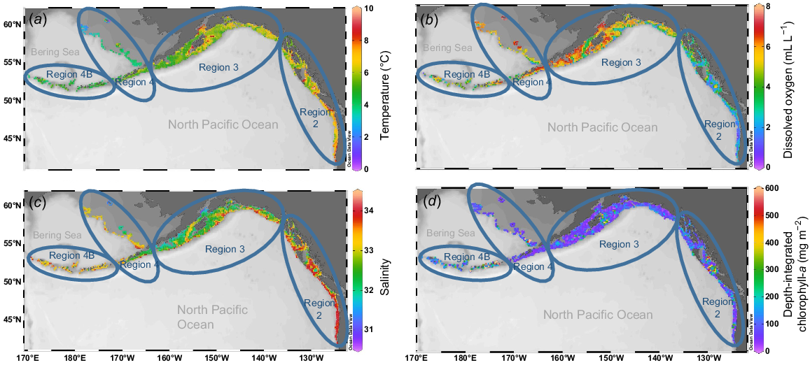
Mean station bottom temperatures over the study period (2009–2018) ranged from 0.4 to 10.1°C, with the highest temperatures consistently occurring off the western coast of USA, and off Vancouver Island, British Columbia, Canada in Biological Region 2, and around Kodiak Island, Alaska, USA, in Biological Region 3 (Fig. 5a). Coldest mean near-bottom temperatures by station were found in the Bering Sea, particularly at stations surrounding St Matthew Island and along the northern Bering Sea continental shelf edge in Biological Region 4. The highest regional mean temperature overall was in Biological Region 2 and the lowest in Region 4 (Fig. 5a; Tables 2 and 3). Region 4 displayed the greatest variability among biological region station means, and Region 4B displayed the smallest range of variability (Fig. S1). Mean temperatures over the study decade varied, but there was strong evidence that the overall trends varied among regions (Table 4a), with a greater average increase in Biological Region 4 than other regions (Fig. 6a). A recent study (Amaya et al. 2023) examining bottom temperatures in the Gulf of Alaska and Bering Sea supports the finding that the Bering Sea experienced higher average intensities of marine heatwave temperatures than in the Gulf of Alaska.
Maps showing mean oceanographic conditions for each station profiled for the Years 2009–2018 during the IPHC FISS: (a) near-bottom temperature (°C); (b) near-bottom dissolved oxygen (mL L−1); (c) near-bottom salinity (PSU); (d) depth-integrated chlorophyll-a concentration (mg m−2). Maps generated using Ocean Data View software (ver. 4.7, R. Schlitzer, see https://odv.awi.de).
| Biological Region | Total number | Mean depth (m) | Temperature (°C) | Dissolved oxygen (mL L−1) | Salinity (psu) | Integrated chlorophyll (mg m−2) | |||||
|---|---|---|---|---|---|---|---|---|---|---|---|
| Mean | s.e. | Mean | s.e. | Mean | s.e. | Mean | s.e. | ||||
| 2 | 3432 | 155 | 6.7 | 0.019 | 2.8 | 0.022 | 33.4 | 0.011 | 102.2 | 1.700 | |
| 3 | 4979 | 129 | 5.9 | 0.016 | 5.2 | 0.021 | 32.6 | 0.009 | 84.7 | 1.105 | |
| 4 | 1499 | 149 | 4.3 | 0.037 | 5.3 | 0.041 | 32.8 | 0.016 | 118.3 | 3.437 | |
| 4B | 663 | 144 | 4.7 | 0.029 | 4.9 | 0.060 | 33.3 | 0.010 | 158.4 | 6.585 | |
| Total | 10,573 | 5.9 | 0.014 | 4.38 | 0.018 | 32.9 | 0.007 | 99.6 | 1.004 | ||
| Biological region | N | Percentage of total stations | Number of stations <200-m depth | |
|---|---|---|---|---|
| 2 | 371 | 10.8 | 164 | |
| 3 | 64 | 1.3 | 0 | |
| 4 | 36 | 2.4 | 0 | |
| 4B | 21 | 3.2 | 1 | |
| Total | 492 | 4.7 | 165 |
| Model | Residual d.f. | d.f. | F-ratio | P-value | AIC | ΔAIC | |
|---|---|---|---|---|---|---|---|
| (a) Temperature | |||||||
| Intercept | 10,567 | 37,366.1 | 5162.7 | ||||
| Year | 10,566 | 1 | 790.2 | <0.001 | 36,872.1 | 4668.7 | |
| Year + Region | 10,563 | 3 | 1928.0 | <0.001 | 32,297.4 | 94.0 | |
| Year × Region | 10,560 | 3 | 33.5 | <0.001 | 32,203.4 | 0.0 | |
| (b) Dissolved oxygen | |||||||
| Intercept | 9831 | 13,235.7 | 5117.6 | ||||
| Year | 9830 | 1 | 36.3 | <0.001 | 13,216.1 | 5098.1 | |
| Year + Region | 9827 | 3 | 2229.1 | <0.001 | 8120.6 | 2.5 | |
| Year × Region | 9824 | 3 | 2.8 | 0.037 | 8118.0 | 0.0 | |
| (c) Chlorophyll (fourth-root transformed) | |||||||
| Intercept | 10,450 | 21,147.6 | 1453.5 | ||||
| Year | 10,449 | 1 | 459.5 | <0.001 | 20,056.4 | 362.3 | |
| Year + Region | 10,446 | 3 | 127.7 | <0.001 | 19,737.3 | 43.2 | |
| Year × Region | 10,443 | 3 | 19.0 | <0.001 | 19,694.1 | 0.0 | |
Each F-test compares the fit of the given model with the one on the previous row to test if the additional complexity improves model fit. ΔAIC is the difference between a model’s AIC value and that of the best-fitting model.
Annual means and trends of (a) near-bottom temperature (°C), (b) near-bottom dissolved oxygen (mL L−1), and (c) depth-integrated chlorophyll-a concentration (mg m−2), from 2009 to 2018, as recorded by IPHC water-column profilers during the FISS. Note that (c) shows the back-transformed values.
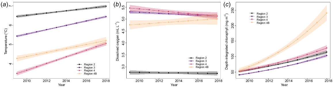
Elevated temperatures corresponding to the marine heat wave of 2014–2016 (Bond et al. 2015; Gentemann et al. 2017) were detected in the data collected in the near-bottom waters of Biological Regions 3 and 4 (Fig. S1), although they were not apparent until 2015. Danielson et al. (2022) found a similar pattern of delayed warming in continental shelf bottom waters during this marine heat wave. Maximum temperatures in those regions decreased notably in the following years, whereas minimum temperatures had small increases (Region 4) or smaller decreases (Region 3), resulting in higher mean temperatures.
Mean station DO ranged from 0.7 to 7.6 mL L−1 coast wide (Fig. 5b). The best-fitting linear model for DO included a year by region interaction (Table 4b), although the AIC difference between this model and the one without an interaction was relatively small. Thus, there was some evidence for regional differences in DO trends over the 10-year study period. Fig. 6b, showing model predictions for DO, shows slightly declining mean DO for Regions 3 and 4, whereas DO increases somewhat, on average, (with high uncertainty) for Region 4B. Region 2 had notably lower DO than did the other three regions (Table 2, Fig. 6b, S3), and additionally, hypoxia was found at both shallow and deep stations in Region 2, but only at deep stations in the other areas (Table 3).
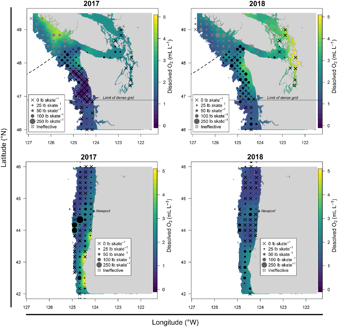
Fig. 7 shows maps of DO off the western coast of USA, with the original data being smoothed using a simple exponential geostatistical model (Cressie 1993) so as to make the DO data easier to interpret visually. (Our intention is to visually highlight the hypoxic event in 2017 and therefore the exact choice of smoother is not important.) In 2017, a large cluster of stations had near-bottom DO at or below the Pacific halibut minimum threshold of 0.9 mL L−1 (Sadorus et al. 2014) detected during the FISS. Pacific halibut was not captured at stations within the threshold outline, whereas in other years there were moderate densities within this region. In 2018, low concentrations of DO were also observed over a wide area further south of the 2017 occurrence. However, the affected zone typically had low Pacific halibut catch rates even in years when hypoxia was not present, and the hypoxic stations were interspersed with stations above the minimum DO threshold. The indication was that hypoxia did not have a notable distributional impact in 2018, as it did in 2017.
Estimated near-bottom dissolved oxygen concentration (DO, mL L−1) off the western coast of USA in 2017 (left panel) and 2018 (right panel) with Pacific halibut weight-per-unit-catch effort values from the IPHC FISS overlaid with black symbols. Stations with DO of ≤0.9 mL L−1 are outlined in white. Weight categories per skate are 25 lb (~11.3 kg), 50 lb (~22.7 kg), 100 lb (~45.4 kg) and 250 lb (~113.4 kg).
Coast-wide mean station near-bottom salinity ranged from 30.8 to 34.1. Biological Region 2 had the highest mean salinity and Region 3 had the lowest (Table 2, Fig. 5c, S3). In Region 2, stations with higher mean salinity were both offshore and inshore, with the southern stations somewhat uniform and high relative to stations further to the north that displayed increasing spatial variability. Region 3 stations that had higher mean salinity tended to be offshore and lower-salinity stations tended to be nearshore. In Region 4, lower-salinity stations were located near-shore in the Gulf of Alaska and around the Pribilof Islands and St Matthew Island in the Bering Sea. Higher-salinity stations were located further offshore at deeper depths and along the Bering Sea shelf edge. Region 4B stations tended to have salinity in the higher end of the range seen coast-wide, with minimal variability. Owing to its bimodal distribution, salinity data were not conducive to linear modelling, but overall salinity values were consistent over the 10-year time span, with no noteworthy temporal trending.
Mean station depth-integrated chlorophyll-a concentration ranged from 20.3 to 409.8 mg m−2. The coast-wide average over the 10-year time span was 99.60 mg m−2 (Table 2). There was high variability both spatially and temporally across the geographical range (Fig. 5d, S4). On average, chlorophyll-a concentrations increased over time across all regions, but with strong evidence that rates of increase varied spatially (Table 4c). The plot of back-transformed predicted means (Fig. 6c) showed that estimated rates of increases were much higher in Biological Region 4B than other regions, which had similar rates of increase.
Spatio-temporal modelling using environmental covariates
The fitted model with the lowest DIC included DO, but not temperature (Model G), with DO modelled as a quadratic function with separate intercept parameters when DO is less than 0.9 mL L−1 (DIC = 9887.9, Table 5). The model without the additional DO intercept parameters (Model F) was only a slightly poorer fit, with DIC = 9888.3. Although a model with bottom temperature on its own provided a somewhat better fit than did the base model (DIC = 9957.8 for quadratic Model C v. 9961.6, Table 5), much greater improvements in the DIC were obtained by adding DO and removing temperature. Almost all temperature measurements were within the range typically encountered by Pacific halibut (98% of values were between 4 and 10°C; see Sadorus et al. 2014 for a review of temperature-range studies), and it seems likely that any apparent improvement in model fit when adding bottom temperature to the base model was a result of the strong correlation with DO (Fig. 3). Whereas all parameter estimates for bottom temperature had relatively large standard deviations and were greatly affected by the addition of DO to the model (even changing sign in Model E; Table 5), DO parameters have low standard deviations relative to the mean and were much less affected by whether temperature was included in the model or not. The k-fold cross-validation MSE values selected the same model as did the DIC, but ranked models including temperature more poorly than those that omitted this covariate.
| Model | Parameter estimates | DIC | ΔDIC | MSE k | ||||||||||
|---|---|---|---|---|---|---|---|---|---|---|---|---|---|---|
| Zero model component x(s,t) | Non-zero model component y(s,t) | |||||||||||||
| Temperature | DO | Temperature | DO | |||||||||||
| β x1 | β x2 | β x3 | β x4 | β x5 | β y1 | β y2 | β y3 | β y4 | β y5 | |||||
| A (base) | 9961.6 | 73.7 | 2413 | |||||||||||
| B | −0.181 (0.135) | 0.162 (0.034) | 9960.3 | 72.4 | 2428 | |||||||||
| C | 1.847 (0.871) | −0.115 (0.050) | 0.953 (0.463) | −0.047 (0.028) | 9957.8 | 69.9 | 2431 | |||||||
| D | 1.365 (0.929) | −0.122 (0.055) | 0.652 (0.145) | 0.734 (0.471) | −0.052 (0.029) | 0.356 (0.070) | 9931.6 | 43.7 | 2450 | |||||
| E | −1.481 (0.945) | 0.044 (0.054) | 2.857 (0.038) | −0.337 (0.051) | −1.017 (0.604) | 0.057 (0.038) | 1.258 (0.194) | −0.144 (0.031) | 9896.6 | 8.7 | 2452 | |||
| F | 2.454 (0.335) | −0.328 (0.050) | 1.040 (0.149) | −0.115 (0.022) | 9888.3 | 0.4 | 2389 | |||||||
| G | 1.973 (0.367) | −0.267 (0.052) | −1.491 (0.517) | 0.948 (0.152) | −0.105 (0.023) | −0.892 (0.358) | 9887.9 | 0.0 | 2380 | |||||
Relative model fit is compared using the deviance information criterion (DIC), and the MSEk from the k-fold cross-validation. Lower values imply a better model fit. ΔDIC is the difference between a model’s DIC and that of the best-fitting model. Parameter estimates (posterior means) of covariate coefficients for temperature and DO (with posterior standard deviations in parentheses below) are shown for each model.
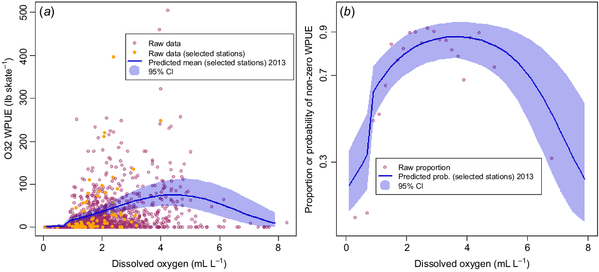
Fig. 8 plots the observed WPUE data against DO, together with posterior predicted means of the 10 selected prediction stations (and 95% posterior credible intervals) for Model F. Although Model F had almost the same DIC as did the best-fitting model, it appears that a simple quadratic model over the whole range of DO values does not capture the drop to near-zero WPUE as DO decreases below 0.9 mL L−1 (Fig. 8a). Likewise, when considering only the binary zero or non-zero model component (x(s,t)) in Fig. 8b, mean posterior predicted values of the probability of non-zero WPUE for the selected stations are much higher than the raw observed proportions (as calculated over all stations and years). Note that each point in Fig. 8b and 9b represents a proportion calculated from between 19 and 131 observations of zeros and non-zeros.
Comparison of model predictions (Model F) with raw data. (a) O32 WPUE plotted against DO, with points indicating raw observed data, and the line showing predicted values for the selected prediction stations (see text, Fig. 3), with 95% posterior credible intervals (shaded region). (b) Raw proportions of non-zero WPUE values from all stations in all years for binned DO values (points) and posterior model predictions of the probability of non-zero WPUE for the selected prediction stations in 2013 (solid line), with 95% posterior credible intervals (shaded region). Note that each raw proportion in (b) was computed from at least 19 and up to 131 binned observations. WPUE conversion: 1 lb = ~0.45 kg.

Comparison of model predictions (Model G) with raw data. (a) O32 WPUE plotted against DO, with points indicating raw observed data, and the line showing predicted values for the selected stations (see text, Fig. 3), with 95% posterior credible intervals (shaded region). (b) Raw proportions of non-zero WPUE values from all stations in all years for binned DO values (points) and posterior model predictions of the probability of non-zero WPUE for the selected stations in 2013 (solid line), with 95% posterior credible intervals (shaded region). Note that each raw proportion in (b) was computed from at least 19 and up to 131 binned observations. WPUE conversion: 1 lb = ~0.45 kg.
Model G, with separate intercept parameter for data with DO < 0.9 mL L−1, does a little better at predicting the low probability of non-zero WPUE for very low DO (Fig. 9b); however, when considering WPUE overall (Fig. 9a), predictions are very close to the near-zero observed WPUE values associated with a very low DO. That this model had almost the same DIC as Model F is presumably due to the relatively low number of observations with DO < 0.9 mL L−1, only 5% of the values used in this modelling. Overall, the quadratic shape of the prediction curves appears to characterise observed patterns in the data quite well. However, we note that we lack a physiological explanation for decreased Pacific halibut density at high values of DO. This highlights the need for more data at both high and low concentrations of DO, so as to provide more confidence in our understanding of the relationship at both ends of the range of DO values.
Discussion
Modelling of future environmental conditions under climate-change scenarios indicates that ocean temperatures will increase overall (Holsman et al. 2018), as they have done in the period from 1950 to 2009 (Poloczanska et al. 2016), and recent studies have correlated marine species distribution shifts, particularly northward, with changes in temperature (e.g. Pinsky et al. 2013; Morley et al. 2018). Species in the northern Pacific are expected to shift poleward (Cheung et al. 2015) as minimum temperature barriers are breached in the north and maximum temperature barriers shift northward in the south. Pacific halibut is routinely found across a relatively wide depth range (down to 500 m in summer and deeper in winter) and latitudinal (Fig. 1) ranges. During the 10-year period of this study, Pacific halibut was caught during the FISS in temperatures ranging from just below 0°C to just over 13°C, with the median number of fish being caught mid-range between 5 and 6°C. This range generally agrees with other studies where adult Pacific halibut was found to occupy temperatures up to 13.6°C and as low as 1.4°C, with the middle of the range being the most populated (Best 1977; Loher and Seitz 2006; Seitz et al. 2007, 2008; Loher and Blood 2009). As waters warm and possibly exceed the normal range, temperature-related distribution changes in the future for Pacific halibut may include poleward expansion or expansion to deeper depths, driven by a need to maintain consistent temperature in juveniles and adults, or a geographic shift in spawning ground success (Smith et al. 2019).
DO concentration in the eastern North Pacific Ocean has been declining since 1980 (Booth et al. 2014), and the bottom depth at which hypoxia is detected may be relevant to demersal species because deep water is more often naturally low in DO and this feature tends to be more spatially permanent (Palmier and Ruiz-Pino 2009) than in more shallow water. Pacific halibut have routinely been found at depths of up to 500 m and, as such, may be somewhat adapted to hypoxia at deeper depths. Conversely, shallow-water hypoxia on the continental shelf is often caused by episodic external inputs to the system, which promote particularly intense phytoplankton blooms leading to significant microbial respiration. These external inputs can include nutrient run-off as seen in the Gulf of Mexico (Rabalais et al. 2002) or upwelling of low-oxygen water in eastern boundary currents (e.g. Grantham et al. 2004). In Biological Region 2, upwelling-driven seasonal hypoxia has been documented periodically throughout the historical record on the outer continental shelf of Oregon and Washington (Connolly et al. 2010). Beginning in 2002, episodic hypoxia has been documented as a periodic feature of the inner shelf (Chan et al. 2008) off the USA western coast, and in these cases, can form in a matter of days (Connolly et al. 2010), displacing predators and mobile prey, and causing mortality of more slow-moving and sessile organisms. Pacific halibut has a minimum DO threshold of 0.9 mL L−1 (Sadorus et al. 2014), a value periodically reached or exceeded in Region 2 in both shallow and deeper stations as a result of the episodic upwelling in this region. The mean near-bottom DO at a given location may be relevant to its impact on species in the area. Biological Region 2 near-bottom stations are routinely lower in DO than are most of the stations in the other regions (Fig. 5b), making Region 2 particularly susceptible to hypoxic conditions in the presence of additional factors that may shift oxygen concentrations progressively lower. Even though the other biological regions indicated statistical differences in DO concentration, the magnitude of the differences may not be biologically important to Pacific halibut when DO exceeds hypoxic concentrations (hypoxia defined as ≤1.4 mL L−1; Diaz and Rosenburg 1995), as was the case in Regions 3, 4 and 4B.
The pattern of salinity in Biological Region 2, i.e. uniformly higher-salinity stations to the south and lower-salinity stations with higher variability to the north (Fig. 5c), reflects the influences of the two current systems contained in the area (Talley 2002) and the upwelling nature of the region. The near-bottom salinity at stations in Regions 3 and 4 displays a pattern of fresher water nearshore, where depths tend to be more shallow and freshwater runoff is likely to influence water chemistry, compared with more saline waters that exist at offshore stations and at greater depths. The pattern of salinity in Region 4B is not similar to those of the other regions. Salinity may be relevant to survival and advection of Pacific halibut eggs and larvae (Forrester and Alderdice 1973; Riis-Vestergaard 1982); however, it remains unclear how changes in salinity may affect demersal-stage fish and further study is needed.
The effect of changes in water column chlorophyll-a concentration on Pacific halibut has not been determined, nor is the connection clear more generally between primary production and predators that occupy higher trophic levels (e.g. Grémillet et al. 2008; Friedland et al. 2012). There was evidence of changes over time in the 10-year profiler time series, and it may be that chlorophyll-a concentration changes disrupt food-web structure in the lower trophic levels, which can lead to disruptions of upper trophic levels occupied by Pacific halibut, but that hypothesis has not been investigated. Providing a baseline for these measurements here may benefit future research in this area.
An objective of this analysis was to qualitatively assess whether biological regions, designed as management tools to preserve bio-complexity (Hicks and Stewart 2018), also reflect reasonable geographic groupings based on environmental conditions. Although some overlap of the environmental factors measured in this study exists, these areas appear to be a reasonable way of grouping the Pacific halibut North American habitat from an environmental perspective. In addition to the factors measured for this study, other environmental differences among regions may further contribute to the distinctions, including bathymetric complexity and food-web variations (Aydin et al. 2007), as well as differences in circulation systems (Stabeno et al. 2004; Henson and Thomas 2008; Checklay and Barth 2009). Aligning the biological and environmental datasets expands the quantity and type of information available for Pacific halibut stock assessment by allowing environmental co-variates at both a local and regional level.
As an example, mapped DO data, together with the results of the spatio-temporal modelling exercise in IPHC Regulatory Area 2A, helped identify an environmental cause for a major distribution shift observed during the IPHC FISS. In this case, model results confirmed that there was strong evidence that Pacific halibut density indices were dependent on the DO covariate, but there was no clear evidence for a relationship between density and bottom temperature in this region where extremes in bottom temperatures are relatively uncommon. We note that Essington et al. (2022) also selected a model with a cutoff term for DO and without temperature when modelling sablefish data in the same region. The DO example in the current work demonstrates how spatio-temporal modelling can aid in the interpretation of observed patterns of spatial variation in density, potentially supporting management decisions that depend on a clear understanding of what is driving distributional change.
We note that other authors have argued for alternative parameterisations of the type of spatial model used in our work (Thorson 2018) but a model structure with a presence–absence component, x(s,t), was preferred here, so as to more easily characterise factors affecting the presence or absence of Pacific halibut in survey sets. At present, inclusion of environmental covariates in models of Pacific halibut data remains at the exploratory stage as we seek to understand its utility for species management, and future work will no doubt lead to further refinement of the models.
As has been noted previously (Webster et al. 2020), some care must be taken in interpreting catch-rate indices and resulting analytical output, as such indices depend on both density and catchability of fish. The IPHC attempts to control factors affecting the latter by using a highly standardised survey design, including standardised gear and the size and quality of bait. The IPHC also applies an adjustment for competition for baits (Clark 2008) that attempts to account for an important component of spatial and temporal variation in catch probability of individual fish. Nevertheless, the current data and modelling approaches cannot parse out the effects of environmental covariates on density from those on catchability, and results must be interpreted with some caution for this reason.
A decade of annual data collection has allowed for the description of baseline conditions in an era when these conditions are expected to alter in the future owing to global climate change (Intergovernmental Panel on Climate Change 2018). In fact, the warming trend detected in this decade of profiler data reflects a larger trend of warming that is currently being realised on a global scale. DO in the global ocean is projected to continue to decline (Breitburg et al. 2018) and waters are expected to freshen at higher latitudes (Oka et al. 2017), although neither the DO nor the salinity datasets examined here displayed notable trends. Primary production is inherently variable and is projected to increase in the Bering Sea and experience a 10–20% decrease in the Northeast Pacific Ocean (Holsman et al. 2018). Related to these changes is a projected increase of extreme episodic events (Oliver et al. 2018) such as marine heat waves, such as the one experienced in the northern Pacific beginning in 2014 (Bond et al. 2015). Changing conditions at deeper depths may be delayed compared with the surface ocean, such that demersal species may experience environmental changes differently from pelagic-dwelling species (Amaya et al. 2023), making a baseline near-bottom dataset particularly relevant to both the Pacific halibut stock assessment as well as those involving other demersal continental shelf species in the northern Pacific.
Data availability
Water column profiler data used in this article are available from the International Pacific Halibut Commission website: https://www.iphc.int/datatest/data/water-column-profiler-data.
Declaration of funding
Profiler project funding came from NOAA Grant NA08NMF4720648, Oregon Department of Fish and Wildlife Restoration and Enhancement Grant #54008 945132-09, and IPHC contracting party appropriations.
Acknowledgements
We extend our gratitude to the vessel crews and biologists who collected these data over the years. We thank the two anonymous reviewers who helped improve this paper for publication. Thank you to Joan Forsberg (IPHC), Colin Jones (IPHC) and Dr Carol Ladd (NOAA) for their earlier reviews of the manuscript, and to Tom Kong for assistance with figures. This is CICOES (formerly JISAO) contribution 2020-1112, NOAA/EcoFOCI contribution EcoFOCI-0958, NOAA/PMEL contribution 5183, and IPHC contribution IPHC-2023-MS003.
References
Amaya DJ, Jacox MG, Alexander MA, Scott JD, Deser C, Capotondi A, Phillips AS (2023) Bottom marine heatwaves along the continental shelves of North America. Nature Communications 14, 1038.
| Crossref | Google Scholar | PubMed |
Bitetto I, Romagnoni G, Adamidou A, Certain G, Di Lorenzo M, Donnaloia M, Lembo G, Maiorano P, Milisenda G, Musumeci C, Ordines F, Pesci P, Peristeraki P, Pesic A, Sartor P, Spedicato MT (2019) Modelling spatio-temporal patterns of fish community size structure across the northern Mediterranean Sea: an analysis combining MEDITS survey data with environmental and anthropogenic drivers. Scientia Marina 83(S1), 141.
| Crossref | Google Scholar |
Bond NA, Cronin MF, Freeland H, Mantua N (2015) Causes and impacts of the 2014 warm anomaly in the NE Pacific. Geophysical Research Letters 42, 3414-3420.
| Crossref | Google Scholar |
Booth JAT, Woodson CB, Sutula M, Micheli F, Weisberg SB, Bograd SJ, Steele A, Schoen J, Crowder LB (2014) Patterns and potential drivers of declining oxygen content along the southern California coast. Limnology and Oceanography 59(4), 1127-1138.
| Crossref | Google Scholar |
Boudreau SA, Shackell NL, Carson S, den Heyer CE (2017) Connectivity, persistence, and loss of high abundance areas of a recovering marine fish population in the Northwest Atlantic Ocean. Ecology and Evolution 2017, 9739-9749.
| Crossref | Google Scholar |
Breitburg D, Levin LA, Oschlies A, Grégoire M, Chavez FP, Conley DJ, Garçon V, Gilbert D, Gutiérrez D, Isensee K, Jacinto GS, Limburg KE, Montes I, Naqvi SWA, Pitcher GC, Rabalais NN, Roman MR, Rose KA, Seibel BA, Telszewski M, Yasuhara M, Zhang J (2018) Declining oxygen in the global ocean and coastal waters. Science 359(6371), eaam7240.
| Crossref | Google Scholar |
Cameletti M, Lindgren F, Simpson D, Rue H (2013) Spatio-temporal modeling of particulate matter concentration through the SPDE approach. AStA Advances in Statistical Analysis 97, 109-131.
| Crossref | Google Scholar |
Chan F, Barth JA, Lubchenco J, Kirincich A, Weeks H, Peterson WT, Menge BA (2008) Emergence of anoxia in the California current large marine ecosystem. Science 319, 920.
| Crossref | Google Scholar | PubMed |
Checklay DM, Jr., Barth JA (2009) Patterns and processes in the California Current system. Progress in Oceanography 83(1–4), 29-64.
| Crossref | Google Scholar |
Cheung WWL, Brodeur RD, Okey TA, Pauly D (2015) Projecting future changes in distributions of pelagic fish species of Northeast Pacific shelf seas. Progress in Oceanography 130, 19-31.
| Crossref | Google Scholar |
Connolly TP, Hickey BM, Geier SL, Cochlan WP (2010) Processes influencing seasonal hypoxia in the northern California Current System. Journal of Geophysical Research 115, C03021.
| Crossref | Google Scholar | PubMed |
Danielson SL, Hennon TD, Monson DH, Suryan RM, Campbell RW, Baird SJ, Holdereid K, Weingartner TJ (2022) Temperature variations in the northern Gulf of Alaska across synoptic to century-long time scales. Deep-Sea Research – II. Topical studies in Oceanography 203, 105155.
| Crossref | Google Scholar |
Diaz RJ (2002) Hypoxia and anoxia as global phenomena. In ‘Fish Physiology, Toxicology, and Water Quality: Proceedings of the Sixth International Symposium, Fish Physiology, Toxicology, and Water Quality’, 22–26 January 2001, La Paz, BCS, Mexico. (Ed. RV Thurston) pp. 183–202. (US Environmental Protection Agency, Ecosystems Research Division: Atlanta, GA, USA)
Diaz RJ, Rosenburg R (1995) Marine benthic hypozia: a review of its ecological effets and the behavioural responses of benthic macrofauna. Oceanography and Marine Biology: An Annual Review 33, 245-303.
| Google Scholar |
Dunbabin M, Marques L (2012) Robots for environmental monitoring: Significant advancements and applications. IEEE Robotics & Automation Magazine 19(1), 24-39.
| Crossref | Google Scholar |
Essington TE, Anderson SC, Barnett LAK, Berger HM, Siedlecki SA, Ward EJ (2022) Advancing statistical models to reveal the effect of dissolved oxygen on the spatial distribution of marine taxa using thresholds and a physiologically based index. Ecography 2022, e06249.
| Crossref | Google Scholar |
Friedland KD, Stock C, Drinkwater KF, Link JS, Leaf RT, Shank BV, Rose JM, Pilskaln CH, Fogarty MJ (2012) Pathways between primary production and fisheries yields of large marine ecosystems. PLoS ONE 7(1), e28945.
| Crossref | Google Scholar | PubMed |
Gentemann CL, Fewings MR, García-Reyes M (2017) Satellite sea surface temperatures along the West Coast of the United States during the 2014–2016 northeast Pacific marine heat wave. Geophysical Research Letters 44(1), 312-319.
| Crossref | Google Scholar |
Grantham BA, Chan F, Nielsen KJ, Fox DS, Barth JA, Huyer A, Lubchenco J, Menge BA (2004) Upwelling-driven nearshore hypoxia signals ecosystem and oceanographic changes in the northeast Pacific. Nature 429(6993), 749-754.
| Crossref | Google Scholar | PubMed |
Grémillet D, Lewis S, Drapeau L, van Der Lingen CD, Huggett JA, Coetzee JC, Verheye HM, Daunt F, Wanless S, Ryan PG (2008) Spatial match–mismatch in the Benguela upwelling zone: should we expect chlorophyll and sea-surface temperature to predict marine predator distributions? Journal of Applied Ecology 45(2), 610-621.
| Crossref | Google Scholar |
Henson SA, Thomas AC (2008) A census of oceanic anticyclonic eddies in the Gulf of Alaska. Deep-Sea Research – I. Oceanographic Research Papers 55, 163-176.
| Crossref | Google Scholar |
Hilborn R, Quinn TP, Schindler DE, Rogers DE (2003) Biocomplexity and fisheries sustainability. Proceedings of the National Academy of Sciences of the United States of America 100, 6564-6568.
| Crossref | Google Scholar |
Holsman K, Hollowed A, Ito S, Bograd S, Hazen E, King J, Mueter F, Perry RI (2018) Chapter 6: Climate change impacts, vulnerabilities and adaptations: North Pacific and Pacific Arctic marine fisheries. In ‘Impacts of climate change on fisheries and aquaculture’. FAO Fisheries and Aquaculture Technical Paper 627. (Eds M Barange, T Bahri, MCM Beveridge, KL Cochrange, S Funge-Smith, F Poulain) pp. 113–138. (Food and Agriculture Organization of the United Nations).
Ibaibarriaga L, Uriarte A, Laconcha U, Bernal M, Santos M, Chifflet M, Irigoien X (2013) Modelling the spatio-temporal distribution of age-1 Bay of Biscay anchovy (Engraulis encrasicolus) at spawning time. Scientia Marina 77(3), 461-472.
| Crossref | Google Scholar |
Intergovernmental Panel on Climate Change (2018) Summary for Policymakers. In ‘Global Warming of 1.5°C. An IPCC Special Report on the impacts of global warming of 1.5°C above pre-industrial levels and related global greenhouse gas emission pathways, in the context of strengthening the global response to the threat of climate change, sustainable development, and efforts to eradicate poverty’. (Eds V Masson-Delmotte, P Zhai, H-O Pörtner, D Roberts, J Skea, PR Shukla, A Pirani, W Moufouma-Okia, C Péan, R Pidcock, S Connors, JBR Matthews, Y Chen, X Zhou, MI Gomis, E Lonnoy, T Maycock, M Tignor, T Waterfield) pp. 1–24. (Cambridge University Press) 10.1017/9781009157940.001
International Pacific Halibut Commission (2020) The Fishery-Independent Setline Survey (FISS). (IPHC, Seattle, WA, USA) Available at https://www.iphc.int/management/science-and-research/fishery-independent-setline-survey-fiss
Keller AA, Ciannelli L, Wakefield WW, Simon V, Barth JA, Pierce SD (2017) Species-specific responses of demersal fishes to near-bottom oxygen levels within the California Current large marine ecosystem. Marine Ecology Progress Series 568, 151-173.
| Crossref | Google Scholar |
Koenigstein S, Mark FC, Gößling-Resemann S, Rueter H, Poertner H-O (2016) Modelling climate change impacts on marine fish populations: process-based integration of ocean warming, acidification, and other environmental drivers. Fish and Fisheries 17(4), 972-1004.
| Crossref | Google Scholar |
Lindgren F, Rue H (2015) Bayesian spatial modelling with R-INLA. Journal of Statistical Software 63, 1-27.
| Crossref | Google Scholar |
Link JS, Marshak AR (2019) Characterizing and comparing marine fisheries ecosystems in the United States: determinants of success in moving toward ecosystem-based fisheries management. Reviews in Fish Biology and Fisheries 29, 23-70.
| Crossref | Google Scholar |
Loher T, Blood CA (2009) Seasonal dispersion of Pacific halibut (Hippoglossus stenolepis) summering off British Columbia and the US Pacific Northwest evaluated via satellite archival tagging. Canadian Journal of Fisheries and Aquatic Sciences 66, 1409-1422.
| Crossref | Google Scholar |
Loher T, Seitz AC (2006) Seasonal migration and environmental conditions of Pacific halibut Hippoglossus stenolepis, elucidated from pop-up archival transmitting (PAT) tags. Marine Ecology Progress Series 317, 259-271.
| Crossref | Google Scholar |
Morley JW, Selden RL, Latour RJ, Frolicher TL, Seagraves RJ, Pinsky ML (2018) Projecting shifts in thermal habitat for 686 species on the North American continental shelf. PLoS ONE 13(5), e0196127.
| Crossref | Google Scholar | PubMed |
National Oceanic and Atmospheric Administration (2022) Alaska Groundfish Bottom Trawl Survey Data. (NOAA) Available at https://www.fisheries.noaa.gov/alaska/commercial-fishing/alaska-groundfish-bottom-trawl-survey-data#additional-resources
National Oceanic and Atmospheric Administration, Pacific Marine Environmental Laboratory (2023) Mooring Site Locations 1991–2016: Bering Sea, Aleutian Islands, Gulf of Alaska. Revised: 22 November 2023. (NOAA, PMEL: Seattle, WA, USA) Available at https://www.pmel.noaa.gov/foci/foci_moorings/mooring_info/mooring_location_info.html
Oka E, Katsura S, Inoue H, Kojima A, Kitamoto M, Nakano T, Suga T (2017) Long-term change and variation of salinity in the western North Pacific subtropical gyre revealed by 50-year long observations along 137°E. Journal of Oceanography 73(4), 479-490.
| Crossref | Google Scholar |
Oliver ECJ, Perkins-Kirkpatrick SE, Holbrook JJ, Bindoff NI (2018) Anthropogenic and natural influences on record 2016 marine heatwaves. In ‘Explaining extreme events of 2016 from a climate perspective. Special supplement to the Bulletin of the American Meterorological Society’. Vol. 99(1). (Eds SC Herring, N Christidis, A Howell, JP Kossin, CJ Schreck III, PA Stott) pp. S44–S49. 10.1175/BAMS-D-17-0093.1
Palmier A, Ruiz-Pino D (2009) Oxygen minimum zones (OMZs) in the modern ocean. Progress in oceanography 80(3–4), 113-128.
| Crossref | Google Scholar |
Pinsky ML, Worm B, Fogarty MJ, Sarmiento JL, Levin SA (2013) Marine taxa track local climate velocities. Science 341, 1239-1242.
| Crossref | Google Scholar | PubMed |
Poloczanska ES, Burrows MT, Brown CJ, Molinos JG, Halpern BX, Hoegh-Guldberg O, Kappel CV, Moore PJ, Richardson AJ, Schoerman DS, Sydeman WJ (2016) Responses of marine organisms to climate change across oceans. Frontiers in Marine Science 3, 62.
| Crossref | Google Scholar |
Rabalais NN, Turner RE, Wiseman WJ Jr (2002) Gulf of Mexico hypoxia, a.k.a. ‘The Dead Zone’. Annual Review of Ecology and Systematics 33(1), 235-263.
| Crossref | Google Scholar |
Riis-Vestergaard J (1982) Water and salt balance of halibut eggs and larvae (Hippoglossus hippoglossus). Marine Biology 70, 135-139.
| Crossref | Google Scholar |
Sadorus LL, Mantua NJ, Essington T, Hickey B, Hare S (2014) Distribution patterns of Pacific halibut (Hippoglossus stenolepis) in relation to environmental variables along the continental shelf waters of the US West Coast and southern British Columbia. Fisheries Oceanography 23(3), 225-241.
| Crossref | Google Scholar |
Selden R, Pinsky M (2019) Chapter 20 – Climate change adaptation and spatial fisheries management. In ‘Predicting future oceans’. (Eds AM Cisneros-Montemayor, WWL Cheung, Y Ota) pp. 207–214. (Elsevier) 10.1016/B978-0-12-817945-1.00023-X
Shelton AO, Thorson JT, Ward EJ, Feist BE (2014) Spatial semiparametric models improve estimates of species abundance and distribution. Canadian Journal of Fisheries and Aquatic Science 71, 1655–1666. 10.1139/cjfas-2013-0508
Sigler M, Hollowed A, Holsman K, Zador S., Haynie A, Himes-Cornell A, Mundy P, Davis S, Duffy-Anderson J, Gelatt T, Gerke B, Stabeno P (2016) Alaska regional action plan for the southeastern Bering Sea: NOAA fisheries climate science strategy. NOAA Technical Memo NMFS-AFSC-336, NOAA, Alaska Fisheries Science Center. 10.7289/V5/TM-AFSC-336
Smith KA, Dowling CE, Brown J (2019) Simmered then boiled: multi-decadal poleward shift in distribution by a temperature fish accelerates during marine heatwave. Frontiers in Marine Science 6, 407.
| Crossref | Google Scholar |
Spiegelhalter DJ, Best NG, Carlin BP, Van der Linde A (2002) Bayesian measures of model complexity and fit. Journal of the Royal Statistical Society, B 64, 583-639.
| Crossref | Google Scholar |
Stabeno PJ, Bond NA, Hermann AJ, Kachel NB, Mordy CW, Overland JE (2004) Meteorology and oceanography of the northern Gulf of Alaska. Continental Shelf Research 24(7–8), 859-897.
| Crossref | Google Scholar |
Stevenson DE, Lauth RR (2019) Bottom trawl surveys in the northern Bering Sea indicate recent shifts in the distribution of marine species. Polar Biology 42, 407-421.
| Crossref | Google Scholar |
Thorson JT (2018) Three problems with the conventional delta-model for biomass sampling data, and a computationally efficient alternative. Canadian Journal of Fisheries and Aquatic Science 75, 1369-1382.
| Crossref | Google Scholar |
Webster RA, Soderlund E, Dykstra CL, Stewart IJ (2020) Monitoring change in a dynamic environment: spatio-temporal modelling of calibrated data from different types of fisheries surveys of Pacific halibut. Canadian Journal of Fisheries and Aquatic Sciences 77(8), 1421-1432.
| Crossref | Google Scholar |