

Development and application of the Riparian Mapping Tool to identify priority rehabilitation areas for nitrogen removal in the Tully–Murray basin, Queensland, Australia
D. W. Rassam A C and D. Pagendam BA CSIRO Land and Water, 120 Meiers Road, Indooroopilly, Qld 4068, Australia.
B The University of Queensland, St Lucia, Qld 4067, Australia.
C Corresponding author. Email: david.rassam@csiro.au
Marine and Freshwater Research 60(11) 1165-1175 https://doi.org/10.1071/MF08358
Submitted: 22 December 2008 Accepted: 22 May 2009 Published: 17 November 2009
Abstract
One feature of riparian zones is their ability to significantly reduce the nitrogen loads entering streams by removing nitrate from the groundwater. A novel GIS model was used to prioritise riparian rehabilitation in catchments. It is proposed that high-priority areas are those with a high potential for riparian denitrification and have nearby land uses that generate high nitrogen loads. For this purpose, we defined the Rehabilitation Index, which is the product of two other indices, the Nitrate Removal Index and the Nitrate Interception Index. The latter identifies the nitrate contamination potential for each raster cell in the riparian zone by examining the extent and proximity of agricultural urban land uses. The former is estimated using a conceptual model for surface–groundwater interactions in riparian zones associated with middle-order gaining perennial streams, where nitrate is removed via denitrification when the base flow interacts with the carbon-rich riparian sediments before discharging to the streams. Riparian zones that are relatively low in the landscape, have a flat topography, and have soils of medium hydraulic conductivity are most conducive to denitrification. In the present study, the model was implemented in the Tully–Murray basin, Queensland, Australia, to produce priority riparian rehabilitation area maps.
Additional keywords: denitrification, GIS, nitrate, stream aquifer interaction.
Introduction
Recent studies in several parts of Australia have shown nitrogen to be a key nutrient likely to trigger algal blooms and related problems in both coastal waters (e.g. Dennison and Abal 1999) and freshwater bodies (e.g. Mosisch et al. 1999, 2001). Sources of nitrogen that are associated with land use include fertiliser application, soil erosion, inputs from human and animal wastes, and, in some cases, precipitation (e.g. from vehicle emissions in large cities) (Hunter et al. 2006).
Riparian zones can trap sediment and associated nutrients from surface run-off, thus reducing downstream loadings (Prosser et al. 1999). In addition, riparian zones host a variety of subsurface processes that have the potential to transform and remove nitrogen, including via the microbial process of denitrification (Cirmo and McDonnell 1997). Many studies have demonstrated substantial reductions in nitrate as subsurface water passes through riparian buffer zones (e.g. Lowrance et al. 1984; Dosskey 2001) and the role of riparian zones in facilitating denitrification has received particular attention (e.g. Hill 1979; Vidon and Hill 2004). Denitrification is of specific interest because it results in the conversion of nitrate to gaseous forms of nitrogen and is therefore a pathway for the permanent removal of nitrogen from the land/water system. However, the greenhouse gas N2O is emitted during this process; van den Heuvel et al. (2009) stated that riparian buffer zones might be classified as hotspots for N2O emission at a landscape scale.
Nitrate removal in riparian zones requires a well vegetated riparian zone that provides a plentiful source of organic carbon through the soil profile, and a floodplain hydrology that is conducive to denitrification. The importance of riparian zone hydrology in influencing the extent of denitrification has been emphasised in many studies (e.g. Burt et al. 2002; Rassam et al. 2006). The classical conceptual model suggests that groundwater travels laterally and interacts with riparian sediments before discharging to the stream. This conceptual model for denitrification implies that a shallow water table intercepts the carbon-rich root zone, thus providing anoxic conditions. Flow rates should be slow enough to allow sufficient residence time for denitrification to occur. The hydraulic conductivity of the floodplain plays a critical role. Burt et al. (2002) reported that soils of medium hydraulic conductivities are most conducive to denitrification. Rassam (2005) conducted numerical modelling for coupled flow and solute transport and showed that soils with medium conductivities that range from 0.1 to 1 m day–1 are the most conducive to denitrification. Moreover, topography plays a substantial role in determining the hydrological functioning of riparian zones (Devito et al. 2000).
Within the last decade, there has been increased interest in applying catchment hydrological models to determine the likely impacts on water quality from changes in land-use or land-management practices. An extensive range of hydrological models has been developed with different applications in relation to the riparian zone. Inamdar et al. (1999a , 1999b) developed the Riparian Ecosystem Management Model (REMM) to estimate riparian denitrification. Subsequently, the REMM has been coupled with spatial hydrological models, such as The Groundwater Loading Effects of Agricultural Management System (GLEAMS) and The Soil and Water Assessment Tool (SWAT). GLEAMS (Leonard et al. 1987) focuses on surface and subsurface water and chemical movement in a GIS environment (Tucker et al. 2000a , 2000b ), but has been applied only at a farm scale; whereas SWAT (Neitsch et al. 2005) has been developed for hydrological modelling of catchments and predicts the effects of land management changes on water, sediment and agricultural chemical yields. Cerucci and Conrad (2003) undertook a catchment-scale study that coupled SWAT with REMM to identify the optimal locations for planting riparian vegetation under certain financial constraints (i.e. the cost of acquiring land). Burkart et al. (2004) also examined the problem of placing riparian buffer zones to improve water quality. They concluded that topographic and hydrological indices provide useful and easily acquired information on the hydrological variables critical for identifying key locations for well vegetated riparian buffer zones.
The use of digital elevation models (DEMs) for predicting catchment behaviour via what is commonly referred to as a ‘terrain analysis’ has been in use for well over two decades. Moore et al. (1991) provided a good review of the topic, stating that the topography of a catchment has a major impact on the hydrological, geomorphological and biological processes active in the landscape. Hence, simple spatial indices may be adopted for predicting more complex phenomena. Subsequently, several GIS tools have been developed for the purpose of making rapid, broad-scale assessments of catchments. Beven and Kirkby (1979) developed TOPMODEL and introduced the wetness index, which was used to identify the parts of a catchment that might be surface-saturated. McGlynn and Seibert (2003) assessed the capacity of riparian zones to buffer hillslope run-off using a terrain analysis. Other terrain analysis tools, such as MrVbf (Multi-resolution Valley Bottom Flatness) (Gallant and Dowling 2003), have been used to generate indices of valley slope and scale. The index can potentially be used to identify groundwater constrictions and to delineate geomorphic units such as the depositional parts of landscapes. Baker et al. (2001) outlined the MRI-DARCY model, which attempts to predict subsurface discharge to rivers, lakes and wetlands at a scale useful to environmental managers. Although Baker et al. (2001) recognised that aspects of such modelling could be regarded as a ‘gross over-simplification’, we argue that the approach is necessary to make rapid, broad-scale assessments at a large scale.
In the present study, we outline the Riparian Mapping Tool (RMT), a novel GIS technique that can help land managers identify riparian areas of middle-order gaining streams where rehabilitation is likely to be most effective in enhancing denitrification and reducing nitrogen loads. In the present study, riparian rehabilitation refers to new planting and/or the restoration of damaged riparian buffers to enhance the availability of organic carbon and hence maximise denitrification. To optimise the benefits of riparian rehabilitation, we envisage that information from the RMT can be evaluated alongside priorities for achieving other objectives (e.g. stabilising stream banks, improving wildlife habitats), while also taking into account any social and economic requirements. The RMT stems from the Riparian Nitrogen Model (RNM) of Rassam et al. (2005, 2008). The proposed mapping tool encompasses the hydrological and chemical processes that underpin denitrification in a spatially explicit and simple manner, with relatively low data requirements.
We implemented the RMT in the Tully–Murray basin, far-northern Queensland, Australia (fig. 1 in Kroon 2009) and present a map of stream reaches showing where riparian rehabilitation should be targeted to reduce nitrogen loads in this catchment. The Tully–Murray basin is one of 35 basins discharging into the Great Barrier Reef World Heritage Area. Kroon (2009) indicated that high rainfall combined with near-coastal steep topography and extensively fertilised land use on the floodplain provide the potential for erosion and pollutant transport to the receiving waters. Both monitoring and modelling studies have documented high dissolved inorganic nitrogen loads in the basin (Armour et al. 2009; Bainbridge et al. 2009).
Materials and methods
The methodology adopts an index-based approach to prioritise riparian rehabilitation in the catchments. The stream network and the riparian zone are first generated. Nitrate is removed via denitrification as groundwater interacts with the riparian sediments where denitrification activity increases towards the ground surface. The proposed conceptual model for surface–groundwater interaction is used to estimate an index indicating the volume of water interacting with the riparian zone and residence time. A nitrate-generation index is defined based on land use. The outcome of the methodology is an index that indicates priority areas for riparian rehabilitation. The priority areas are defined as those that have maximal nitrate removal capacity and have land uses that generate maximal nitrate loads in their close proximity.
The underlying assumptions that underpin the RMT are that: (1) the riparian zones have a uniform width and run parallel to the stream network; (2) the groundwater table is parallel to the ground surface with a gradient towards the stream (gaining stream); (3) nitrate is removed via denitrification in the saturated part of the root zone with activity decreasing with depth; and (4) temperature effects are ignored, although they can be a limiting factor on the extent of denitrification (Koszelnik et al. 2007). Although the profile of the denitrification potential is assumed to be constant in this study (point 3), each riparian cell would have a different nitrate removal potential because the hydrology is different (i.e. depth to groundwater table, volume of water interacting with the riparian zone and residence time are all different for each riparian cell).
Generating the stream network and riparian zones
The first step in the DEM analysis is the spatial delineation of the stream network and riparian zones. A DEM is typically used to derive rasters of flow direction and flow accumulation (e.g. O’Callaghan and Mark 1984). Rather than generating a stream network from the digital elevation model, as is undertaken in hydrological modelling, a 1 : 50 K vector drainage hydrology stream network was used to identify the precise locations of the waterways (Bruce and Kroon 2006). Using this data set had the added benefit that the widths of the stream channels were taken into account and therefore the positions of the riparian buffers were spatially accurate. Shape files of the 1 : 50 K streams data were obtained, projected to Albers’ equal area projection and converted to raster data sets for use in the RMT.
Nitrate removal potential
Denitrification rates are highly correlated with the concentration of available electron donors in the soil, which is largely associated with plant growth, litter fall and the roots of riparian vegetation. It is assumed that organic carbon levels are maximal at the soil surface and decline with depth (e.g. Hunter et al. 2006). The distribution of the denitrification rate with depth is modelled using an exponential decay function as follows:
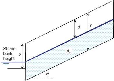
where, referring to Fig. 1, R d (day–1) is the nitrate decay rate (indicating denitrification) at any depth, R max (day–1) is the maximum nitrate decay rate at the soil surface, d is the vertical depth to groundwater measured from the ground surface (m), r is the depth of the root zone (m) and k (m–1) describes the rate at which the denitrification rate declines with depth.
|
As the upper horizons of riparian soils are typically unsaturated for most of the time, the maximum denitrification rate at the soil surface is unlikely to be operable. In contrast, denitrification processes may occur to a small extent below the root zone, but are likely to be negligible. The formulation of Eqn 1 assumes zero denitrification below the rooting depth. Denitrification processes are assumed to be active only in the saturated part of the root zone below the water table (throughout interval r – d; Fig. 2). From Eqn 1, we can derive an average denitrification rate R u throughout the interval r – d (hatched area in Fig. 1) as follows:
|
where R u (day–1) is the average denitrification rate across the saturated root zone. Note that R u = 0 for d ≥ r. The mathematical derivation of Eqn 2 can be found in Rassam et al. (2008).
A first-order decay function is used to calculate nitrate removal with time as a result of denitrification, which is given by:

where t (days) is time, R u is the average denitrification rate through the saturated root zone (defined in Eqn 2) and t μ is the residence time derived from Darcy’s Law; D n varies from 0 to 1 and represents the proportion of nitrate that is removed via denitrification.
The total mass of nitrate that can potentially be removed by the riparian zone is proportional to D n and to the volume of water that passes through the riparian zone (assuming a constant nitrate concentration). Hence, we can define the nitrate removal index η as follows:

where ν represents the volume of water that passes through the riparian zone and is derived from the base-flow index (BFI); this value is normalised so that it ranges from 0 to 1. The BFI is the ratio of base flow to total flow, which is indicative of the volume of water interacting with the riparian zone. In a GIS modelling framework, the nitrate removal index η is obtained by overlaying the two rasters representing denitrification potential and base-flow index. We undertake these calculations for each grid cell in the catchment representing the riparian zone, thus resulting in a spatially explicit index.
Conceptual model for the surface water–groundwater interaction
The surface water and groundwater (SW/GW) interaction is conceptualised as shown in Fig. 2. The water table is considered to be a linear function with a slope equal to that of the ground surface (and therefore also equal to the root zone). The root zone needs to be identified because denitrification occurs during groundwater interaction within its carbon-rich sediments. The saturated part of the root zone (area A s; Fig. 2), which extends across the entire width of the riparian zone, is the active area for denitrification.
Residence time
The residence time needs to be estimated because it dictates the extent of denitrification and is directly proportional to the width of the riparian zone. The residence time, t μ , is derived from the Darcy flux and is given by:
where φ is the inclination angle of the riparian zone, L is the width of the riparian zone, θ is the porosity and K is the hydraulic conductivity of the riparian soil. Residence time is a function of travel distance and flow rate; the latter is in turn a function of the hydraulic conductivity and head gradient.
High nitrate removal as a result of denitrification requires the nitrate-rich groundwater to have an appreciable residence time within the riparian zone. If the flow is too fast (and hence t μ is small), then only a small proportion of the nitrate will be transformed. Conversely, if the flow is too slow, the residence time will be high, but the volume of water (and hence the total amount of nitrate) interacting with the riparian zone will be very low. Therefore, there exists an optimal flow rate that allows a high residence time and at the same time maximises transport through the riparian zone. The ‘optimal hydrology’ for denitrification requires a shallow water table that allows interaction with the most active shallow riparian sediments with an optimal flow rate that allows ample residence time and maximal flows. The optimal flow rate is associated with soils of medium conductivity and ranges from 0.1 to 1 m day–1 (Rassam 2005).
Depth to groundwater table
The proposed model for the SW/GW interaction shown in Fig. 2 is not dynamic; that is, it does not model a variable water-table depth during events. Rather, it assumes a constant (non-event) depth to the water table (d) that is spatially variable depending on landscape attributes. Evaluating the depth to groundwater in a spatial setting is a complex undertaking that is affected by many factors such as geology, hydrology, topography and vegetation.
Rather than relying on deterministic groundwater models that have high data requirements, we used an index-based approach via terrain analysis that can be related to the depth of groundwater. A statistical model with fitting parameters is proposed; those parameters are evaluated through an optimisation process so that the best fit to the observed groundwater levels is achieved. The proposed methodology combines three indices: the MRI-Darcy index of Baker et al. (2001), the wetness index from the TOPMODEL of Beven and Kirkby (1979) and the multi-resolution valley bottom flatness index (MrVbf) of Gallant and Dowling (2003). This proposed three-index model is believed to be superior to that used by Baker et al. (2001), who used the wetness index to predict the depth to the groundwater table.
The MRI-Darcy model treats perennial streams as windows into the groundwater table and uses the elevation of the cells in the stream network grid to extrapolate the shape of the water table in close proximity to a stream (i.e. in the riparian zone). The model uses an inverse distance-weighted estimator for the elevation of the water table in the riparian zone grid cells. The groundwater elevation of the ith grid cell is calculated using:
where E i is the elevation of the phreatic surface for the ith cell in the riparian zone, j is an index for the 10 cells (categorised as part of the stream network) that are nearest to the riparian zone cell, m j is the distance between the riparian cell and the jth stream cell and s j is the elevation of the jth stream cell. The MRI-Darcy index (Di ) for the ith raster cell in the catchment is given by:

where DEM i is the ground surface elevation.
The wetness index of Beven and Kirkby (1979) is calculated as follows:
where W i is the wetness index, tan φ i is the slope of a grid cell, A i is the contributing area for the ith grid cell in the catchment and g is the width of the grid cells.
The multi-resolution valley bottom flatness (MrVbf) of Gallant and Dowling (2003) uses a digital elevation model to identify valley bottoms on the basis of their topographic signature as flat low-lying areas. A key application of the MrVbf index is to provide information for hydrological models at the catchment scale in the form of hydrological units. The index has potential applications in the delineation of hydrological and geomorphic units and for quantitative comparison of catchments.
At each groundwater bore location, the spatial attributes of three topographic indices were obtained. Each of these three indices was obtained from an analysis of 250-m DEMs. Bores that were within a 250-m buffer of a drainage network derived from the 250-m DEM were only retained for the statistical analysis. In total, 23 groundwater bores were used to calibrate the statistical model. The three indices were calculated using The Invisible Modelling Environment of Rahman et al. (2003). A linear model was formulated using the three topographic indices as highly statistically significant predictors of observed groundwater depths. The statistical analysis was conducted using the R statistical software package (www.r-project.org).
Base-flow index
As noted by several previous authors (e.g. Lacey and Grayson 1998; Mazvimavi et al. 2004), base-flow delivery to streams can be a function of a variety of biophysical characteristics. Therefore, we set out to identify significant environmental predictors of base-flow contribution. Several linear statistical models with various fitting parameters were investigated so that the best fit to the observed base-flow indices could be achieved.
Each time series of observed flows was used to calculate the BFI, which was used as the response variable in the linear model. Several potential predictors were tested, including elevation, average long-term rainfall, flow type (unregulated or regulated), average long-term potential evapotranspiration (PET), contributing area, soil hydraulic conductivity, soil porosity, MrVbf index and wetness index. All statistical analyses were carried out in the R statistical environment.
Gauging station data were collated for the Tully–Murray basin as well as for the neighbouring coastal catchments (i.e. the Johnstone and Herbert River catchments). For each geographical location where data had been collected, the entire daily time series was passed through a Lyne–Hollick digital filter (Lyne and Hollick 1979) for the purpose of base-flow separation (with the filtering parameter α set to the default value of 0.925). Other field-based approaches for estimating base flow that include hydrogeological studies and stable isotope characterisation may be used, but their usefulness is limited by their high data requirements.
Nitrate generation and nitrate interception potential
Nitrate sources include the application of N fertilisers, mismanagement of irrigated crops, the disposal of livestock waste (Hallberg 1989) and the cultivation of virgin land (e.g. Ronen et al. 1983; Faillat 1990). We used a simple nitrate generation model where the concentrations varied linearly with land use. The nitrate generation model uses a mean ‘Dry Weather Concentration’ (DWC) of nitrate that is generated for a particular land use, where the DWC refers to the contaminant concentration associated with the base-flow component of the flow. This approach has been used for several catchment models created for south-eastern Queensland (Chiew et al. 2002; Searle 2005).
The nitrate interception potential is calculated by examining the neighbourhood of cells within a specified radius (the neighbourhood disc) surrounding each of the i cells in the riparian zone within a prescribed radius z max. It is calculated according to the following procedure:
-
Identify all of the i cells adjacent to the stream network that are considered to be part of the riparian buffer zone.
-
For each of the i cells, identify the neighbourhood disc, that is, all of the cells within a distance (z max) of the ith riparian cell (focal cell).
-
For each of the i neighbourhood discs, define the set of doubles, S i = {(DWC 1i , z 1i ), (DWC 2i , z 2i ), …, (DWC ni , z ni )}, where each of the cells in the neighbourhood disc has a greater elevation than (and can therefore deliver groundwater to) the focal cell. Here, the DWC ji is the dry-weather nitrate concentration of the jth cell in the ith neighbourhood disc and z ji is the Euclidean distance between the focal riparian cell and the jth cell within the neighbourhood disc.
-
For each of the i neighbourhood discs, use the doubles (DWC ji , z ji ) within set S i to calculate the nitrate interception potential (NIP) of the ith riparian zone cell as:
-
Once the NIP has been calculated for all (i) of the riparian grid cells, normalise the values so that they all fall between 0 and 1 by dividing them by the maximum value of NIP.
The suitability of this methodology was verified by Rassam et al. (2008) in the Maroochy catchment, south-eastern Queensland, Australia. They observed a linear correlation between the NIP and the observed nitrate concentrations in the catchment, which validates its suitability as a predictor of the physical processes governing nitrate generation and interception.
Riparian rehabilitation potential
From the above, the spatial data sets corresponding to η and NIP were then combined to form an aggregated index, the ‘Rehabilitation Potential’. Both η and NIP have values between 0 and 1. The aggregated index, R i , is defined as:

where R i is the ‘Rehabilitation Potential’ for the ith grid cell, which provides a measure of a riparian zone’s ability to intercept subsurface nitrate and successfully remove it via denitrification. The grid of the rehabilitation potential is reclassified into 10 distinct integer classes labelled 1, …, 10. These classes are assigned on the basis of percentiles so that the grid cells in R i with values less than or equal to the 10th percentile are assigned a 1, cells greater than the 10th percentile, but less than the 20th percentile are assigned a 2, and so forth.
Input data sets
A DEM of 25-m cell resolution was used to calculate the slope of the riparian zones. Subsoil hydraulic conductivity was obtained from the Soil Hydrological Properties of Australia (SHPA) data set, which, along with the slope, was used to calculate residence time. Groundwater data for the Tully–Murray system and for neighbouring coastal catchments (i.e. Johnstone and Herbert) were obtained from the groundwater database managed by the Queensland Department of Natural Resources and Water. The data obtained from 23 bore holes were used to calibrate the model for predicting depth to groundwater table.
Gauging station data were collated from 24 sites in the Tully–Murray and neighbouring coastal catchments (i.e. the Johnstone and Herbert River catchments). For each geographical location where data had been collected, the entire daily time series was passed through a Lyne–Hollick digital filter (Lyne and Hollick 1979) for the purpose of base-flow separation. These data sets were used to calibrate the model that predicts the BFI.
For each raster cell in the riparian zone, the RMT estimates an average denitrification rate on the basis of the predicted depth to groundwater table. The three parameters governing the decline in denitrification rates with depth (Eqn 1) are R max = 0.58 day–1, k = 1.16 m–1 and r = 5 m. These parameters were based on experimental estimates of the denitrification rates from south-eastern Queensland outlined in Rassam et al. (2005).
Draft Queensland Land Use Mapping (QLUMP) shape files were obtained from the Queensland Department of Natural Resources and Water. Land use in the catchment was grouped into five categories, with corresponding contamination indices as follows: (1) water = 0.0; (2) urban = 0.375; (3) vegetated = 0.20; (4) grazing = 0.675; and (5) agriculture = 1.0. The values chosen were based on normalised DWCs obtained from the study conducted by Chiew et al. (2002). The concentrations were normalised so that the land use with the greatest potential, in this case agriculture, had a value of 1.0, with all other land uses scaled accordingly. The absolute values chosen for the modelling are not important; rather, it is the relative magnitude of the DWC values that affects the outcome of the RMT.
Results
Testing the proposed methodologies
Modelling denitrification
Fig. 3 demonstrates the suitability of the first-order decay function (Eqn 1) for modelling the distribution of dissolved organic carbon in a soil profile. Because dissolved organic carbon and the denitrification potential are highly correlated (Burford and Bremmer 1975), we therefore expect that this approach will be suitable for modelling the decay of the denitrification rate with depth. Fig. 3 (insert) also demonstrates the suitability of the first-order decay function (Eqn 3) for modelling the observed field nitrate concentrations and nitrate degradation during denitrification incubations in the laboratory (data from Rassam et al. 2005).
|
Predicting depth to groundwater
The statistical model identified for the prediction of groundwater depth was:

This linear model was used to create a raster of the predicted groundwater depth. Where the model predicted the groundwater depth to be positive (i.e. above ground level), the raster values were truncated to equal zero.
The model provided a reasonable level of fit between the observed and predicted values for groundwater depth (Fig. 4), with an R 2 of 0.54. The fitting parameters and the significance of the various predictors used in the model are listed in Table 1. The fitting parameters listed in Table 1 were estimated so that the best fit of observed depths to groundwater table was obtained (Fig. 4).
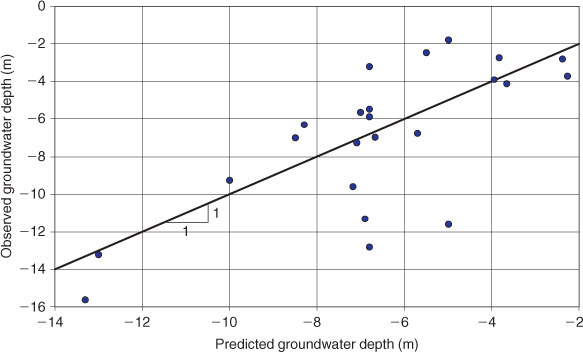
|

|
Predicting the base-flow index
The statistical model used to infer the base-flow contribution throughout the catchment had the form:

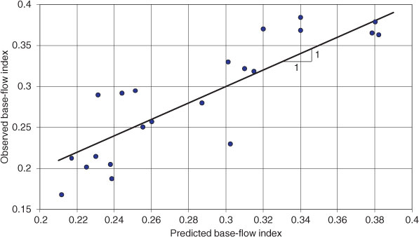
Of these potential predictors, we identified a reasonable (R 2 = 0.68) and highly significant relationship between BFI and rainfall (P < 0.001) and PET (P = 0.024).
The parameters c, d 1 and d 2 listed in Table 1 were estimated so that the best fit to the observed base-flow indices was obtained (Fig. 5). The observed and predicted levels of BFI for the 24 sites used in this analysis with a 1 : 1 line superimposed are shown in Fig. 5.
|
Identifying priority areas for rehabilitation
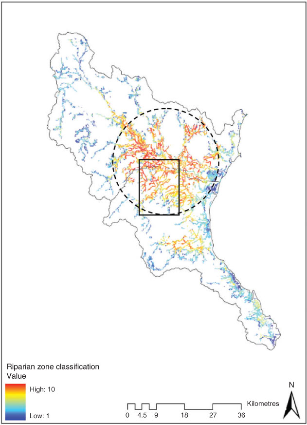
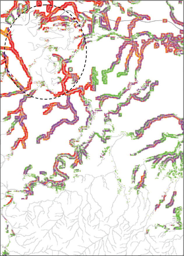
The modelling exercise suggested that riparian zone rehabilitation should first target streams in the central areas of the catchment (encircled area of Fig. 6). Lower-order streams found in the upper steeper parts of the Tully–Murray basin have a much lower rehabilitation potential and hence are low-priority areas for rehabilitation. Fig. 7 shows a more detailed view of the stream network that demonstrates the priority areas. Land use in this particular subregion in the catchment is agricultural and thus attained a high rehabilitation score. The encircled area had the highest score (~9) because it was the flattest within this subregion. Other areas (e.g. south and east of this region) had lower scores, ranging from 4 to 6.
|
|
Discussion
In the present study, we chose to simplify the complex processes that underpin denitrification and build a model based on our best conceptual understanding of the system. The adopted indices of the RMT have been validated by field measurements and have been shown to represent the underlying physical processes associated with nitrate generation and its potential removal via denitrification in riparian zones.
The particular strength of the RMT is the fact that it is a relative assessment tool that is used mainly to prioritise riparian rehabilitation on the basis of identifying the potential to generate nitrate and its removal via denitrification. Therefore, we are not attempting to provide an absolute estimate for denitrification potential, rather we are attempting to identify areas that are more likely to be conducive to denitrification based on our knowledge of landform and hydrology. The complex issue of evaluating river base flow is simplified by adopting a hierarchical system of base-flow indices that ranks the level of base-flow contribution to stream flow. Gu et al. (2008) concluded that during base-flow conditions, relatively deep groundwater flow paths carrying water containing high nitrate concentrations discharged through the streambed sediments, and high denitrification rates were observed along with a substantial reduction in the nitrate concentration. The highly variable contamination potential also uses a hierarchical system that eliminates the need to specify actual contaminant concentrations, but recognises various land uses as indicators for the level of contamination, with the highest contributor being agriculture. Hallberg (1989) reported that agriculture is the most extensive anthropogenic source of nitrogen to groundwater systems. The conceptual model for riparian hydrology uses the Darcy flux to calculate residence time; this flux accounts for the critical effect of depth to groundwater table, thus defining the denitrification potential in a spatially explicit manner.
The RMT adopts many simplifying assumptions regarding how it models nitrate removal in riparian zones. We recognise here some of the assumptions that may be violated in the natural environment. The model assumes that nitrate is removed as the groundwater flows through the carbon-rich root zone before it discharges to a stream. However, it is recognised that many streams have high NO3 concentrations in the base flow, which suggests that groundwater discharging to streams may be relatively unaffected by denitrification in the riparian soils (Böhlke et al. 2002). The configurations of aquifer redox zones near discharge areas are poorly known, but can have a major effect on the transfer of NO3 to surface waters (Böhlke et al. 2002). The RMT assumes that anoxic conditions prevail in the saturated root zone. Korom (1992) reported that the cut-off point where O2 concentrations are great enough for the cessation of denitrification varies greatly among organisms.
The RMT considers organic carbon to be the sole electron donor. Organic matter is the most abundant electron donor in the presence of a variety of electron acceptors in the saturated zone (Korom 1992). It is recognised that other electron donors exist; Böhlke et al. (2002) identified three different environments of denitrification within one transect where the reduction of O2 and NO3 was coupled with the oxidation of reduced Fe and S phases. In the absence of detailed knowledge regarding the variability of the denitrification potential on a catchment scale (which is most likely the case), assuming a constant maximum potential at the surface (R max) is appropriate. The RMT recognises a variable denitrification rate that declines with depth, thus aligning with organic carbon availability. Böhlke et al. (2002) stated that near-surface organic-rich sediments appear to have a relatively large potential supply of reactive electron donors (denitrification capacity); they added that NO3-rich groundwater can avoid these sediments by following a deeper flow path. Harms et al. (2009) conducted a two-site study and showed that the depth to the water table has a significant impact on the denitrification potential. Hence, the concept of relating the denitrification potential to the depth of the saturated root zone is sound.
There is a recognised lack of reliable information available to land managers to support their decision-making on nitrogen management issues that potentially compromises the effectiveness of their rehabilitation efforts. The spatial variability of the factors that control denitrification in riparian zones renders the task of identifying areas of optimal benefits a difficult one. In general, riparian rehabilitation should target low areas in the landscape (that have shallow water tables), flat areas (that allow a high residence time for denitrification to occur), regions of medium hydraulic conductivity soils (that allow a high flux and result in a relatively high water table), and areas where current land use results in high rates of nitrate delivery to streams. The focus for rehabilitation within these areas should then be on stream reaches where existing riparian buffers are in poor condition.
Dissolved inorganic nitrogen has been identified as the main pollutant in the Tully–Murray basin (Armour et al. 2009; Bainbridge et al. 2009). Implementation of the RMT in the Tully–Murray basin has identified areas where riparian rehabilitation is likely to yield optimal removal of nitrate through denitrification. This case study has shown that the RMT is a rapid assessment tool that can help land managers make science-based decisions on riparian management issues.
Acknowledgements
This work was funded by the Department of the Environment, Water, Heritage and the Arts. The development of the RMT was funded by the Cooperative Research Centre (CRC) for Catchment Hydrology and the CRC for Coastal Zone, Estuary and Waterway Management. The authors wish to thank research colleagues from the Queensland Department of Natural Resources and Water and Griffith University for their contributions. The constructive comments made by the reviewers, the journal editor and the guest editor have greatly improved the manuscript.
Armour, J. D. , Hateley, L. R. , and Pitt, G. L. (2009). Catchment modelling of sediment, nitrogen and phosphorus nutrient loads with SedNet/ANNEX in the Tully–Murray basin. Marine and Freshwater Research 60, 1091–1096.
Burford, J. R. , and Bremmer, J. M. (1975). Relationships between the denitrification capacities of soils and total, water-soluble and readily decomposable soil organic matter. Soil Biology & Biochemistry 7, 389–394.
| Crossref | GoogleScholarGoogle Scholar | CAS |
Cirmo, C. P. , and McDonnell, J. J. (1997). Linking the hydrologic and biogeochemical controls of nitrogen transport in near-stream zones of temperate-forested catchments: a review. Journal of Hydrology 199, 88–120.
| Crossref | GoogleScholarGoogle Scholar | CAS |
Devito, K. J. , Fitzgerald, D. , Hill, A. R. , and Aravena, R. (2000). Nitrate dynamics in relation to lithology and hydrologic flow path in a river riparian zone. Journal of Environmental Quality 29, 1075–1084.
| CAS |
Gallant, J. C. , and Dowling, T. I. (2003). A multi-resolution index of valley bottom flatness for mapping depositional areas. Water Resources Research 39, 1347–1360.
| Crossref | GoogleScholarGoogle Scholar |
Harms, T. K. , Wentz, E. A. , and Grimm, N. B. (2009). Spatial heterogeneity of denitrification in semi-arid floodplains. Ecosystems 12, 129–143.
| Crossref | GoogleScholarGoogle Scholar | CAS |
Inamdar, S. P. , Sheridan, J. M. , Williams, R. G. , Bosch, D. D. , and Lowrance, R. R. , et al. (1999a). Riparian Ecosystem Management Model (REMM): I. Testing of the hydrologic component for a coastal plain riparian system. Transactions of the American Society of Agricultural and Biological Engineers 42, 1679–1689.
Mazvimavi, D. , Meijerink, A. M. , and Stein, A. (2004). Prediction of base flows from basin characteristics: a case study from Zimbabwe. Hydrological Sciences Journal 49, 703–715.
| Crossref | GoogleScholarGoogle Scholar |
O’Callaghan, J. F. , and Mark, D. M. (1984). The extraction of drainage networks from digital elevation data. Computer Vision Graphics and Image Processing 28, 323–344.
| Crossref | GoogleScholarGoogle Scholar |
Rassam, D. W. , Fellows, C. , DeHayr, R. , Hunter, H. , and Bloesch, P. (2006). The hydrology of riparian buffer zones; two case studies in an ephemeral and a perennial stream. Journal of Hydrology 325, 308–324.
| Crossref | GoogleScholarGoogle Scholar |
Tucker, M. A. , Thomas, D. L. , Bosch, D. D. , and Vellidis, G. (2000a). GIS-based coupling of GLEAMS and REMM hydrology: I. Development and sensitivity. Transactions of the American Society of Agricultural and Biological Engineers 43, 1525–1534.

Tucker, M. A. , Thomas, D. L. , Bosch, D. D. , and Vellidis, G. (2000b). GIS-based coupling of GLEAMS and REMM hydrology: II. Field test results. Transactions of the American Society of Agricultural and Biological Engineers 43, 1535–1544.
van den Heuvel, R. N. , Hefting, M. M. , Tan, N. C. , Jetten, M. S. , and Verhoeven, J. T. (2009). N2O emission hotspots at different spatial scales and governing factors for small scale hotspots. Science of the Total Environment 407, 2325–2332.
| Crossref | GoogleScholarGoogle Scholar | PubMed | CAS |
Vidon, P. G. , and Hill, A. R. (2004). Landscape controls on the hydrology of stream riparian zones. Journal of Hydrology 292, 210–228.
| Crossref | GoogleScholarGoogle Scholar |