

Cost-effective water quality improvement in linked terrestrial and marine ecosystems: a spatial environmental–economic modelling approach
P. C. Roebeling A E , M. E. van Grieken B , A. J. Webster C , J. Biggs D and P. Thorburn DA CESAM – University of Aveiro, Department of Environment, 3810-193 Aveiro, Portugal.
B CSIRO Sustainable Ecosystems, Davies Laboratory, PMB PO, Aitkenvale, Qld 4814, Australia.
C CSIRO Sustainable Ecosystems, ATFI, PO Box 12139, Cairns, Qld 4870, Australia.
D CSIRO Sustainable Ecosystems, 306 Carmody Road, St Lucia, Qld 4067, Australia.
E Corresponding author. Email: peter.roebeling@ua.pt
Marine and Freshwater Research 60(11) 1150-1158 https://doi.org/10.1071/MF08346
Submitted: 16 December 2008 Accepted: 7 August 2009 Published: 17 November 2009
Abstract
Worldwide, coastal and marine ecosystems are affected by water pollution originating from coastal river catchments, even though ecosystems such as the Great Barrier Reef are vital from an environmental as well as an economic perspective. Improved management of coastal catchment resources is needed to remediate this serious and growing problem through, e.g. agricultural land use and management practice change. This may, however, be very costly and, consequently, there is a need to explore how water quality improvement can be achieved at least cost. In the present paper, we develop an environmental–economic modelling approach that integrates an agricultural production system simulation model and a catchment water quality model into a spatial environmental–economic land-use model to explore patterns of land use and management practice that most cost-effectively achieve specified water quality targets and, in turn, estimate corresponding water pollution abatement cost functions. In a case study of sediment and nutrient water pollution by the sugarcane and grazing industries in the Tully–Murray catchment (Queensland, Australia), it is shown that considerable improvements in water quality can be obtained at no additional cost, or even benefit, to the agricultural industry, whereas larger water quality improvements come at a significant cost to the agricultural industry.
Additional keywords: cost-effectiveness, diffuse source pollution.
Introduction
Worldwide, coastal and marine ecosystems are increasingly affected by point- and diffuse-source water pollution originating from rural, urban and industrial land uses in coastal river catchments (e.g. Gabric and Bell 1993; Furnas 2003; Fabricius 2005), even though ecosystems such as the Great Barrier Reef (GBR) are of vital importance from an environmental as well as an economic perspective (e.g. Cesar 2000; Elofsson et al. 2003; Productivity Commission 2003). For the GBR region in Australia, several studies have shown that agricultural development and altered land-use patterns in GBR catchments have led to increased rates of sediment and nutrient deliveries to the GBR lagoon (Gabric and Bell 1993; Neil et al. 2002; Furnas 2003). Improved management of coastal catchment land and water resources is needed to remediate this serious and growing problem through, e.g. agricultural land use and management practice change (Gabric and Bell 1993; Bramley and Roth 2002; Productivity Commission 2003). Changing land use and management practices may, however, be very costly and, consequently, there is a need to explore how water quality improvement targets can be achieved at least cost (Elofsson et al. 2003; Yang et al. 2005).
Several approaches combine land-use models with hydrological, ecological and/or soil models, in which environmental externalities from agricultural production impacting the downstream environment are analysed (for an overview, see Nelson 2002; Elofsson et al. 2003; Janssen and Van Ittersum 2007). Some studies have related land-use location and associated biophysical conditions to economic production potentials, but have either ignored or failed to spatially explicitly account for environmental impacts (see e.g. Johnsen 1993; Yiridoe and Weersink 1998; Rounsevell et al. 2003; Hajkowicz et al. 2005). Other studies have related land-use location and associated biophysical conditions to environmental impacts, but have either ignored or failed to spatially explicitly account for economic impacts (see e.g. Prosser et al. 2001; Neitsch et al. 2002; Lu et al. 2004). Few studies have integrated economic models with hydrological and/or soil models to explore opportunities for cost-effective water quality improvement through, e.g. targeting of conservation tillage, land retirement and riparian buffers at the catchment scale (see Khanna et al. 2003; Yang and Weersink 2004; Yang et al. 2005).
The present study contributes to previous research through the development of an interdisciplinary environmental–economic modelling approach that integrates an agricultural production system simulation model and a catchment water quality model into a spatial environmental–economic land-use model to explore patterns of land use and management practice that most cost-effectively achieve specified water quality targets and, in turn, estimate corresponding water pollution abatement cost functions. We develop and apply the Environmental Economic Spatial Investment Prioritisation (EESIP) modelling approach (Roebeling et al. 2006, 2007b) – an interdisciplinary environmental–economic approach to cost-effective water quality management in linked terrestrial and marine ecosystems. A case study is provided for total suspended sediment (TSS) and dissolved inorganic nitrogen (DIN) water pollution by the sugarcane and grazing industries in the Tully–Murray catchment (Queensland, Australia).
The EESIP modelling approach
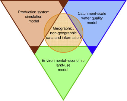
The EESIP modelling approach integrates three main components (Fig. 1; Roebeling et al. 2006, 2007b): (i) an agricultural production system simulation model, (ii) a catchment water quality model and (iii) a spatial environmental–economic land-use model. All models share a common database, containing geographically and non-geographically referenced data and information.
|
In brief, the agricultural production system simulation model assesses plot-level production and water pollution characteristics for a wide range of agricultural land use and management practices, the catchment water quality model assesses the relationship between local water pollution supply (i.e. gross supply of water pollutants to streams and rivers) and end-of-catchment water pollution delivery (i.e. net delivery of water pollutants to the coast), and, in turn, the spatial environmental–economic land-use model allocates agricultural land use and management practices such that they contribute most to regional agricultural income, given specified end-of-catchment water quality targets.
Production system simulation models
Agricultural land uses can be implemented using a wide variety of management practices, such as ways in which soils are prepared, crops are treated and cattle are managed. To assess the characteristics of agricultural land use and management practices with respect to their potential to contribute to local water pollution supply as well as their production potential and input requirements, we use two production system simulation models: the Agricultural Production Systems SIMulator (APSIM) for sugarcane production (Keating et al. 2003) and the Pasture and Animal System Technical coefficient generaTOR (PASTOR) for pasture-based beef production (Bouman et al. 1998).
The APSIM production system simulation model simulates, for a uniform block of cane, the per hectare long-term dry cane and sucrose weight, ground cover, soil water balance and nitrogen uptake and partitioning to leaf and cane stem. Model simulation results are determined by soil factors such as depth, water-holding capacity and nitrogen availability, management factors such as planting date, harvesting date, crop residue management and fertiliser use, genetic factors such as sugarcane variety, and climatic factors such as rainfall, radiation and temperature. For the Tully–Murray catchment case study, a middle-maturing cane variety is considered (Roebeling et al. 2007a). Assessed management practices include: (i) three tillage management practices (current, minimum and zero tillage), (ii) two fallow management practices (bare and legume fallow), (iii) six nitrogen application rates (from 60 to 210 kg ha–1 and nitrogen replacement), (iv) two nitrogen application methods (single and split application), (v) two herbicide application rates (current and reduced application), (vi) one headland type (grassed headlands) and (vii) one trash management practice (green cane trash blanketing). For further details on sugarcane production systems, see Keating et al. (2003), Thorburn et al. (2007) and Roebeling et al. (2007a).
The PASTOR production system simulation model simulates, for a uniform block of grazing land, the per hectare long-term beef production, ground cover and nutrient balances given the complex interaction between pasture growth and stocking rate. Consequently, PASTOR contains separate modules for the calculation of input–output figures for pasture, herd and feed supplement systems. Model simulation results are determined by soil factors such as drainage capacity and nitrogen availability, management factors such as stocking rate, fertiliser use and supplement provision, genetic factors such as pasture variety and cattle breed, and climatic factors like rainfall, radiation and temperature. For the Tully–Murray catchment case study, a signal grass (Brachiaria decumbens) fertilised pasture system and a Brahman-cross fattening system is considered (Teitzel 1992). Assessed management practices include: (i) 15 stocking rates (0.5 animal units per ha to 4.0 animal units per ha) and (ii) 11 nitrogen application rates (from 0 to 100% of the application rate that is required to obtain the maximum attainable yield). For further details on wet tropics grazing systems, see Teitzel (1992), Bouman et al. (1998) and Roebeling et al. (2007a).
APSIM and PASTOR thus generate plot-level (average annual) input–output data for all combinations of management practices, which, in combination with four soil classes (based on Murtha and Smith 1994) and one set of climate conditions (SILO 2006) for the Tully–Murray catchment, results in 576 and 660 unique combinations of inputs and corresponding outputs for sugarcane and pasture-based beef production, respectively (Roebeling et al. 2007a). Inputs include cattle, fertilisers, herbicides, labour and machinery, whereas outputs include sugarcane/beef production, C-factor values and DIN-concentrations. In turn, the Sediment River Network model/Annual Network Nutrient Export (SedNet/ANNEX) model uses these plot-level C-factor values and DIN-concentrations to estimate the location-specific per hectare contribution of these land use and management practices to end-of-catchment TSS and DIN delivery respectively (see below). TSS delivery estimates from land use and management practices are thereby based on the revised universal soil loss equation (RUSLE; Renard et al. 1997) in which the C-factor accounts for crop, cover and tillage method (Stone and Hilborn 2000), whereas DIN delivery estimates from land use and management practices are based on plot-level inorganic nitrogen concentrations (Wilkinson et al. 2004).
Catchment-scale water quality models
To assess the relationship between local water pollution supply and end-of-catchment water pollution delivery, we utilise the catchment water quality model SedNet/ANNEX. SedNet/ANNEX was originally developed as part of the National Land and Water Resources Audit (NLWRA) by CSIRO Land and Water (Prosser et al. 2001; DeRose et al. 2002). The SedNet/ANNEX model calculates the mean annual supply, within-catchment deposition and subsequent downstream delivery of sediments and nutrients through the construction of sediment and nutrient budgets for river networks.
A sediment/nutrient budget is an account of the most important sources and sinks for eroded material and physical nutrients (Wilkinson et al. 2004; Cogle et al. 2006). Sources of sediment include hillslope erosion, gully erosion, stream erosion, bank erosion and drain erosion; sinks for sediment include floodplain deposition, river bed deposition and reservoir deposition. Similarly, sources of nutrients include particulate nutrient erosion, dissolved nutrient run-off and point source nutrient pollution; sinks for nutrients are associated with sediment deposition, denitrification and phosphorus adsorption/desorption. Total sediment/nutrient delivery at the river mouth is the net result of the above processes in upstream internal watersheds and connecting gullies, streams and rivers.
To determine the relationship between local water pollution supply (from agricultural land use and management practices) and end-of-catchment water pollution delivery, the fraction χi of local water pollution supply ci from location i ending up at the river mouth is estimated. Hence, plot level C-factor values and DIN-concentrations for land use and management practices are estimated using crop growth simulation models (described earlier), and minimum and maximum plot level C-factor values and DIN-concentrations (as determined by the different management practices) are derived for each land use. SedNet/ANNEX simulations are subsequently performed for C-factor values and DIN-concentrations in between these minimum and maximum values to determine the local water pollution supplies ciTSS and ciDIN (in t) and corresponding end-of-catchment water pollution deliveries DiTSS and DiDIN (in t) for each location i. Equating these local water pollution supplies ci (in t) and corresponding end-of-catchment water pollution deliveries Di (in t) yields the fractions χiTSS and χiDIN of local water pollution supplies ci from location i ending up at the river mouth.
On the basis of plot-level C-factor values and DIN-concentrations of land use and management practices, we thus estimate for all locations i the per hectare contribution of these land use and management practices to end-of-catchment (mean annual) TSS and DIN delivery respectively. For the Tully–Murray case study, SedNet/ANNEX parameter values are taken from Armour et al. (2009).
Spatial environmental–economic land-use model
To explore agricultural land use and management practice patterns that most cost-effectively achieve water quality improvement targets and to estimate corresponding water pollution abatement cost functions, the EESIP modelling approach integrates results from the agricultural production system simulation model (APSIM/PASTOR) and the catchment water quality model (SedNet/ANNEX) into a spatial environmental–economic land-use model (Roebeling et al. 2006, 2007b).
The modelling approach recognises that (Roebeling et al. 2007b): (i) biophysical characteristics of the land vary according to location and, in turn, determine agricultural production potentials; (ii) climatic and geomorphologic conditions differ according to location and, in combination with land use and management practice, determine local water pollution supply and catchment water pollution delivery; and (iii) farmers use existing infrastructure to transport their produce to the processing plant or market. In addition, differences in fixed and variable costs and potential benefits from alternative agri-industrial processing options are considered.
Agricultural land use and management practices are allocated at the regional scale on the basis of which land use and management practice on a particular land unit contributes most to regional agricultural income, where regional agricultural income is defined as total production value (based on final products) less corresponding fixed and variable production, transport and processing costs. The mathematical optimisation model, which is solved using GAMS 2.50 – CONOPT 3 (Brooke et al. 1998), is structured as follows:
The total agricultural area a in the region is divided into uniform land-use blocks Li,j,k, where each block of land is: (i) geographically referenced by a site-specific identification tag (i), (ii) used to grow a specific crop (j) and (iii) using a particular management practice (k). Each land-use site Li,j,k is characterised by a distance to the processing plant or market by road di road or rail di rail (in km), specific soil characteristics and associated yields yi,j,k (in t ha–1), and specific production costs qi,j,k (in A$ ha–1) (see above). The region maximises regional agricultural income π, so that:
where pj is the price of final product j (market price in A$ t–1), hj is the fraction of final product per unit of crop, vroad and vrail are the variable transport costs by road and rail (in A$ t–1 km–1), vproc are the variable processing costs (in A$ t–1), and where frail and fproc are total fixed costs associated to rail and processing infrastructure (in A$). For each product j, the mode of transport is pre-defined to be either road (j = 1, …, n) or rail (j = n+1, …, N). The objective function is maximised subject to a block size and crop area constraint, which are respectively given by:
with ai the block size (in ha) and aj the maximum crop area (in ha).
End-of-catchment water pollution delivery Di (in t) from agricultural land use j and management practice k at location i is determined by the fraction χi of local water pollution supply ci,j,k (in t) ending up at the river mouth (see above), such that:
Catchment water pollution delivery D (in t) from all land uses and management practices in the catchment is given by the sum of water pollution deliveries Di for all locations i in the catchment. Eqn 4 is repeated for each water pollutant separately.
Application of the EESIP modelling approach to the Tully–Murray case study
Calibrated relative to QLUMP (2004) land-use data, a numerical application of the EESIP modelling approach is provided for TSS and DIN water pollution by the sugarcane and grazing industries in the Tully–Murray catchment, Queensland, Australia. EESIP uses constant 2005 input prices, average 2003–2005 output prices, detailed input–output figures (Roebeling et al. 2007b) as well as C-factor values and DIN-concentrations (based on Cogle et al. 2006; Armour et al. 2009) for management practices in sugarcane and grazing production (see previous section), in combination with spatially explicit information on elevation (QLUMP 2004) and soil class (based on Murtha and Smith 1994) as well as rail and road distance (Roebeling et al. 2006).
Baseline scenario
Baseline agricultural land use in the Tully–Murray catchment equals just over 72 000 ha, with sugarcane and grazing the dominant land uses covering ~50% and 30%, respectively of the total agricultural land use area (Table 1; Fig. 2) – other agricultural land uses include horticulture and forestry production (QLUMP 2004; Roebeling et al. 2007b). Water pollution delivery from sugarcane and grazing production in the Tully–Murray catchment equals ~42 kt TSS and 992 t DIN per year. For the same catchment, Armour et al. (2009) estimated annual water pollution delivery from sugarcane and grazing production at ~38 kt TSS and 932 t DIN, equivalent to over 30% of total TSS and 80% of total DIN delivery in the Tully–Murray catchment.

|

|
Small differences with Armour et al. (2009) are explained by the fact that their calculations are based on adapted QLUMP (2004) data, resulting in a much smaller grazing and a much larger forestry area than for the standard QLUMP (2004) land-use data that we used for our model calibration. In addition, our calculations are based on upper-bound DIN-concentration estimates for grazing systems (see Cogle et al. 2006) because we specifically deal with fertilised wet tropics grazing systems (see Teitzel 1992; Roebeling et al. 2007a). Finally, regional agricultural income from sugarcane and grazing production in the Tully–Murray catchment equals almost A$75 million per year – well in line with OESR (2004) estimates of almost A$150 million per year for the total agricultural production value in the Cardwell Shire.
Water quality target scenarios
In sugarcane production, reductions in TSS delivery of up to ~35% are expected to come at no additional cost to the industry – mainly through the adoption of soil-conservation practices (reduced and zero tillage) (Table 1; Fig. 2). Reductions in TSS delivery of over 35% would, however, come at a significant cost to the sugarcane industry and are most cost-effectively achieved through a reduction in the sugarcane area, altered fertiliser application rates and rearrangement of land management across the landscape. In particular, for ‘TSS –40%’ the most cost-effective fertiliser application rates are used on each soil type (150 kg N ha–1 on S1; 120 kg ha–1 on S2 and S4), whereas for ‘TSS –60%’ a significant amount of sugarcane land (on steepest slopes, on the least productive soil type S4 and furthest away from Tully) is taken out of production and fertiliser application rates on soil type S2 are increased to minimise subsequent foregone production returns.
In grazing production, reductions in TSS delivery are expected to come at a significant cost to the grazing industry as a result of a reduction in the grazing area in combination with the adoption of reduced stocking rates. Grazing land on the steepest slopes on the least productive soil type (S4) and furthest away from Tully is taken out of production first, whereas stocking rates (and subsequent nitrogen fertiliser application rates) are most cost-effectively reduced on the most productive soil type (S1) and furthest away from Tully.
Relative to DIN water pollution, in sugarcane production reductions in DIN delivery of up to ~50% are expected to come at no additional cost to the industry – mainly through the adoption of more nitrogen-efficient management practices (no over-application of fertilisers and split nitrogen application) (Table 2; Fig. 2). Reductions in DIN delivery of over 50% would, however, come at a significant cost to the sugarcane industry, and are most cost-effectively achieved through a further decrease in rates of nitrogen application, in particular on the least productive soil type (S4) and to a minor extent on the most productive soil types (S1 and S2) as the yield response to nitrogen application is largest on these most productive soil types.

|
In grazing production, reductions in DIN delivery are expected to come at a large cost to the grazing industry as a result of a reduction in the grazing area in combination with reduced rates of nitrogen application. Grazing land on the least productive soil type (S4) and furthest away from Tully is taken out of production first, while nitrogen application rates (and subsequent stocking rates) are most cost-effectively reduced on the most productive soil types (S1 and S2) furthest away from Tully.
Water pollution abatement cost functions
On the basis of the water quality target scenario results presented above, we estimated the water pollution abatement cost functions for each industry and each water pollutant by plotting the rate of water quality improvement (i.e. WQI = [D]Baseline – [D]Scenario) against the associated total water pollution abatement costs (i.e. WPAC = [π]Baseline – [π]Scenario) and fitting the quadratic water pollution abatement cost function:

where α1 and α2 are the linear and quadratic water pollution abatement cost coefficients, respectively. Corresponding parameter estimates (Table 3) are based on the presented water quality target scenarios and, consequently, water pollution abatement cost functions (Fig. 3) are given for values up to 60% (TSS) and 80% (DIN) of the industry’s potential to contribute to TSS and DIN water quality improvement, respectively.
|

|
In sugarcane production, considerable water quality improvements can be obtained at a negative cost (i.e. at a benefit to the sugarcane industry). Maximum benefits are expected to be obtained through a reduction in TSS and DIN water pollution of ~20% and 25%, respectively, and are facilitated through the adoption of win–win management practices (reduced tillage and zero tillage; economic optimum rates of fertiliser application, nitrogen replacement and split nitrogen application). While reductions in water pollution beyond these 20% (TSS) and 25% (DIN) come at a cost to the sugarcane industry, reductions in TSS and DIN delivery of up to 35% and 50%, respectively, are expected to come at no additional cost to the industry as compared with the current (baseline) situation. Yet, reductions in TSS and DIN delivery of over 35% and 50%, respectively, would come at a significant cost to the sugarcane industry – up to about A$8.1 million per year for a 60% decrease in TSS delivery and up to about A$6.2 million per year for an 80% decrease in DIN delivery.
In grazing production, all improvements in water quality come at a significant cost to the grazing industry (up to about A$2.5 million per year for a 60% decrease in TSS delivery and up to about A$5.6 million per year for an 80% decrease in DIN delivery), because of limited management practice options for water quality improvement.
Conclusions
Our results showed that considerable improvements in water quality can be obtained at no additional cost, or even benefit, to the agricultural industry, whereas larger water quality improvements come at a significant cost to the agricultural industry. However, there are large differences between industries. In sugarcane production, a 35% reduction in TSS delivery is expected to come at no additional cost (or even benefit) to the industry because of the adoption of reduced-tillage and zero-tillage practices, whereas a reduction in DIN delivery of up to 50% is expected to come at no additional cost (or even benefit) to the industry because of reduced over-application and split-application of fertilisers. A further reduction in TSS and DIN delivery would come at a significant cost to the industry as a result of a reduction in the sugarcane area and a further decrease in nitrogen application rates. In grazing production, reductions in TSS delivery are expected to come at a significant cost to the grazing industry as a result of a reduction in the grazing area in combination with the adoption of reduced stocking rates, while reductions in DIN delivery are expected to come at a large cost to the grazing industry as a result of a reduction in the grazing area in combination with reduced rates of nitrogen application. Finally, spatially explicit results indicated that TSS delivery is most cost-effectively reduced on paddocks that are located on the steepest slopes on the least productive soil types and furthest away from Tully, whereas DIN delivery is most cost-effectively reduced on paddocks that are located on the least productive soil types and furthest away from Tully.
The EESIP modelling approach presented in this paper contributes to previous approaches that integrate economic models with hydrological and/or soil models to explore opportunities for cost-effective water quality improvement (e.g. Khanna et al. 2003; Yang and Weersink 2004; Yang et al. 2005) because it integrates an agricultural production system simulation model as well as a catchment water quality model into a spatial environmental–economic land-use model – thus allowing for the simultaneous cost-effectiveness assessment of a wide variety of management practices for water quality improvement at the catchment scale. Hence, the EESIP modelling approach is used in the development of the Tully (Kroon 2008) and the Burdekin (ongoing) Water Quality Improvement Plans, in particular through the (spatially explicit) prioritisation of management practices that most cost-effectively contribute to water quality improvement.
Future research needs to address several limitations associated with the present study. First, industry water pollution abatement costs are based on the management practices assessed by Roebeling et al. (2007a) and, thus, do not include any alternative or future management practices for water quality improvement. It can be expected that industry water pollution abatement costs are lower if alternative or future management practices would also be taken into account, thus achieving larger water quality improvements at similar costs. To this end, industry alternative or future management practices for water quality improvement need to be identified, assessed and trialled, which requires research investments from the corresponding industry R&D organisations.
Second, and related to the previous point, industry water pollution abatement costs are based on current land-use patterns and, consequently, gains from land-use change between industries are not taken into account. It can be expected that aggregate agricultural water pollution abatement costs are lower if land-use change is taken into account, thus achieving larger water quality improvements at similar costs. This may, however, imply that some industries will partly disappear in favour of other (more cost-effective) industries.
Third, industry water pollution abatement costs are based on yield, input, labour and machinery costs associated with the adoption of considered management practices and, thus, do not include any other costs associated with the diffusion and adoption of management practices (see for example Vanclay and Lawrence 1995). In addition, TSS and DIN water pollution abatement costs functions are estimated separately, while, in most cases, sediment reduction measures also reduce nutrient emissions (and vice versa). For example, when we account for the DIN reduction impact of TSS reduction management practices, our results indicate that a 60% reduction in TSS delivery is accompanied by a 40% reduction in DIN delivery to the coast.
Fourth, the EESIP modelling approach is deterministic and thus likely to lead to biased outcomes. When the effectiveness of ‘best’ management practice adoption is uncertain while the cost of ‘best’ management practice adoption is (partially) irreversible, deterministic cost-effectiveness analyses result in biased outcomes as they do not take the quasi-option value of ‘best’ management practice adoption into account (Dixit and Pindyck 1994). Thomas et al. (2009) proposed the development of a Bayesian belief network for representing uncertainty relationships in GBR socio-ecological systems.
Finally, the EESIP modelling approach focuses on end-of-catchment water quality targets only and, thus, ignores freshwater quality standards and/or targets. Eutrophication of freshwater ecosystems in tropical Australia is, however, widespread (Brodie and Mitchell 2005) and potentially costly (Davis and Koop 2001). Consequently, freshwater quality should not be ignored when managing coastal catchment land and water resources to achieve water quality improvement in linked terrestrial and marine ecosystems.
Acknowledgements
The authors gratefully acknowledge the CSIRO Water for a Healthy Country Flagship, the Marine and Tropical Sciences Research Facility and the Terrain-NRM for facilitating this research. The authors thank Anne Henderson and Michael Hartcher (CSIRO) as well as John Armour and Louise Hateley (DNR&M) for their input and help in using SedNet/ANNEX. The authors also thank the anonymous referees for their helpful comments on earlier versions of this paper.
Armour, J. D. , Hateley, L. R. , and Pit, G. L. (2009). Catchment modelling of sediment, nitrogen and phosphorus nutrient loads with SedNet/ANNEX in the Tully–Murray basin. Marine and Freshwater Research 60, 1091–1096.
Bramley, R. G. V. , and Roth, C. H. (2002). Land-use effects on water quality in an intensively managed catchment in the Australian humid tropics. Marine and Freshwater Research 53, 931–940.
| Crossref | GoogleScholarGoogle Scholar | CAS |
Elofsson, K. , Gren, I. M. , and Folmer, H. (2003). Management of eutrophicated coastal ecosystems: a synopsis of the literature with emphasis on theory and methodology. Ecological Economics 47, 1–11.
| Crossref | GoogleScholarGoogle Scholar |
Gabric, A. J. , and Bell, P. R. F. (1993). Review of the effects of non-point nutrient loading on coastal ecosystems. Australian Journal of Marine and Freshwater Research 44, 261–283.
| Crossref | GoogleScholarGoogle Scholar | CAS |
Lu, H. , Moran, C. J. , Prosser, I. P. , and DeRose, R. (2004). Investment prioritization based on broadscale spatial budgeting to meet downstream targets for suspended sediment loads. Water Resources Research 40, 1–16.
| Crossref | GoogleScholarGoogle Scholar |
Neil, D. T. , Orpin, A. R. , Ridd, P. V. , and Yu, B. (2002). Sediment yield and impacts from river catchments to the Great Barrier Reef lagoon. Marine and Freshwater Research 53, 733–752.
| Crossref | GoogleScholarGoogle Scholar |
Nelson, G. C. (2002). Introduction to the special issue on spatial analysis for agricultural economists. Agricultural Economics 27, 197–200.
| Crossref | GoogleScholarGoogle Scholar |
Rounsevell, M. D. A. , Annetts, J. E. , Audsley, E. , Mayr, T. , and Reginster, I. (2003). Modelling the spatial distribution of agricultural land use at the regional scale. Agriculture Ecosystems and Environment 95, 465–479.
| Crossref | GoogleScholarGoogle Scholar |
Teitzel, J. K. (1992). Sustainable pasture systems in the humid tropics of Queensland. Tropical Grasslands 26, 196–205.
Thorburn, P. J. , Webster, A. J. , Biggs, I. M. , Biggs, J. S. , and Park, S. E. , et al. (2007). Towards innovative management of nitrogen fertilizer for a sustainable sugar industry. Proceedings of the Australian Society of Sugar Cane Technologists 25, 85–96.
Yang, W. , and Weersink, A. (2004). Cost-effective targeting of riparian buffers. Canadian Journal of Agricultural Economics 52, 17–34.
| Crossref | GoogleScholarGoogle Scholar |

Yang, W. , Sheng, C. , and Voroney, P. (2005). Spatial targeting of conservation tillage to improve water quality and carbon retention benefits. Canadian Journal of Agricultural Economics 53, 477–500.
| Crossref | GoogleScholarGoogle Scholar |
Yiridoe, E. K. , and Weersink, A. (1998). Marginal abatement costs of reducing groundwater N pollution with intensive and extensive farm management choices. Agricultural and Resource Economics Review 27, 169–185.