

Reef exposure to river-borne contaminants: a spatial model
M. Maughan A B C and J. Brodie BA Department of Environment and Resource Management, Northern Region, PO Box 5391, Townsville, Qld 4810, Australia.
B Australian Centre for Tropical Freshwater Research, James Cook University, Townsville, Qld 4811, Australia.
C Corresponding author. Email: mirjam.maughan@derm.qld.gov.au
Marine and Freshwater Research 60(11) 1132-1140 https://doi.org/10.1071/MF08328
Submitted: 1 December 2008 Accepted: 12 August 2009 Published: 17 November 2009
Abstract
Rivers flowing into the Great Barrier Reef carry contaminants such as suspended sediments, dissolved inorganic nitrogen, total phosphorus and pesticides. To measure the extent and direction of the contaminants after they enter the Great Barrier Reef lagoon, a model was created using river volume, flooding variability, contaminant load, distance and direction as inputs. A GIS was used to calculate and visualise the exposure of the contaminants to the reefs for the current day, as well as modelling scenarios for pre-European arrival loads, and land management using realistic targets set by a regional Natural Resource Management board for water quality improvement planning purposes. The results show that a reduction in the dissolved inorganic nitrogen load exiting the Tully and Murray Rivers reduces the exposure of reefs close to the basin, but that reefs further east of the basin are significantly influenced by other rivers, highlighting that management for water quality improvement in neighbouring basins is also required.
Additional keywords: dissolved inorganic nitrogen, GIS, herbicides, suspended sediments, total phosphorus.
Introduction
The Great Barrier Reef (GBR) is a reef system extending more than 2300 km along the north-eastern Australian coast (EPA 2003). Over 50 rivers flow into the GBR lagoon from the adjacent GBR catchment area (Geoscience Australia 2006). As land-based pollution is an important reason for the worldwide decline of reefs (Pandolfi et al. 2003), it is important to investigate the extent and influence of individual rivers and their contaminants, as well as the impact of the combination of these rivers.
Agricultural development of the GBR coast in the past 150 years has increased the run-off of sediments, nutrients (nitrogen and phosphorus) and herbicides to the reef (Brodie et al. 2008). Major industries in the region, such as beef grazing, have caused an increase in soil erosion and 4–5-fold the amount of sediment is now delivered to the reef compared with pre-European settlement. The use of fertiliser associated with cropping industries, such as sugarcane, horticulture and cotton, has increased the nutrient level in waters of the coastal area, and the herbicides and pesticides used in these industries were non-existent before European settlement. Urban centres along the GBR coast also contribute to increased nutrient levels (Brodie et al. 2003). These materials are having an impact on mangroves (Duke et al. 2005) and coral reefs (Fabricius et al. 2005) and causing reduced health, dieback and reduced richness and abundance of mangrove and coral species.
The level of exposure of the GBR lagoon to contaminants needs to be identified to manage the detrimental effects associated with these increased contaminants. This is a complex task because of a combination of multiple sources, ocean currents, wind directions, dilution, sediment settling and the natural break down of the contaminants. In the present study, we provide an improved version of our reef exposure model (Devlin et al. 2003).
Of all the pollutants generated on the GBR catchment and discharged into the GBR lagoon, total suspended sediments (TSS), dissolved inorganic nitrogen (DIN), total phosphorus (TP) and ‘Diuron’ type herbicides have been prioritised as presenting the greatest risk (Brodie et al. 2008). This simple model attempted to visualise the exposure of reefs to TSS, DIN, TP and herbicides. The model takes into account the river volume, variability of river floods flushing out to the ocean, distance from the river mouth, wind and current directions, and contaminant dispersal. Improvements to our previous version include: (i) increased number of reef data points (4200 v. 30); and (ii) ability to model the exposure by each contaminant individually, making it easier to visualise the influence of a single contaminant. The results of this modelling exercise have assisted the development of regional Water Quality Improvement Plans (WQIPs) in the GBR region.
Materials and methods
Study site
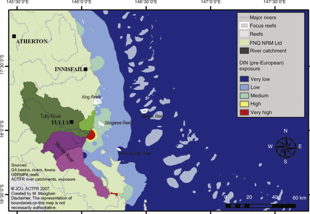
The focus area was the coastal waters off the Tully catchment (Fig. 1; Kroon 2009), although the model takes into account all rivers flowing into the GBR. Currents and wind transport contaminants along the coast and the reefs off Tully have an accumulated exposure originating from multiple rivers.
|
Data inputs
The data used to model the exposure include river exits from the 51 most important rivers flowing into the GBR, from the Burnett River in the south to the Jackey Jacky Creek in the north (Geoscience Australia 2006). To be able to measure the distance between river exit and reef, centroids were created for the 3000 reefs mapped by the Great Barrier Reef Marine Park Authority (GBRMPA 2003) and more points were added to create a continuous surface that could later be used for interpolation. The annual contaminant load for each of the rivers was taken from Brodie et al. (2003), which was the most complete data set for this study area for TSS, DIN and TP annual loads. The present study also summarises previously modelled estimates for pre-European arrival annual loads for TSS, DIN and TP using monitoring data from relatively untouched catchments in a similar climate. Monitored pesticide data were only available for three rivers (White et al. 2002; Mitchell et al. 2005; Lewis et al. 2007), so the annual pesticide load at the river mouth was predicted for the remaining rivers by comparing the area of pesticide-using-land-use of those three rivers to the area of pesticide-using-land-use in the remaining rivers, using Queensland Land Use Mapping Program (QLUMP) land-use data (Queensland Department of Natural Resources and Water 2002).
River volume data were taken from Furnas (2003), but because the numbers represented the whole basin they were transformed to represent the river only, after creating river catchments for each basin. There is a considerable difference in flow variability between the GBR rivers considered in the present analysis. We believe that rivers with low flow variability and hence frequent high-flow events, such as the Tully with multiple high flow events per year, present more of a risk to reef ecosystems than high variability rivers with very infrequent high-flow events, such as the Fitzroy River with high flow events only every few years. Part of the rationale behind this belief is that ecosystems of high variability rivers have extended recovery times, whereas ecosystems of low variability rivers never have long recovery times. Thus, a river flow variability factor was incorporated into the model. The variability for each river was taken from the Watershed database (Queensland Department of Natural Resources and Water 2006). To reflect the negative influence of more frequent floods on reef exposure, the inverse of variability was taken: 1/var. To compress the results and to limit the large influence of a few highly variable rivers (e.g. the Tully River with 1/var = 4.5), the square root was taken: √(1/var).
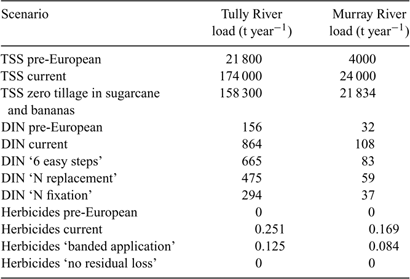
Aside from current and pre-European scenarios, management scenarios were set up with estimated results after recommended changes in land management for water quality improvement. In the Tully basin, the recommended changes in land management for water quality improvement included: (i) reduction in the DIN load after ‘six easy steps management’: using regular soil testing and adopting soil-specific nutrient management (BSES 2008), (ii) reduction in the DIN load after ‘nitrogen fixation’: growing special varieties of sugarcane that act to encourage the growth of (atmospheric) nitrogen-fixing bacteria to reduce the amount of applied fertiliser (Terrain 2009); and (iii) reduction in the herbicide load to no residual herbicide loss for both the Tully and Murray Rivers (Table 1). Modelling the influence of management regimes within the Tully catchment requires the removal of data from outside the Tully region to visualise the influence of one region’s management; thus, scenarios with and without the influence of other rivers were modelled.
|
Analysis
The distance between each river exit and reef centroid was calculated using the Point Distance tool in ArcGIS9.2 in a GDA 1994 MGA projection of zones 54, 55 and 56; limiting the calculation to a 500-km radius. The result was a table with nearly 100 000 unique ‘river-to-reef’ records, with each record displaying the source coordinates (river), destination coordinates (reef) and the distance between the two.
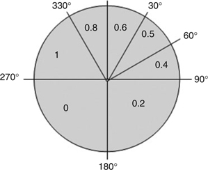
The bearing between each river exit and reef centroid was calculated using the coordinates (script by Snyder 2004); north was equal to 0°. We visualised the preferential direction of the river loads exiting into the GBR (Fig. 1); 1 was the prevalent flow direction and 0 was an unlikely flow direction. This visualisation was created with data from modelled and monitored flood plume studies in the GBR (King et al. 2001; Devlin and Brodie 2005); the north-western movement caused by the Coriolis effect (Rohde et al. 2006); prevailing south-easterly winds in the summer months (Devlin et al. 2001); the northward-flowing Hiri current (Brinkman et al. 2002) and the southward-flowing East Australian Current (Brinkman et al. 2002).
River-borne contaminants, such as TSS and DIN, behave quite differently after entering the GBR lagoon. The contaminants analysed in the present model can be divided into two groups: contaminants of a particulate nature that are affected by sedimentation processes (TSS and TP) and contaminants of a dissolved nature that are not affected by sedimentation (DIN and herbicides). The TSS sediments out rapidly near the river mouth (Devlin and Brodie 2005); hence, a dispersion factor proportioned to the square of the distance can be used to approximate the change of concentration in TSS and TP from the river mouth. In contrast, DIN mixes conservatively after discharge into the GBR lagoon (Devlin and Brodie 2005) and is not affected by sedimentation; thus, a dispersion factor proportioned to the distance can be used to approximate the change in the concentration of DIN and herbicides.
This river–reef combination table was then joined to a table with values from each river exit, including variability, discharge and contaminant concentration. Reef exposure could now be calculated using one of the following formulae:
DIN and herbicides:
-
Variability × discharge × contaminant concentration × bearing × 1/distance,
and TSS and TP:
-
Variability × discharge × contaminant concentration × bearing × 1/distance2.
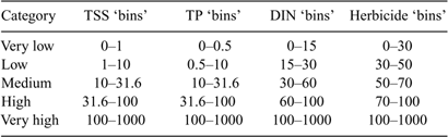
To visualise the results on a map, the exposure values of each reef were summarised in a pivot table: adding the exposure values of all rivers to that particular reef. These values were added to the reef layer in GIS and an inverse distance-weighted interpolation was used to create a continuous surface between each of the reef points of relative reef exposure. The values were visualised in five classes, ranging from very low to very high (Table 2), using expert knowledge and colour changes in flood plume satellite imagery (Fig. 2) to determine the values of each of the classes.
|

|
The results can be analysed from a reef perspective, that is, ‘what rivers impact this reef?’, as well as from a river perspective, that is, ‘how far does the influence of this river reach?’. Scenarios for both pre-European arrival (natural exposure) and current exposure were modelled using monitored and modelled input data, and management scenarios were modelled using achievable management strategies with the predicted reduction in contaminant load. Certain scenarios incorporated the influence from all GBR rivers, other scenarios focussed on the influence of the rivers of one region only, and a third group of scenarios looked at the result of management in one region while the other rivers maintained the same contaminant load.
Results and discussion
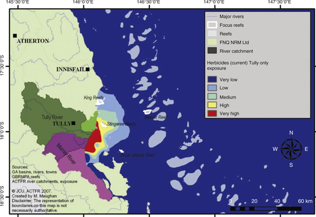
The pre-European scenario of DIN exposure in Tully under the ‘all river influence’ scenario (Fig. 3) shows that the coastal waters had medium to very high exposure, with Stingaree Reefs showing medium exposure. The current scenario (Fig. 4) reveals that the extent of DIN exposure has expanded; although for the pre-European scenario the medium exposure reefs were close to shore, the current scenario shows medium exposure further east, including the outer reefs. Stingaree and Bedarra Reefs show high exposure to DIN, but because of the naturally high exposure level in the coastal areas, the increase in exposure gives a clearer picture of the degree of changed exposure; Stingaree Reefs DIN exposure increased by 282% when the pre-European arrival and current scenarios were compared. The Tully River is responsible for 62% of Stingaree Reefs’ exposure, with other rivers such as the Herbert, Burdekin and Johnstone Rivers also influencing the water quality of this reef (Table 3).
|

|
|
The TSS exposure under an ‘all river influence’ scenario shows low exposure in the Tully region, reaching 20–30 km offshore, with medium to very high exposure close to the river mouths. When modelling the influence of the Tully–Murray Rivers only (Fig. 5), the TSS exposure on King and Brook Island Reefs is reduced to very low, from a low value in the all river scenario, indicating that these reefs are also influenced by rivers outside the Tully area. The data confirm that 52% of King Reefs’ exposure comes from Maria Creek and 55% of Brook Islands Reef’s exposure can be traced to the Herbert River, highlighting that improving reef health is a combined effort between regions.

|
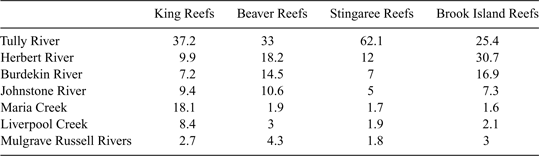
The source of herbicides for the Tully region reefs is also partially sourced outside the region, with King Reefs having a very high exposure under the ‘all river influence’ scenario and low exposure under the ‘Tully–Murray River influence’ scenario (Fig. 6). For the King, Beaver and Brook Island Reefs, the Tully River is the source of 16–25% of their herbicide exposure, with Maria Creek and Herbert River contributing another 15–27%.
|
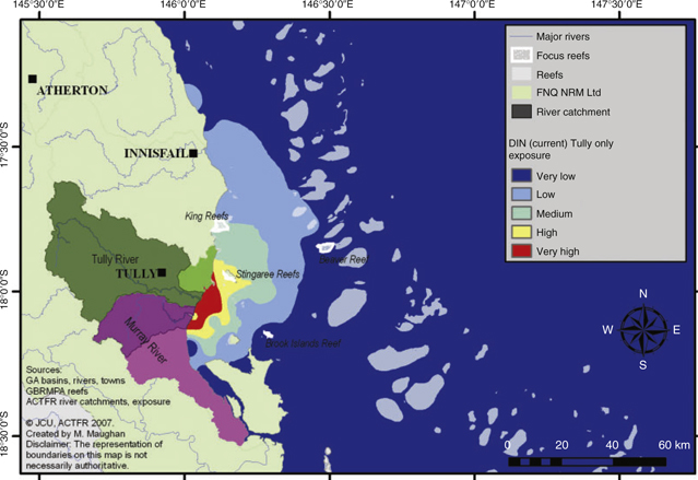
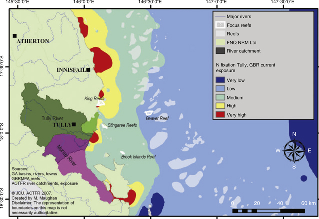
Without management, the medium DIN exposure just reaches the outer reefs in the east and the King Reefs north of the Tully River mouth (Fig. 7). When modelling the expected results from the DIN ‘N fixation’ management (Fig. 8), the exposure of King Reefs is reduced from medium to very low and the exposure of Stingaree Reefs is reduced from high to low, both with a reduction of 66%. When adding the current DIN levels of the other rivers to the picture (Fig. 9), the reduction of exposure for King Reefs is only 26% and the reduction for Stingaree Reefs is 43%: the Tully River is only responsible for 37% of King Reefs’ total exposure, with Maria Creek contributing 18%. The Tully River also affects reefs in other regions; although grouped in the ‘very low exposure’ class in the map, the Tully River is still the source of 6% of the DIN exposure of Geoffrey Bay Reef (Magnetic Island, east of Townsville) (Maughan et al. 2007).
|
|
|
When taking the influence of other rivers into account and reducing the herbicide residue in the run-off water to nil in the Tully region, the herbicide exposure of King Reefs is reduced by 34.9%, but is still influenced by Maria Creek. Stingaree Reefs has a 60% drop in the exposure, changing from very high to low exposure.
According to this model, the Tully River has one of the largest DIN extents of exposure of the GBR rivers, with the Whitsunday Islands receiving 1–2% of their DIN exposure from the Tully River (Maughan et al. 2007). This could be because the Tully River has the largest flooding variability (several floods per year), combined with high river volume and DIN loads. However, it must be noted that exposure in this model is a unit-less number and represents relative exposure. This model should be used to compare the influence of one river to another, or to visualise the reduction in exposure when managing the contaminant load in rivers. Different management scenarios can be compared to see which one has the desired outcome.
The model succeeded in improving the detail of previous models and can now calculate exposure to 4000 points, an increase from the 30 reefs modelled in Devlin et al. (2001). The reason why the present study modelled individual contaminants and not a combined exposure, as shown in Devlin et al. (2001), was to visualise each contaminant. In addition, adding contaminants raises the question of how different contaminants influence marine organisms. Octocorals have a stronger response to water quality change than hard corals (Fabricius et al. 2005), whereas seagrass decline is most commonly caused by a reduction in light from algal blooms after increases in nutrients (Schaffelke et al. 2005). Certain organisms might be affected more by a rise in DIN than a rise in TSS, and some species are more tolerant to water quality changes than others. A risk assessment was not the scope of this research, but could be added in the future.
Other future developments and improvements could include better input data for pesticides, a sensitivity analysis of each of the data inputs and a comparison of the results to chlorophyll and sediment data derived from satellite imagery.
Acknowledgements
Thanks go to Terrain NRM, Black Ross Basin WQIP, Burdekin Dry Tropics NRM, Mackay Whitsunday NRM Group, Burnet Mary NRM and the Fitzroy Basin Association for the research funding. Thanks also go to Will Higham for organising this project and to the Reef Partnership for facilitating the project.
Brinkman, R. , Wolanski, E. , Deleersnijder, E. , McAllister, F. , and Skirving, W. (2002). Oceanic inflow from the Coral Sea into the Great Barrier Reef. Estuarine, Coastal and Shelf Science 54, 655–668.
| Crossref | GoogleScholarGoogle Scholar |
Devlin, M. , and Brodie, J. (2005). Terrestrial discharge into the Great Barrier Reef Lagoon: nutrient behavior in coastal waters. Marine Pollution Bulletin 51, 9–22.
| Crossref | GoogleScholarGoogle Scholar | CAS | PubMed |
Duke, N. C. , Bell, A. M. , Pederson, D. K. , Roelfsema, C. M. , and Bengtson Nash, S. (2005). Herbicides implicated as the cause of severe mangrove dieback in the Mackay region, NE Australia: consequences for marine plant habitats of the GBR World Heritage Area. Marine Pollution Bulletin 51, 308–324.
| Crossref | GoogleScholarGoogle Scholar | CAS | PubMed |
Fabricius, K. , De’ath, G. , McCook, L. , Turak, E. , and Williams, D. (2005). Changes in algal, coral and fish assemblages along water quality gradients on the inshore Great Barrier Reef. Marine Pollution Bulletin 51, 384–398.
| Crossref | GoogleScholarGoogle Scholar | CAS | PubMed |
Kroon, F. (2009). Integrated research to improve water quality in the Great Barrier Reef region. Marine and Freshwater Research 60, i–iii.
Mitchell, C. , Brodie, J. , and White, I. (2005). Sediments, nutrients and pesticide residues in event flow conditions in streams of the Mackay Whitsunday Region, Australia. Marine Pollution Bulletin 51, 23–36.
| Crossref | GoogleScholarGoogle Scholar | CAS | PubMed |
Schaffelke, B. , Mellors, J. , and Duke, N. C. (2005). Water quality in the Great Barrier Reef region: responses of mangrove, seagrass and macroalgal communities. Marine Pollution Bulletin 51, 279–296.
| Crossref | GoogleScholarGoogle Scholar | CAS | PubMed |